Design of Power Cable Lines Partially Exposed to Direct Solar Radiation—Special Aspects

Abstract

Power cable lines are usually buried in the ground. However, in some cases, their ending sections are mounted along the supports of overhead lines. This leads to a situation where the cables are exposed to direct solar radiation and, consequentially, overheat. The paper presents the advanced computer modelling of power cables’ heating, considering their insolation as well as the effect of wind. The temperature and current-carrying capacity of power cables—during exposure to direct solar radiation—are evaluated. An effective method of limiting the unfavourable impact of the sun is discussed. In the presence of solar radiation, the proposed method enables a significant increase in the power cables current-carrying capacity.

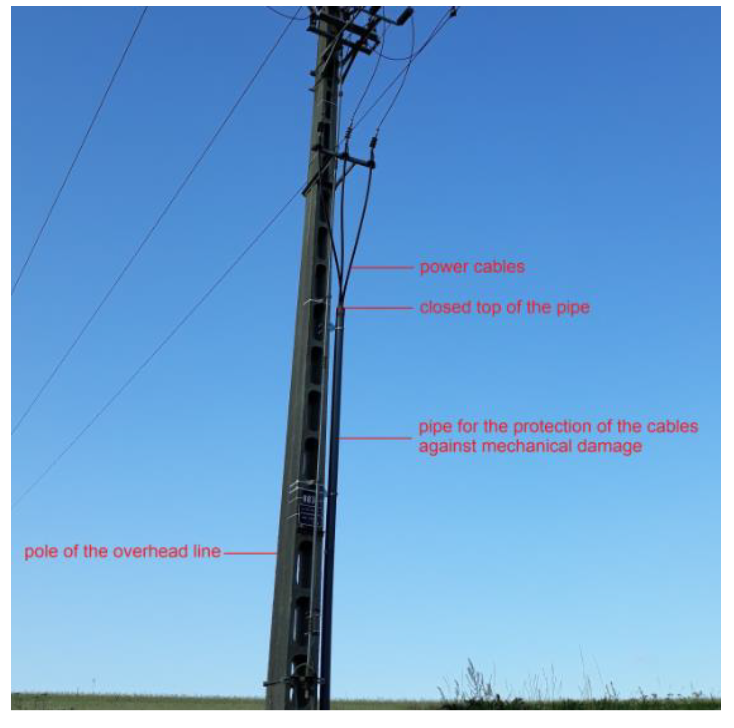
1. Introduction

One of the most important parameters of power cable lines is their current-carrying capacity. The rated load of the power cable line, in given external conditions, should not result in the temperature of cables (cables insulation) being higher than the maximum permissible temperature specified in the standard. However, in practice, there are cases of the thermal damage of power lines as a result of the overheating of the cables’ insulation, which reduces the thermal endurance of power cables, as well as the safety and reliability of power delivery [1,2,3,4,5]. The risk of power cables overheating results from the occurrence of adverse weather conditions (strong sunlight, no wind), which are sometimes overlooked by power network designers.

The basis of the designers’ work is their experience and the provision of dedicated standards. The main international standards [6,7,8,9,10] for determining the current-carrying capacity of power cables are based on the Neher–McGrath analytical calculation method published in 1957 [11,12,13]. A large number of scientists recognizes that the data contained in the indicated standards do not relate to the actual conditions of power line operation. Therefore, the current-carrying capacity values determined on the basis of these standards are divergent in comparison with the current-carrying capacity based on the experience and numerical calculations [3,14,15,16,17,18]. This is especially important in the case of the complicated layouts of cable systems or in the presence of unfavourable environmental conditions.

The paper [13] presents the influence of many factors on the current-carrying capacity of power cables in the air, among others the influence of wind speed, but without taking into account its direction in relation to the power cable axis. The paper contains an analysis of the impact of solar radiation on the permissible load but without an exact description of the radiation model. This paper also presents the impact of cables ventilation on their current-carrying capacity. However, the conditions of this process have not been clearly defined.

The authors of papers [19,20] analyzed the impact of wind direction and its speed on the current-carrying capacity of conductors. This analysis applied to one bare conductor of the overhead line. In turn, the author of the paper [21] presents an analysis of the current-carrying capacity of an overhead line in terms of the impact of wind speed and solar radiation based on analytical formulas, but does not take into account the impact of wind direction on the current-carrying capacity.

Increasing the current-carrying capacity of electrical devices as well as power cables is the subject of many scientists’ research [22,23,24,25,26,27]. It can be seen that the basis of these considerations is mainly the analysis of the thermodynamic state of power cables. In such cases, the geometry of the system and initial conditions are important, and the flow around cables is characterized by numbers: Nusselt Nu, Grashof Gr, Prandtl Pr. Calculations of these states can be carried out analytically or numerically.

In this paper, the results of the comprehensive ANSYS software-based numerical simulations of the thermal phenomena occurring in cables located in free air—during windy and/or sunny weather—are presented. Although some results of calculations of the current-carrying capacity for cables placed in free air are presented in the literature, the aforementioned ANSYS-based research, with the use of the authors’ heat transfer model of the PVC-insulated cable, enables modelling more complicated cases of ambient conditions as well as giving more precise results. The special aspect of the power cable line current-carrying capacity evaluation is also discussed—it refers to the power cable line changing the layout from the buried in the ground to the located in free air. The method for improving the thermal condition of such a cable line, based on passive cooling, utilizing natural/free convection and the buoyancy effect, is proposed. According to the proposed solution, power cables are placed in vertical pipe-channels, which intensify the thermal convection from the external surface of the cables. The optimization of the dimensions of the channel enables a significant increase in the current-carrying capacity of the cables. The authors’ proposal is economically attractive because it does not require an additional power supply and, hence, does not consume energy for the intensification of the favourable airflow along the channels.

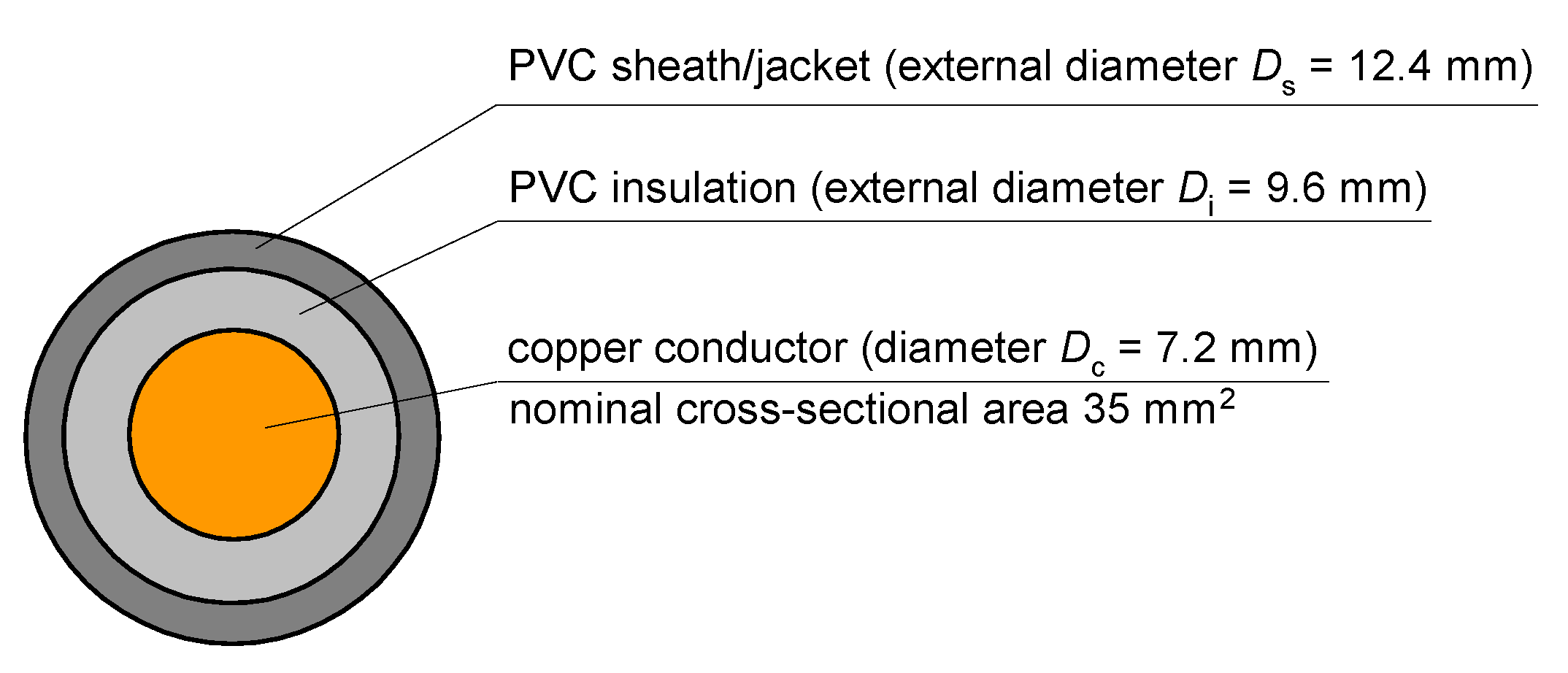
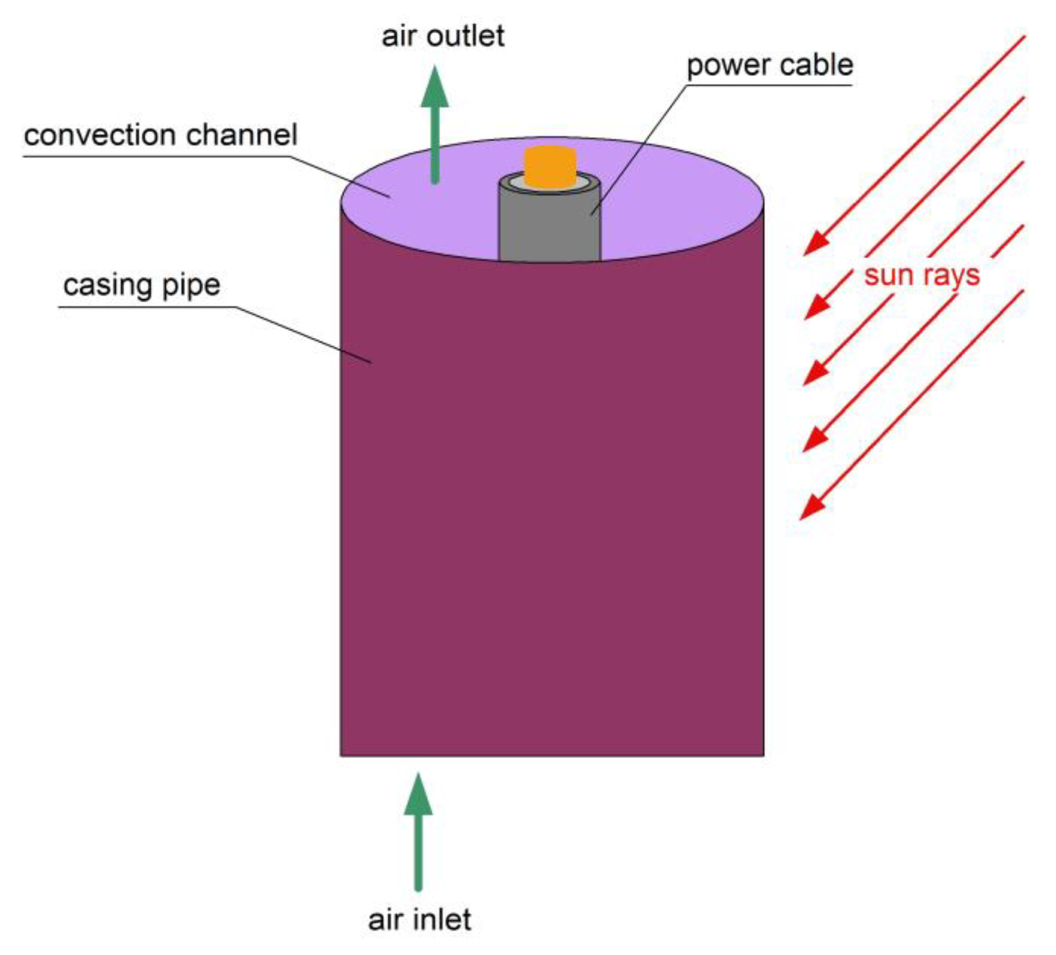
2. Description of the Numerical Model of the Cables

This article considers power cables composed of PVC insulation (permissible continuous temperature 70 °C), PVC sheath/jacket, and the multi-wire (stranded) copper conductor of nominal cross-sectional area equal to 35 mm². The construction of the power cable is shown in Figure 1.

By heat balance, heat is generated in the cables via the two following ways:

(1)

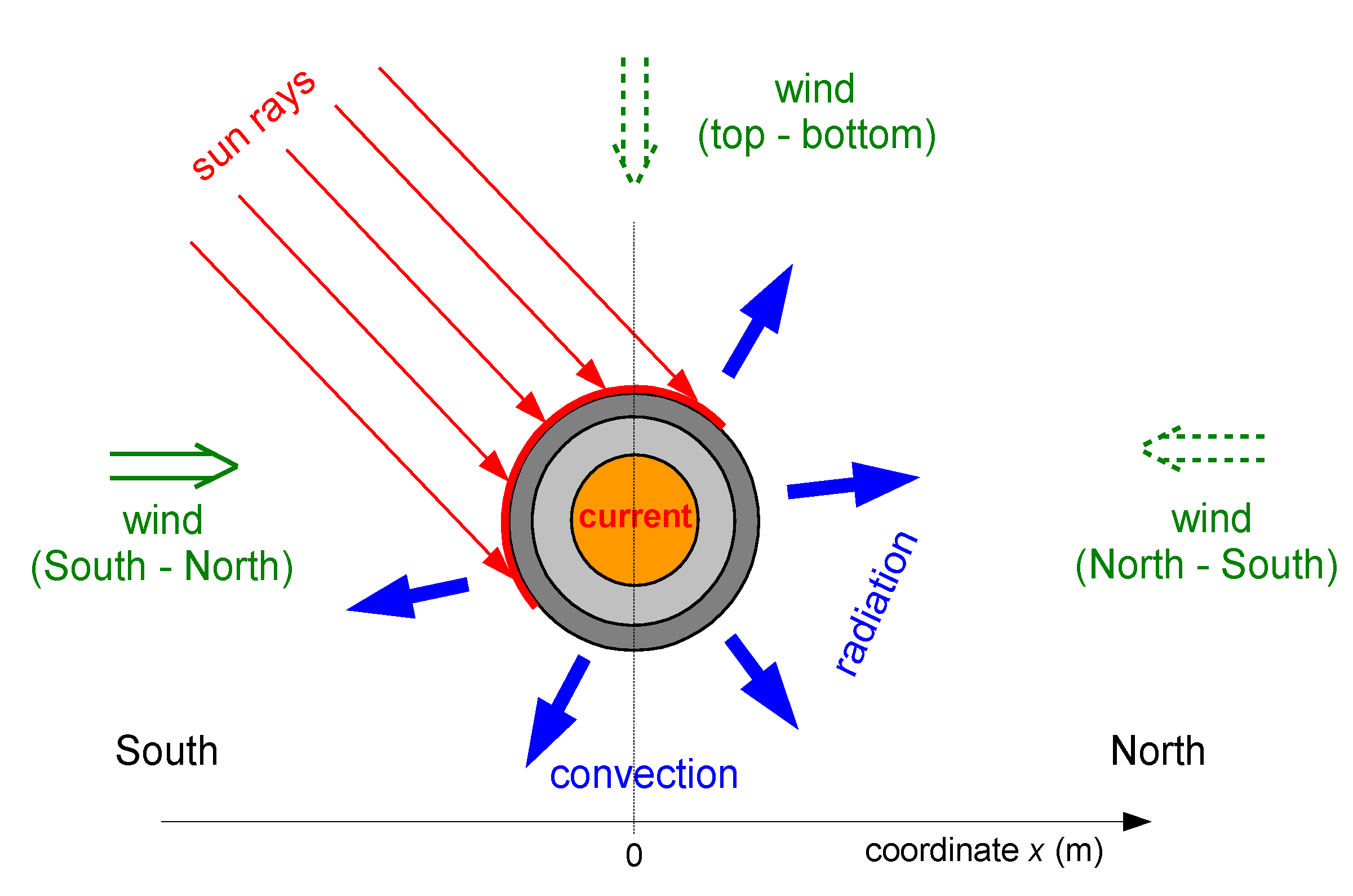
Joule’s heat produced by the current I_cc flowing through the copper conductor—in most of the studied cases, the boundary condition of Joule’s heat flux density q_Joule is iteratively introduced to obtain a result for which the max permissible temperature in any area of insulation is reached (70 °C). The current-carrying capacity I_cc is included in the following formula:

$$q_{\mathrm{Joule}}=\frac{q_{\mathrm{cc}}}{A_{\mathrm{c}}}=\frac{{I_{\mathrm{cc}}}^2\cdot R_{\mathrm{AC}}}{\pi \cdot D_{\mathrm{c}}\cdot L_{\mathrm{u}}} \Rightarrow I_{\mathrm{cc}}=\sqrt{\frac{q_{\mathrm{Joule}}\cdot \pi \cdot D_{\mathrm{c}}\cdot L_{\mathrm{u}}}{R_{\mathrm{AC}}}}$$

(1)

where:

• q_cc is the thermal power (heat) generated by the current in the power cable given length, W;
• A_c is the external/side surface of the copper conductor (dissipating heat to the ambient air), m²;
• I_cc is the current-carrying capacity, A;
• R_AC is the resistance of the power cable for AC current, Ω;
• D_c is the diameter of the copper conductor, m;
• L_u is the unit length of the copper conductor, m.

The heat flux density is equal to the ratio of thermal power q_cc separated on the unit length (usually 1 m) of the cable to the side surface of the copper conductor A_c with the unit length. The assumption made in the research is an even distribution of Joule’s heat flux density over the entire lateral surface of the copper conductor.

(2)

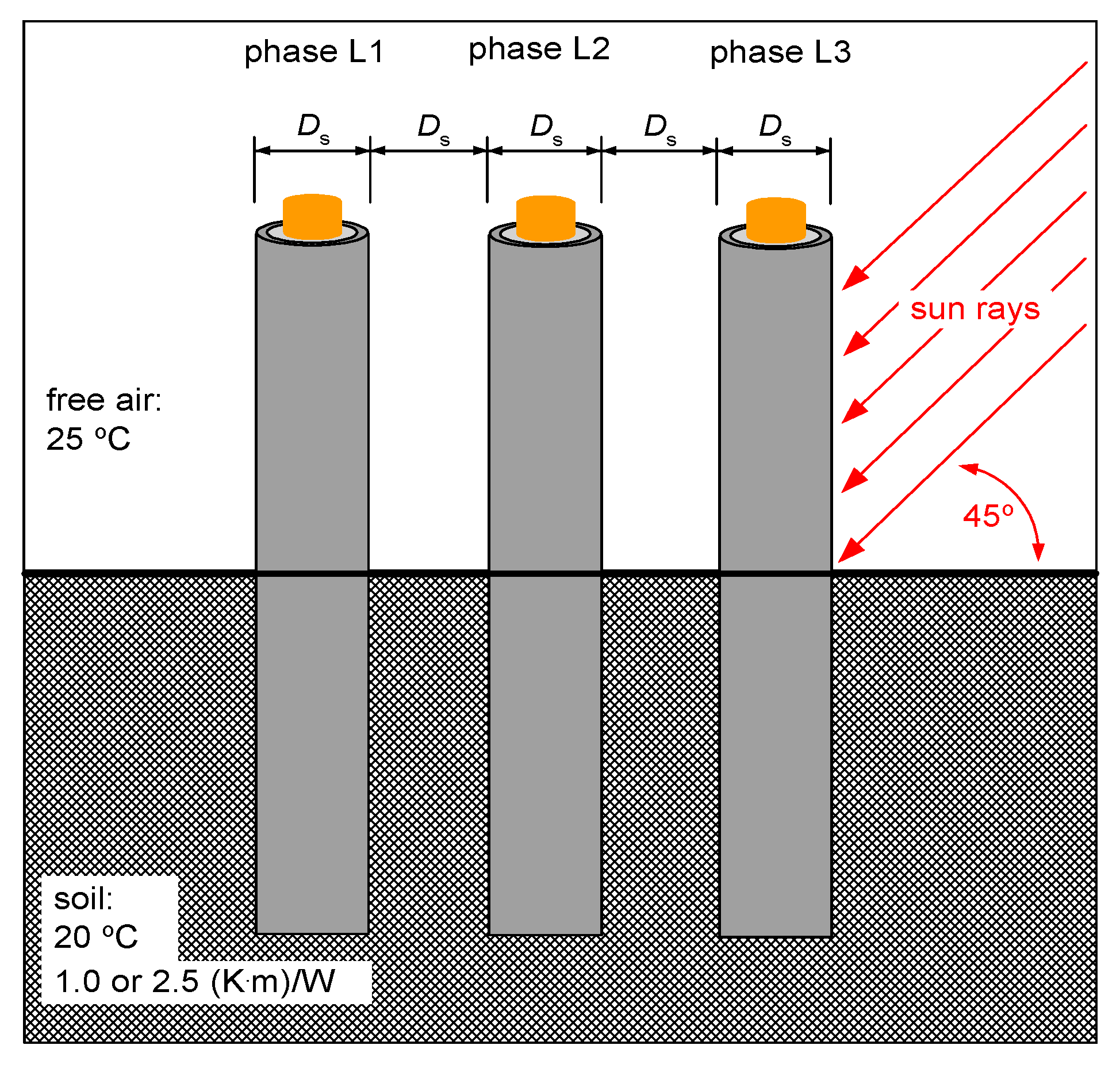
The heat generated by solar radiation—presented as the authors’ functional determination of the density of heat flux reaching the insulation surface q_solar(x), W/m². This relationship has been transformed for use in the Cartesian coordinate system. The intensity of solar radiation depends on the height of the sun above the horizon, which is associated with the absorption of solar radiation by the atmosphere.

Westman’s formula was used as the basic relationship describing the intensity of solar radiation H_solar [28]:

$$H_{\mathrm{solar}}=H_{\mathrm{s}}\cdot {10}^{-0.05675ks+0.00038k{s}^2}$$

(2)

where:

• H_s = 1120 W/m² = const;
• ks = 1/sin(S_h), where S_h is the sun altitude, °,

The height of the sun above the horizon depends on the season and latitude. Therefore, assuming Polish geographical conditions (average 53° north latitude), it can be assumed that the maximum sun altitude during summer is around 60°. The average value of the altitude is assumed to be approximately 45°. The formula describing the heat flux reaching the cable insulation surface, depending on the coordinate of the Cartesian system, is as follows:

$$q_{\mathrm{solar}}\left(x\right)=f\left(x,r_{\mathrm{s}}\right)\cdot \cos \left(S_{\mathrm{h}}\right)\cdot {\sigma }_{\mathrm{abs}}\cdot {10}^{-0.05675ks+0.00038k{s}^2}$$

(3)

where:

• f(x, r_s) the function depends on the adopted coordinate system x and the external radius of the cable r_s = D_s/2, -;
• σ_abs is the PVC absorption coefficient, -.

In the investigation, the heat dissipated from the cables to the surroundings is modelled, taking into account:

(1)

The radiated heat from the system—described by the radiation model P1 and DO (Discrete Ordinates) [29]; implemented in the ANSYS Fluent software.

(2)

Heat conduction—mainly in solids, i.e., considered in the PVC insulation and sheath/jacket, but also in the boundary layer. Assuming the isotropicity of the tested materials, the condition regarding the density of conducted energy in the system can be described by the relationship according to Fourier’s law:

q_conduction = −λ_PVC∇t

(4)

where:

• λ_PVC is the thermal conductivity of the PVC insulation and sheath, W/(m·K);
• ∇t is the three-dimensional temperature gradient, K/m;

(3)

Heat convection—the density of the heat flux transferred by convection is given by the relationship:

$$q_{\mathrm{convection}}={\alpha }_{\mathrm{conv}}\cdot \left(t_{\mathrm{PVC}}-t_{\mathrm{air}}\right)$$

(5)

where:

• α_conv is the heat transfer coefficient, W/(m²·K);
• t_PVC is the power cable external surface temperature, K;
• t_air is the air temperature around power cable, K.

Figure 2 presents the simplified geometry of the analyzed cable taking into account the aforementioned assumptions. The investigated cable line is located in the East–West direction, and the wind directions are described accordingly.

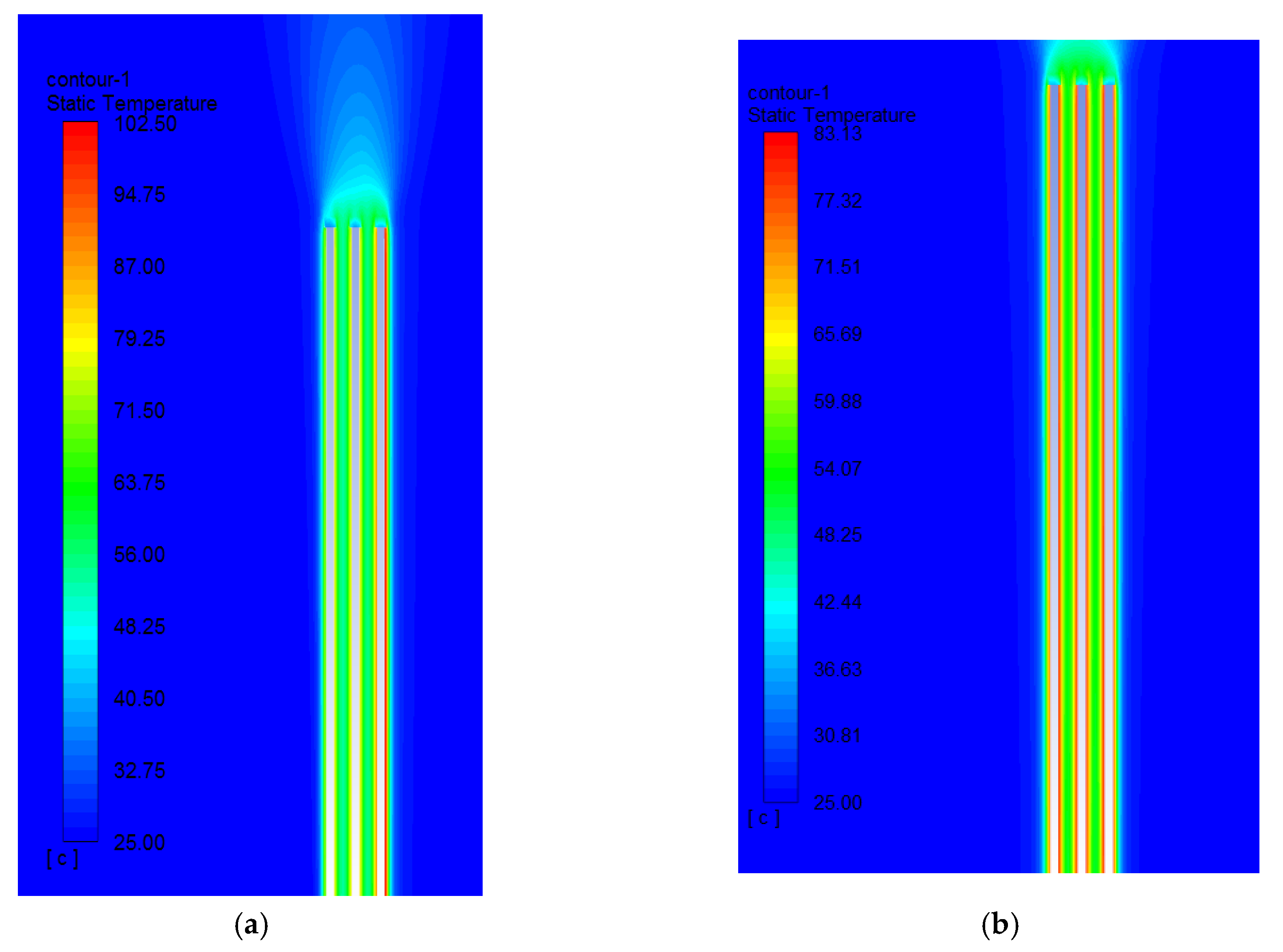
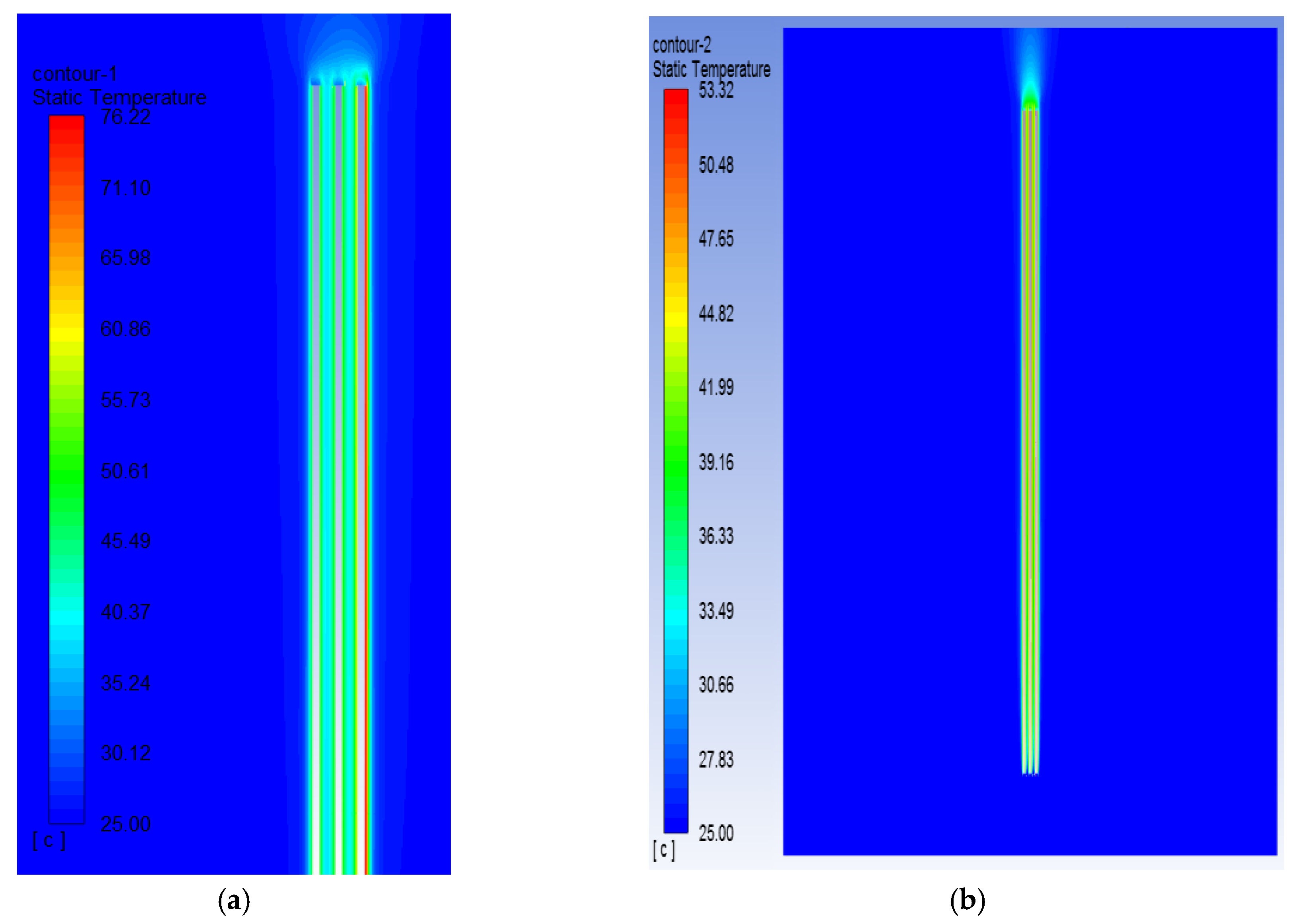
3. Computer Simulations and Results

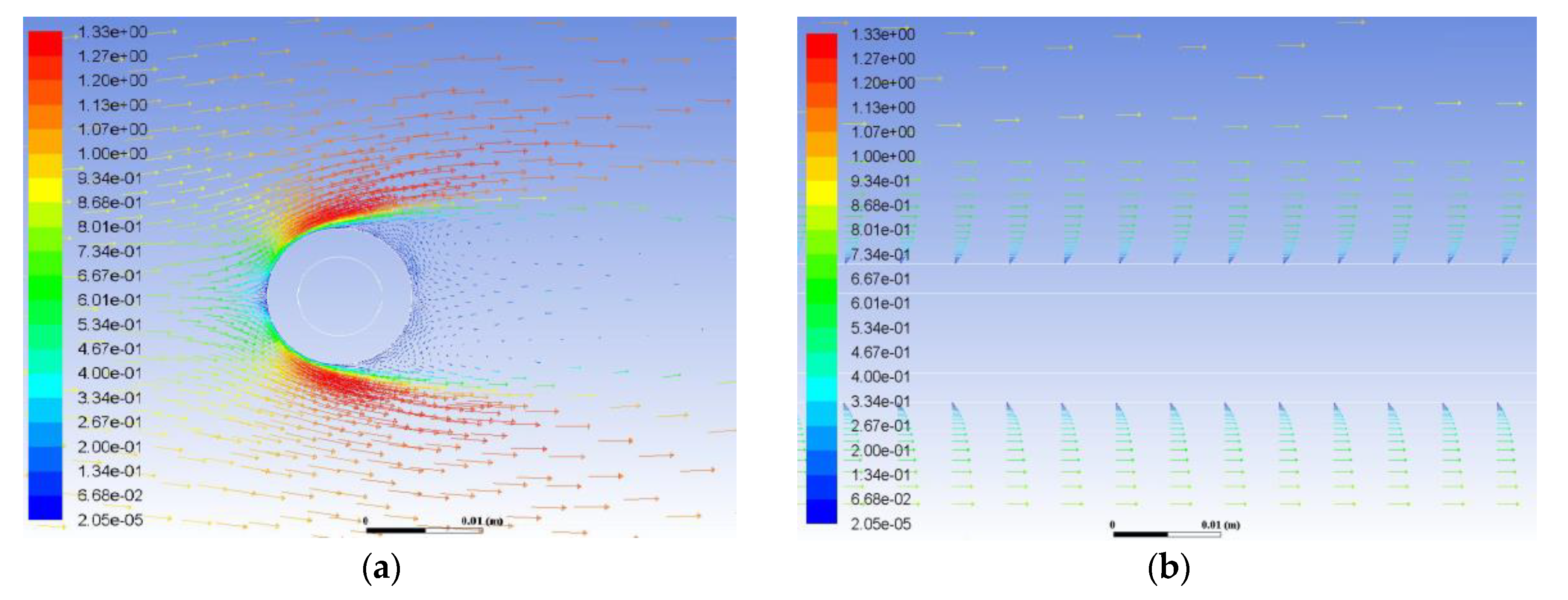
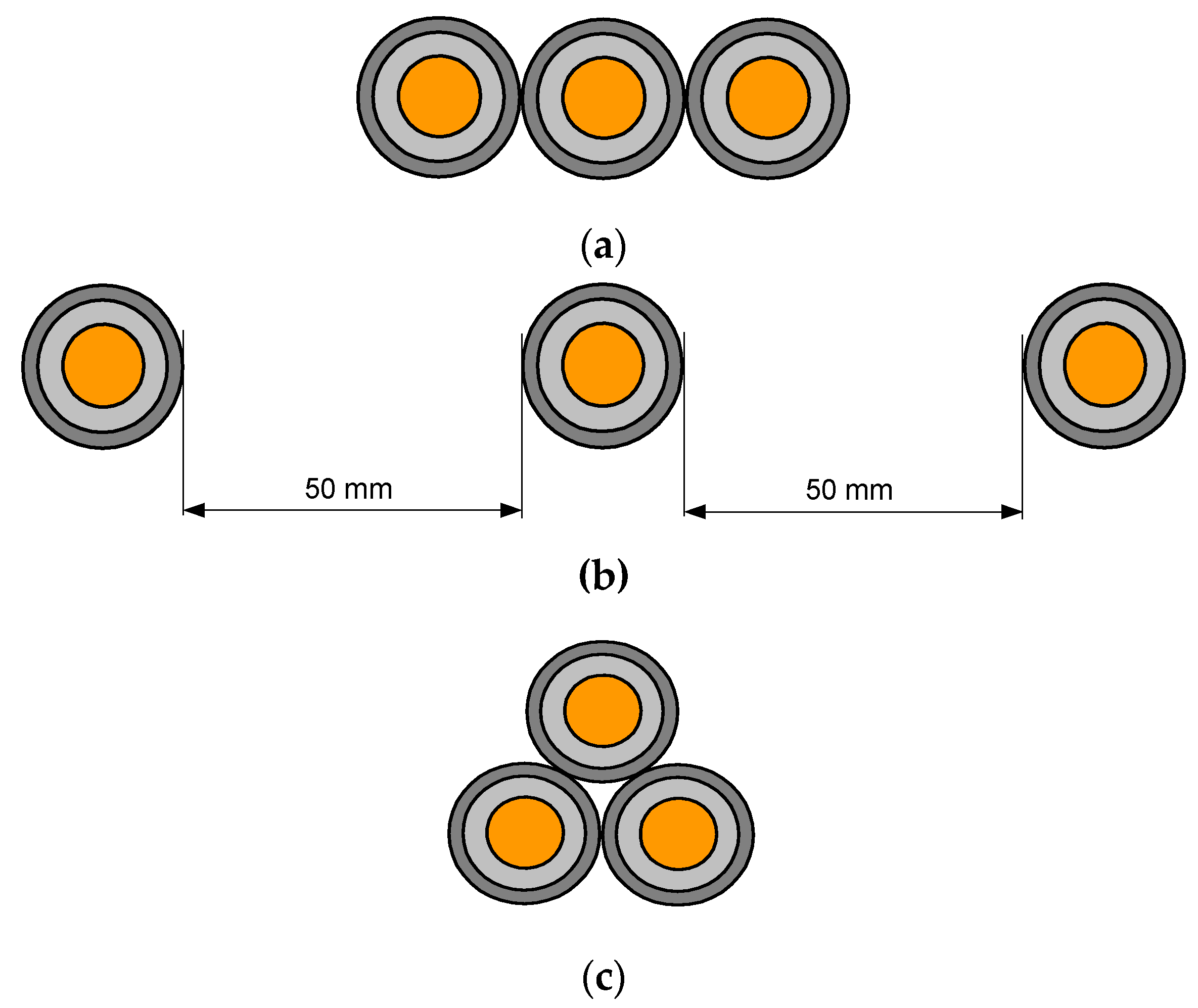
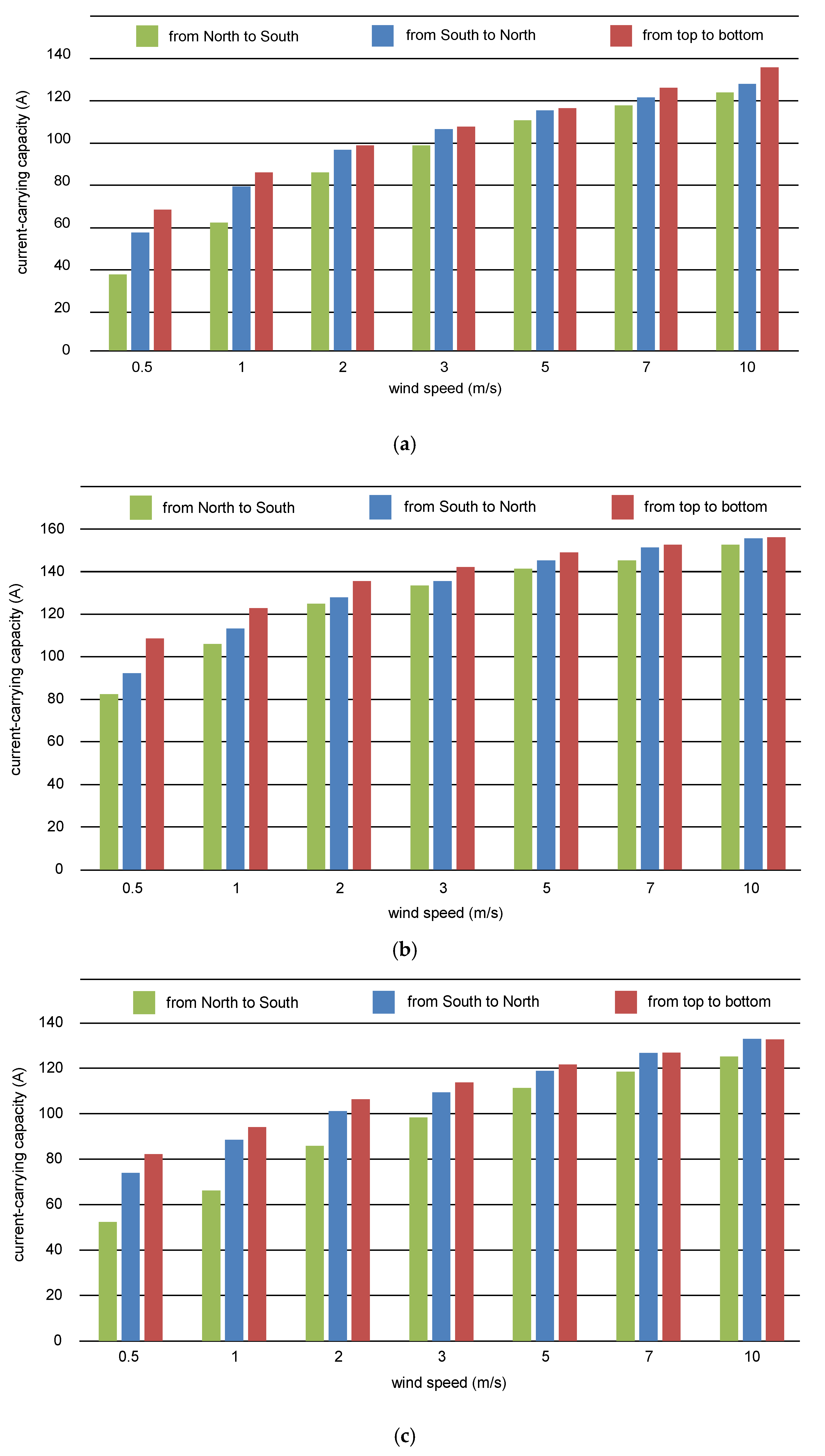
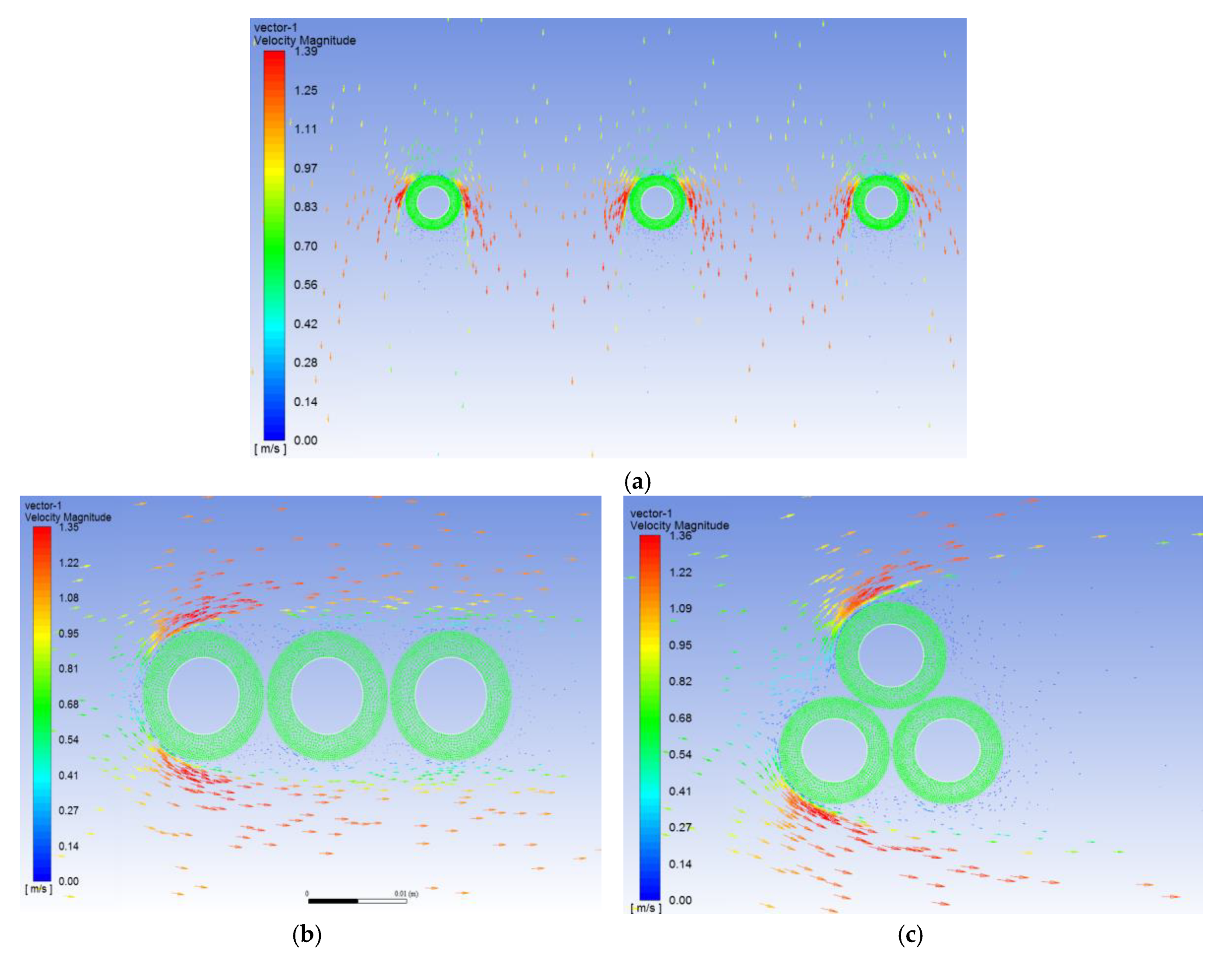
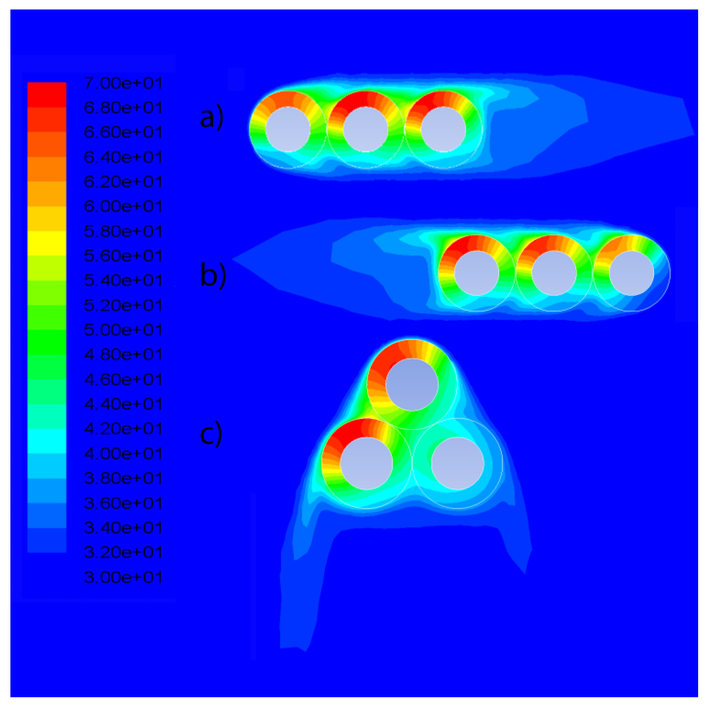
3.1. The Effect of the Wind Speed, Wind Direction and Cables Layout

In practice, the wind speed can take different directions. Usually, it will be possible to distinguish the perpendicular and parallel components in relation to the surface of the power cable. Wind directions affect the intensity of heat exchange between the cable and the environment.

Figure 3a presents vectors of air velocity flowing perpendicular to the axis of a single power cable. At the inlet on the left plane of the computational domain, speed equal to 1 m/s perpendicular to the axis of the power cable was set in the model.

Figure 3b shows the distribution of air vectors with the flow parallel to the surface of the power cable. Similar to the considerations of a cable laid perpendicular to the air flow, the set airspeed is equal to 1 m/s. The air velocity near the insulation surface (blue velocity vectors in Figure 3b) is significantly lower than the velocity at some distance from this surface. This is due to the occurrence of a boundary layer formed in the vicinity of insulation and the viscosity of air flowing around the cable shape. The heat exchange, in this case, occurs mainly by conduction in the hydraulic boundary layer.

It can be clearly seen that the air movement in close proximity to the insulation wall in the case of parallel flow (Figure 3b) is less turbulent compared to the flow perpendicular to the axis of the power cable (Figure 3a), where the laminar boundary layer is definitely thinner and there are more vortex structures in the flow.

As a result, it turns out that even with a very small path traversed along the power cable and with a similar insulation temperature (70 °C), the air in the flow parallel to the power cable axis is able to receive twice less heat than the air with a direction perpendicular to the power cable axis, at a constant direction and speed of air, and a constant air temperature [30].

The current-carrying capacity of the three-phase power cable system (cable type from Figure 1) has been analyzed for the three cables layouts presented in Figure 4. For every layout, the wind direction has been taken into account according to Figure 2. The effects of the following wind directions have been investigated:

• From North to South;
• From South to North;
• From the top to bottom of the arrangement of the cables.

Results of this analysis are presented in Figure 5. A higher wind speed leads to the increased current-carrying capacity of the cable system. However, the highest increment of this capacity is for changing the wind speed from 0.5 m/s to 1 m/s or from 1 m/s to 2 m/s. For relatively high wind speed, when the flow is already turbulent, the increase of 1 m/s is not very effective. It can also be concluded that the most intense heat exchange occurs in the case of the air flow in the top-bottom direction, compared to the direction South–North or North–South. For the top–bottom flow, comparatively higher values of the current-carrying capacity of power cables were obtained. According to this, placing a cable line vertically instead of horizontally could be a reasonable option.

If one compares the trefoil formation with the flat formation without spacing, the first of these two mentioned gives a higher current-carrying capacity of the cable line, when the wind speed is relatively low (compare Figure 5a vs. Figure 5c for the wind speed up to 2 m/s).

The best of the power cables layouts, among the analyzed ones, is the flat formation with cables spacing of 50 mm (Figure 5b). For this type of arrangement, the current-carrying capacity of the cable line is the highest (among the considered).

As the results in Figure 5 show, the speed of air inflow has a significant impact on the current-carrying capacity of power cables. This effect is particularly noticeable for the speed of 0.5–3.0 m/s. The justification for this phenomenon is the fact that the increase in the air flow velocity causes a proportional increase in the Reynolds number. According to the relationships attributed to the forced convective heat exchange, an increase in the Reynolds number results in an increase in the Nusselt number. Increasing the Nusselt number results in increasing the heat transfer coefficient α_conv. The convective heat exchange becomes the dominant method of heat exchange between the power cable and the environment.

Figure 6 presents the distribution of air velocity vectors around the cables. In Figure 6a, air velocity vectors around each power cable show vortex structures (density of velocity vectors) that intensify convective heat exchange between the cable and air. The air velocity increases to 1.39 m/s, where the set starting value is 1 m/s in the top-bottom flow. The airflow around the power cables is based on the principle that the first power cable is cooled by air like a single cable, while the next cable/cables are located in the flow structures generated by the preceding cables, as shown in Figure 6b,c. More turbulent air flow (higher air speed) leads to the more efficient convective heat transfer. Figure 6b shows the distribution of air velocity vectors for the South–North inflow (from the left to the right in the picture), where it can be seen that near the first cable (left, L1) a higher air velocity is recorded compared to the velocity distribution around the L2 and L3 cables, and therefore, locally, the heat transfer around the first (left) cable is more intense. In the trefoil formation (Figure 6c), two cables are directly exposed to the wind.

Figure 7a shows the temperature distribution in the “flat formation without spacing” case. The first power cable (left, L1) receives the highest solar heat (from the left as in Figure 2) compared to others, but it is not the hottest one. The other cables (L2 and L3) are screened by the cable L1 from the cooling effect of the wind in the direction South–North, reaching a higher temperature. In consequence, the temperature of the cables L2 and L3 determines the current-carrying capacity of the cable system. If the wind direction is changed to North–South (from the right to the left side in Figure 7b), the current-carrying capacity of the cable line is determined by the first cable (left, L1), irradiated, and the worst (last) cooled by the air stream.

When comparing the results of temperature distributions in Figure 7a,b, it is important to note that the current-carrying capacities differ by as much as 27%. For the example from Figure 7a, the current-carrying capacity (maximum permissible symmetrical load of the all cables) is equal to 78.8 A, whereas for the example in Figure 7b, the capacity is equal to 61.9 A.

Figure 7c shows an example analysis of the temperature distribution for the trefoil formation. For this type of arrangement, it is seen that the heat supplied from solar radiation to the power cable L3 (the bottom cable on the right) is significantly limited due to the shadow zone of the other cables. In case of the wind direction from top to bottom, each cable is cooled by the wind. For wind direction from South to North (from left to right), two cables at the left side of the picture are subject to wind cooling (see air velocity vectors in Figure 6c).

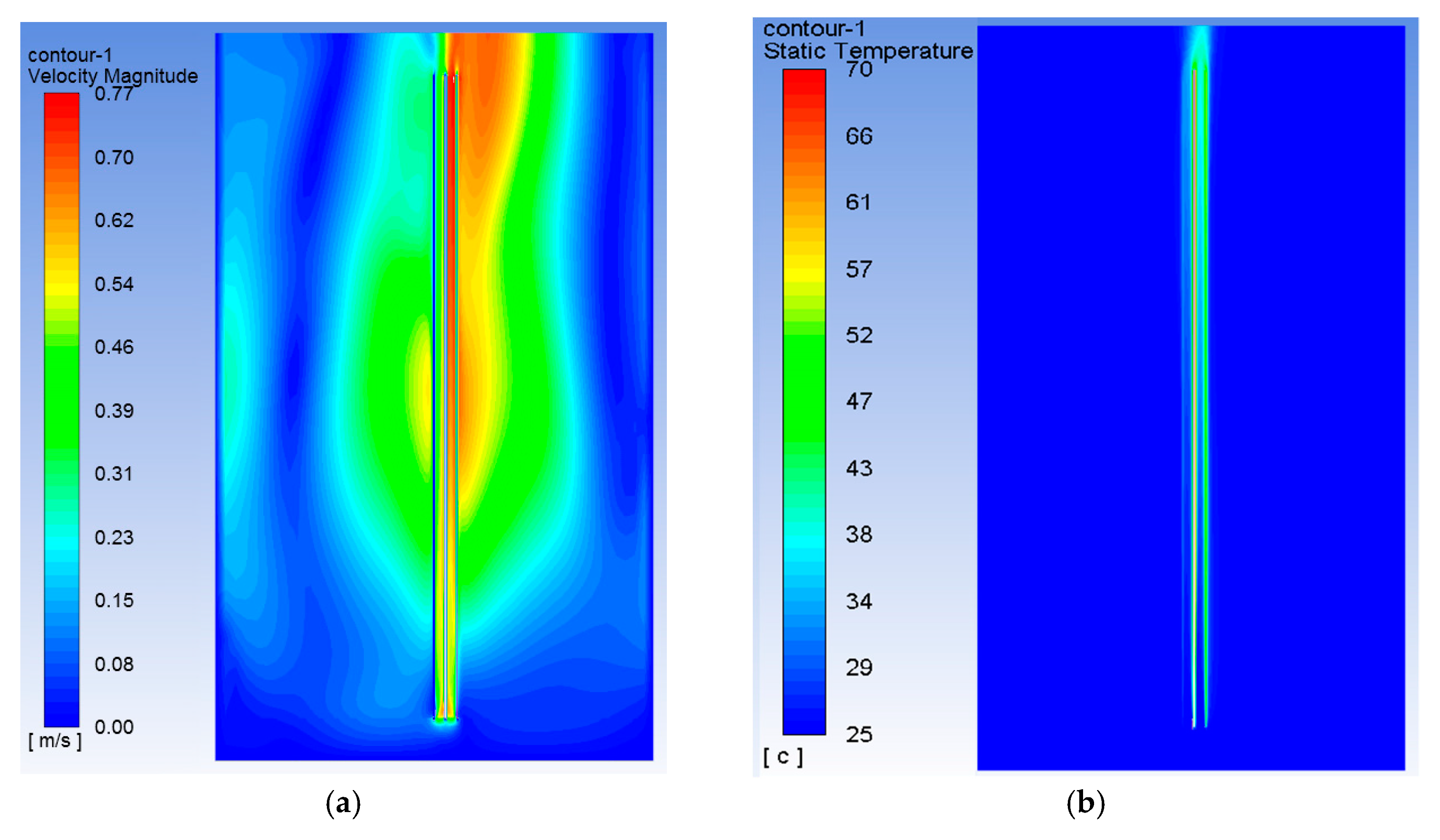
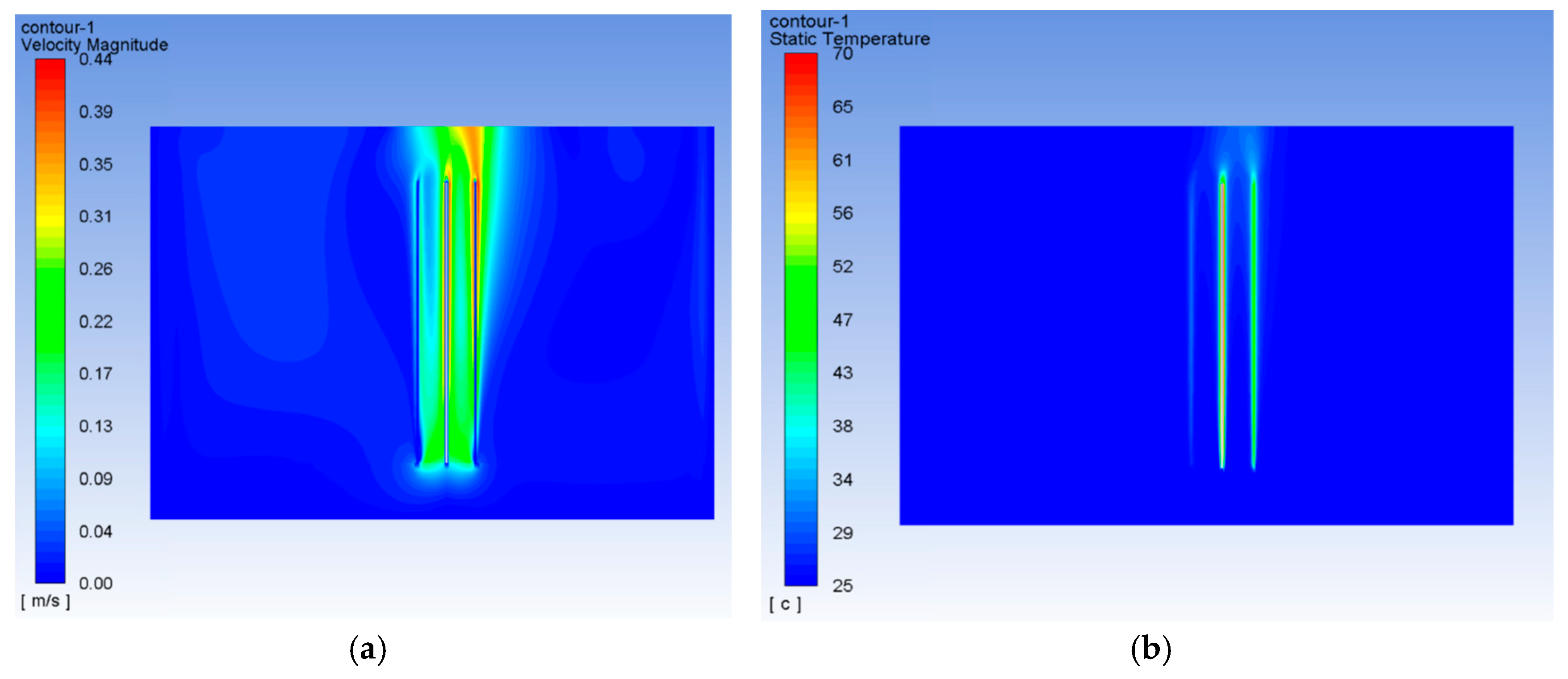
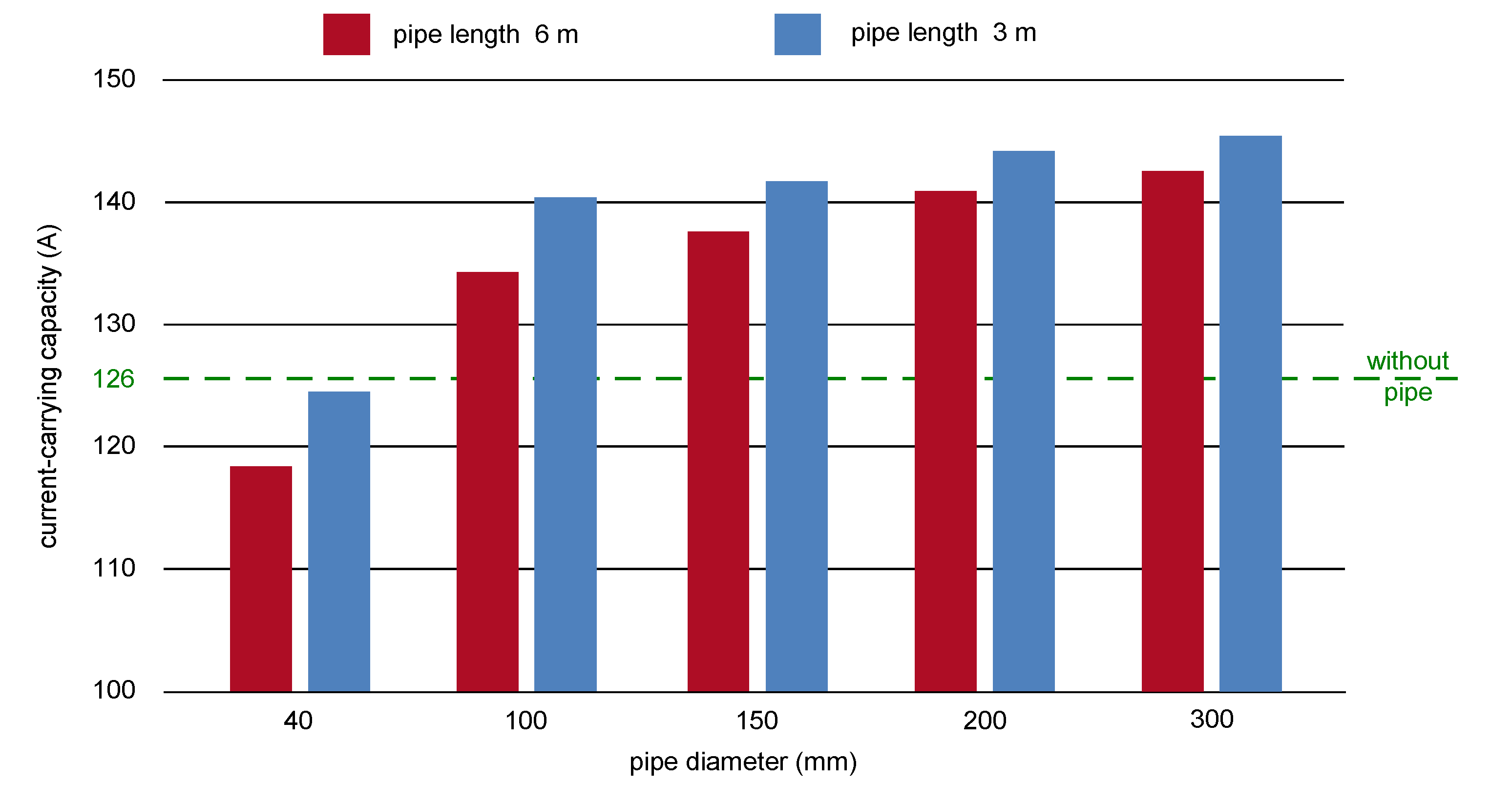
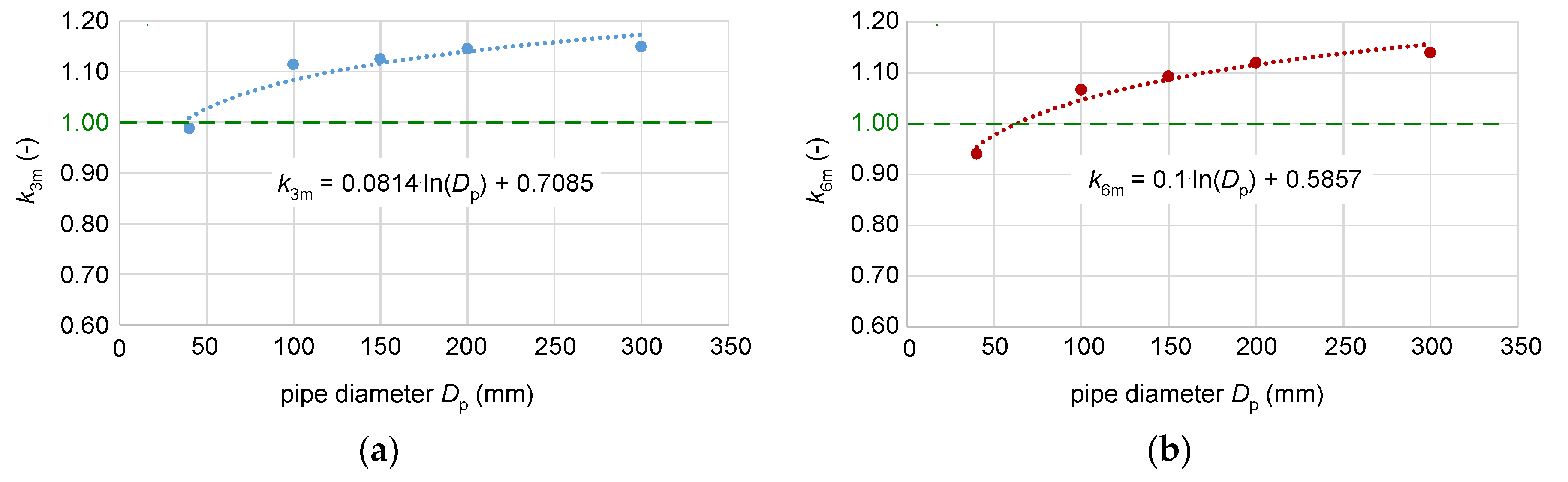
3.2. Power Cables in the Ground vs. Power Cables in Free Air

The current-carrying capacity of the power cable lines is usually calculated for cables buried in the ground. The average value of the soil thermal resistivity in many European countries (e.g., Italy, Norway, Poland) is 1.0 (K·m)/W [31]. With this in mind, the value of the current-carrying capacity for a cable line, for example, arranged in accordance with Figure 8 (if only the conditions in the ground are taken as the criterion) is 176.2 A. The results are consistent with the data contained in the standard [9].

In the further analysis, the heat flux density q_Joule determined for the current-carrying capacity of power cables located in the ground was adopted as the reference value and mapped in the above-ground part of the cable line (cables laid in free air). The insulation temperatures of cables laid in the air (without wind—unfavourable conditions) for the boundary condition q_Joule resulting from the conditions in the ground are presented in Figure 9.

Based on the results obtained in Figure 9, it can be concluded that there is a real risk of exceeding the long-term permissible temperature (70 °C) in a section of the cable line arranged in the air, both in the presence and absence of solar radiation. As a result, the reliability of the power grid is below expectations [32].

Power cables in the air cannot be loaded as much as in the ground characterized by the soil resistivity equal to 1.0 (K·m)/W. In the air, their maximum permissible load is only 96 A (with solar radiation) and 152 A (without solar radiation). Even worse, in the presence of solar radiation, the insulation of the cable may be overheated (76.22 °C—Figure 10a) for the load equal to 117.5 A, which is the current-carrying capacity of cables in the ground for the soil resistivity is equal to 2.5 (K·m)/W (relatively high soil thermal resistivity—bad heat dissipation).

In order to improve heat exchange conditions for cables laid in the air and reduce the adverse factor (solar radiation) affecting the current-carrying capacity of power cables, a method of increasing the permissible load using a passive cooling system has been proposed. The idea of the solution is based on the use of a casing/shielding pipe made of PVC, in which the power cable is laid coaxially (Figure 11). Such a pipe is usually installed for the protection of the cable/cables against mechanical damage, but it is closed at the top and its dimensions are not optimized from the point of view of thermal effects (Figure 12). If the pipe is opened at both sides and optimized, it creates a pipe-channel and can be a solution for improving the current-carrying capacity in the presence of solar radiation. The heat exchange occurring in the power cable system with the casing pipe is mainly based on the principle of free convection, in which air flow is the result of buoyancy force resulting from the difference in air density arising due to the change in air temperature in the pipe.

To illustrate physical phenomena in the arrangement “the cable in a pipe” (during solar radiation as in Figure 11), numerical simulations of natural convection around the power cable have been performed. Figure 13 presents results of these simulations for the case in which the pipe has a length of 3 m and the internal diameter is 100 mm, whereas Figure 14 presents the case with the pipe length equal to 1 m and its diameter equal to 200 mm.

Figure 15 presents the results of the numerically-based calculations of the current-carrying capacity of a single cable located in the pipe. The calculations have been performed for two lengths of the pipe (3 m and 6 m), and for pipe internal diameters 40 mm, 100 mm, 150 mm, 200 mm and 300 mm. In Figure 15, the reference current-carrying capacity, without the pipe and with solar radiation is marked as well (126 A). The key factor is the diameter of the casing pipe, because the smaller the diameter, the weaker the air movement and velocity in the pipe, so the heat exchange is difficult. A positive effect of the pipe is obtained for the pipe diameters 100 mm, 150 mm, 200 mm and 300 mm. The diameter 40 mm is too low for this cable—the current-carrying capacity is lower than for the reference case 126 A. The length of the cable is important as well. For the pipe (cable) length of 3 m and the diameter 100 mm, the current-carrying capacity is practically the same as for the length of 6 m and the diameter 200 mm.

From the considered cases, the highest current-carrying capacity (145 A) has been obtained, when a pipe of the length of 3 m and the diameter 300 mm is applied. This is around 15% more than in the case without a pipe and in the presence of solar radiation (126 A). It should be noted that the result for the pipe diameter 300 mm (length 3 m) is very similar to the case with the pipe diameter equal to 200 mm (length 3 m)—in practice, it is not necessary to increase the diameter above 200 mm. Thus, it is clearly visible that the parameters of the cable-in-pipe arrangement have to be optimized from a thermal effects point of view. Especially, since the length of the cable section in the air can be different in each case. This length influences the pipe diameter.

The authors have estimated mathematical functions, which enable the calculation of the current-carrying capacity correction factors for the case where the analyzed cable is placed in the casing pipe. Figure 16a presents the correction factor k_3m for the pipe of the length of 3 m, whereas Figure 16b presents the analogical correction factor k_6m for the pipe of the length of 6 m. The values of the correction factors are referred to the case with solar radiation and without a pipe (126 A = 1.00). Multiplying the base value (with solar radiation and without a pipe) of the current-carrying capacity by the correction factor gives the permissible load of the cable (35 mm²) in the pipe. Such mathematical functions can be helpful for power cable line designers.

4. Conclusions

Power cables located in free air can be exposed to wind and solar radiation. Both aspects significantly affect the current-carrying capacity of the cables. The riskiest configuration of the power cable line is the case in which almost the entire length of the line is buried in the ground, but at some length, it is placed in free air. In the ground, the ambient thermal conditions during the day are relatively stable. In free air, they may change extremely—from strong wind without sun to air stagnation with strong solar radiation. The modelling of such conditions, to evaluate the current-carrying of the power cables, is not an easy task.

To reflect the ambient conditions in free air, computational fluid dynamics modelling, implemented in the ANSYS software, has been used. The authors have developed an original thermal model of the cable system, which enables us to conduct advanced heat exchange analyses. Thanks to the advanced modelling and many calculations, the mixed effect of solar radiation and wind have been verified. The results of the numerical simulations presented in the paper indicate that the current-carrying capacity of the cables in air depends on the cables’ formation as well as the placement of cables in relation to the sun and wind direction, including geographical direction.

When the mixed effect of solar radiation and wind is considered, in one assumed cable arrangement (flat formation without spacing, wind 1 m/s), the current-carrying capacities may differ around 27%, depending on what the wind direction is—from North to South (61.9 A; Figure 7b) or from South to North (78.8; Figure 7a). In the modelled arrangement, the sun heats the cables from the South, so the South-facing wind gives a better cooling effect than the North-facing wind. It shows that the geographical location of the cable system, and hence the properties of that particular region of the Earth (sun altitude, dominant direction of wind) influence the current carrying-capacity of cables in free air. Such factors are not considered in the international standards; therefore, in practice, additional advanced computer modelling for the given cables arrangement can be necessary.

The evaluation of the current-carrying capacity of power cables is especially important when the underground cable line is supplied from an overhead line and goes along its pole. Unfavourable thermal conditions in free air may cause relatively high disproportions between the current-carrying capacities (ground vs. free air). To increase the capacity of cables in free air, a method for improving the thermal condition of cables, based on passive cooling and the buoyancy effect, has been proposed. In this method, the power cable is placed coaxially in a vertical pipe. Thanks to the chimney effect in such a pipe-channel, the airflow is naturally intensified and it leads to the intensification of thermal convection from the external surface of the cables. One of the most important elements of the research is the optimization of the dimensions of the channel, in order to obtain the highest increase in the power cables’ current-carrying capacity. The conducted research for the example power cable system has shown that the channel formed by the vertical pipe may give around 15% higher current-carrying capacity compared to the case without the pipe (145 A vs. 126 A). The proposed method of increasing the current-carrying capacity is economically attractive because it does not require a power supply to generate intensification of the airflow along the cables.

Results of the research presented in this paper show that for the arrangements of the power cable systems in which many factors influence the heating/cooling the cables (mainly solar radiation, wind speed, wind direction), the advanced computer simulation should be employed. What is important, every case of the cable arrangement should be considered individually. Overestimating the current-carrying capacity of cables, due to the utilization of the unified procedures included in the international standards, may result in rapid thermal damage to the cables, which is associated with additional costs.

References

- Czapp, S.; Czapp, M.; Szultka, S.; Tomaszewski, A. Ampacity of power cables exposed to solar radiation—Recommendations of standards vs. CFD simulations. E3S Web Conf. 2018, 70, 1–5. [Google Scholar] [CrossRef]
- Spyra, F. External factors influence on current-carrying capacity in an electric power cable line. Energetyka 2007, 6–7, 451–454. [Google Scholar]
- Brender, D.; Lindsey, T. Effect of rooftop exposure in direct sunlight on conduit ambient temperatures. In Proceedings of the 2006 IEEE Industry Applications Conference Forty-First IAS Annual Meeting, Tampa, FL, USA, 8–12 October 2006. [Google Scholar]
- Szpyra, W.; Kacejko, P.; Pijarski, P.; Wydra, M.; Tarko, R.; Kmak, J. Dynamic management of transmission capacity in power systems. Acta Energetica 2017, 4, 68–77. [Google Scholar]
- Czapp, S.; Szultka, S.; Tomaszewski, A.; Szultka, A. Effect of solar radiation on current-carrying capacity of PVC-insulated power cables—The numerical point of view. Tehnicki Vjesnik 2019, 26, 1821–1826. [Google Scholar]
- IEC. IEC 60287-1-1:2001. Electric Cables–Calculation of the Current Rating–Part. 1-1: Current Rating Equations (100 % load factor) and Calculation of Losses–General; International Electrotechnical Commission: Geneva, Switzerland, 2001. [Google Scholar]
- IEC. IEC 60287-2-1:2001. Electric Cables–Calculation of the Current Rating–Part. 2-1: Thermal Resistance–Calculation of the Thermal Resistance; International Electrotechnical Commission: Geneva, Switzerland, 2001. [Google Scholar]
- IEC. IEC 60287-3-1:1999. Electric Cables–Calculation of the Current Rating–Part. 3-1: Sections on Operating Conditions–Reference Operating Conditions and Selection of Cable Type; International Electrotechnical Commission: Geneva, Switzerland, 1999. [Google Scholar]
- IEC. IEC 60364-5-52:2011. Low-Voltage Electrical Installations–Part. 5-52: Selection and Erection of Electrical Equipment–Wiring Systems; International Electrotechnical Commission: Geneva, Switzerland, 2011. [Google Scholar]
- IEEE Standard Power Cable Ampacity Tables; Institute of Electrical and Electronics Engineers: Piscataway, NJ, USA, 1994.
- Neher, J.H.; McGrath, M.H. The calculation of the temperature rise and load capability of cable systems. Trans. Am. Inst. Electr. Eng. Part III: Power Appar. Syst. 1957, 76, 752–764. [Google Scholar] [CrossRef]
- De Leon, F. Calculation of Underground Cable Ampacity. CYME Int. TD: St. Bruno, QC, Canada, 2005. [Google Scholar]
- De Leon, F. Major factors affecting cable ampacity. In Proceedings of the IEEE Power Engineering Society General Meeting, Montreal, QC, Canada, 18–22 June 2006. [Google Scholar]
- Du, Y.; Burnett, J. Current distribution in single-core cables connected in parallel. IEEE Proc.-Gener. Transm. Distrib. 2001, 148, 406–412. [Google Scholar] [CrossRef]
- Baazzim, M.S.; Al-Saud, M.S.; El-Kady, M.A. Comparison of Finite-Element and IEC methods for cable thermal analysis under various operating environments. Int J. Elect Robot. Electron. Commun Eng. 2014, 8, 470–475. [Google Scholar]
- Xu, X.; Yuan, Q.; Sun, X.; Hu, D.; Wang, J. Simulation analysis of carrying capacity of tunnel cable in different laying ways. Int. J. Heat Mass Transf. 2019, 130, 455–459. [Google Scholar] [CrossRef]
- Sedaghat, A.; Lu, H.; Bokhari, A.; De Leon, F. Enhanced thermal model of power cables installed in ducts for ampacity calculations. IEEE Trans. Power Deliv. 2018, 33, 2404–2411. [Google Scholar] [CrossRef]
- Xiong, L.; Chen, Y.; Jiao, Y.; Wang, J.; Hu, X. Study on the Effect of cable group laying mode on temperature field distribution and cable ampacity. Energies 2019, 12, 3397. [Google Scholar] [CrossRef]
- Makhkamova, I.; Taylor, P.C.; Bumby, J.R.; Mahkamov, K. CFD Analysis of the Thermal State of an Overhead Line Conductor. In Proceedings of the 43rd International Universities Power Engineering Conference, Padova, Italy, 7 September 2008; pp. 1–4. [Google Scholar]
- Makhkamova, I.; Mahkamov, K.; Taylor, P.C. CFD thermal modelling of Lynx overhead conductors in distribution networks with integrated renewable energy driven generators. Appl. Therm. Eng. 2013, 58, 522–535. [Google Scholar] [CrossRef]
- Zeńczak, M. Approximate Relationships for Calculation of Current-Carrying Capacity of Overhead Power Transmission Lines in Different Weather Conditions. In Proceedings of the Progress in Applied Electrical Engineering (PAEE), Koscielisko, Poland, 25–30 June 2017. [Google Scholar]
- Liang, K.; Li, Z.; Chen, M.; Jiang, H. Comparisons between heat pipe, thermoelectric system, and vapour compression refrigeration system for electronics cooling. Appl. Therm. Eng. 2019, 146, 260–267. [Google Scholar] [CrossRef]
- Staton, D.A.; Cavagnino, A. Convection Heat Transfer and Flow Calculations Suitable for Analytical Modelling of Electric Machines. In Proceedings of the 32nd Annual Conference on IEEE Industrial Electronics, Paris, France, 6–10 November 2006; pp. 4841–4846. [Google Scholar]
- Amr, A.A.; Hassan, A.A.M.; Abdel-Salam, M.; El-Sayed, A.H.M. Enhancement of photovoltaic system performance via passive cooling. In Proceedings of the Nineteenth International Middle East Power Systems Conference (MEPCON), Cairo, Egypt, 19–21 December 2017; pp. 1430–1439. [Google Scholar]
- Bădălan, N.; Svasta, P. Fan vs. passive heat sink with heat pipe in cooling of high power LED. In Proceedings of the IEEE 23rd International Symposium for Design and Technology in Electronic Packaging (SIITME), Constanta, Romania, 26–29 October 2017; pp. 296–299. [Google Scholar]
- Dupont, V.; Billet, C.; Nicolle, T. High performances passive two-phase loops for power electronics cooling. In Proceedings of the International Exhibition and Conference for Power Electronics, Intelligent Motion, Renewable Energy and Energy Management, Nuremberg, Germany, 10–12 May 2016. [Google Scholar]
- Imburgia, A.; Romano, P.; Chen, G.; Rizzo, G.; Sanseverino, E.R.; Viola, F.; Ala, G. The industrial applicability of PEA space charge measurements for performance optimization of HVDC power cables. Energies 2019, 12, 4186. [Google Scholar] [CrossRef]
- Andersen, S.A. Automatic Refrigeration; MacLaren for Danfoss: Nordborg, Denmark, 1959. [Google Scholar]
- Modest, F.M. Radiative Heat Transfer, 3rd ed.; Academic Press: Cambridge, MA, USA, 2013. [Google Scholar]
- Czapp, S.; Szultka, S.; Tomaszewski, A. CFD-based evaluation of current-carrying capacity of power cables installed in free air. In Proceedings of the 18th International Scientific Conference on Electric Power Engineering (EPE), Kouty nad Desnou, Czech Republic, 17–19 May 2017; pp. 692–697. [Google Scholar]
- Czapp, S.; Ratkowski, F. Effect of soil moisture on current-carrying capacity of low-voltage power cables. Przeglad Elektrotechniczny 2019, 95, 154–159. [Google Scholar] [CrossRef]
- Chojnacki, A.Ł. Analysis of reliability of low-voltage cable lines. Przeglad Elektrotechniczny 2017, 93, 14–18. [Google Scholar]
© 2020 by the authors. Licensee MDPI, Basel, Switzerland. This article is an open access article distributed under the terms and conditions of the Creative Commons Attribution (CC BY) license (http://creativecommons.org/licenses/by/4.0/).
Share and Cite
Czapp, S.; Szultka, S.; Tomaszewski, A. Design of Power Cable Lines Partially Exposed to Direct Solar Radiation—Special Aspects. Energies 2020, 13, 2650. https://doi.org/10.3390/en13102650
Czapp S, Szultka S, Tomaszewski A. Design of Power Cable Lines Partially Exposed to Direct Solar Radiation—Special Aspects. Energies. 2020; 13(10):2650. https://doi.org/10.3390/en13102650
Chicago/Turabian StyleCzapp, Stanislaw, Seweryn Szultka, and Adam Tomaszewski. 2020. "Design of Power Cable Lines Partially Exposed to Direct Solar Radiation—Special Aspects" Energies 13, no. 10: 2650. https://doi.org/10.3390/en13102650
APA StyleCzapp, S., Szultka, S., & Tomaszewski, A. (2020). Design of Power Cable Lines Partially Exposed to Direct Solar Radiation—Special Aspects. Energies, 13(10), 2650. https://doi.org/10.3390/en13102650