1. Introduction
Tidal current energy, as a promising renewable energy type, has gained much more attention in recent years. A tidal current turbine (TCT), developed from a wind turbine, has a high ability to harness tidal current energy and is one kind of tidal energy converter that has been widely researched and developed around the world. However, TCTs often suffer from much larger axial loads than wind turbines because they work in a fluid with about a thousand times the density of air. This heavy axial load may induce a series of problems, such as blade failure, much larger driving torque of the pitch system, reduced reliability of the tower and anchor system, and so on. Hence, the blade should be strong enough to resist severe loads or have a special structure to relieve loads. Generally, the blades are designed with large margins to guarantee strength, such as by choosing a robust airfoil. In this way, more material will be needed, and the cost will then rise. One possibility to solve the problem is by reducing the load of the rotor using an advanced blade design.
The classic method to design a blade always takes into account the hydrodynamics and structure separately. Hydrodynamic design aims toward high efficiency and is followed by blade structure design based on the load distribution along the blade. Manual iterations are needed to get satisfactory results. In general, the method is more like a complicated trial-and-error and time-costly iteration process. One practical way to address this is to combine the hydrodynamic design and structure design together, i.e., hydrodynamics and structure co-design. As seen in the literature, Nicholls-Lee et al. developed a bending–twist coupled blade design method, where the axial thrust could be reduced by 12% with bending and twist deformation of the blade under the bending moment [
1,
2]. Lee and VanZwieten presented an individual pitch control method to reduce the load variation induced by flow shear [
3]. Despite its high efficiency, the actuator was complicated. In addition, Arnold et al. proposed a speed control approach for load reduction of fixed-pitch TCTs by regulating the tip speed ratio [
4]. Similar research was also reported in some other publications [
5,
6,
7].
In the above research, extreme load was relieved by blade deformation, pitch system action, or a control strategy. However, due to the nonlinearity of interaction between the flow and blade structure and the flow turbulence, the structure would be subjected more often to fluctuating fatigue load. Further, higher requirements would be placed on the blade fabrication process. Considering the complex interaction between the blade and flow, this may be a good way to combine hydrodynamic design with the optimization of the blade structure.
This combination work can be done by a computer optimization program [
8]. In a general optimization process where the goal is to find one or several extrema, the extremum can be the maximum of the power coefficient, maximum of annual power generation, minimum of the cost of energy (COE), or something else, according to different objectives. For example, the annual power generation and COE were chosen as two objectives by Benini and Toffolo [
9] and have been widely used in the wind energy field. Besides this, Noruzi et al. adopted a blade element momentum (BEM)-based iteration method to design the initial blade airfoil. Related parameters of the blade, like blade length and twist angle distribution, were optimized by comparative analysis with the computational fluid dynamics (CFD) result, thus improving the blade efficiency [
10]. Mohammadi et al. carried out the optimal hydrofoil design of hydrokinetic turbine for the low-speed current. Particle swarm optimization and XFoil were coupled to improve the hydrodynamic performance [
11]. A numerical optimization scheme using a gradient-based algorithm was proposed for the airfoil design of tidal turbines in [
12]. It used the RFOIL solver and composite Bezier geometrical parameterization. However, a global optimal solution cannot be guaranteed in such gradient-based quadratic programming.
In this paper, the co-design of hydrodynamics and structure is researched with the aim to decrease the redundancy in conventional structure design on the premise of sufficient structural strength and reduced load to prolong the blade life without sacrificing power efficiency. In this optimization design, the non-dominated sorting genetic algorithm II (NSGA-II) is employed as a multi-objective optimization algorithm, in which chord length, twist angle, and blade thickness are the optimization parameters, and maximum power coefficient and fatigue life are the optimization objectives. When the iteration process converges, the value of the obtained Pareto solution set is the optimal result for the design variables. Additionally, an equivalent S–N curve model and a simplified load spectrum are proposed based on the BEM theory for quick fatigue life estimation to avoid the time-costly iterations in traditional blade design.
The remainder of this paper is organized as follows. In
Section 2, an equivalent S–N curve model of the blade is proposed to estimate the fatigue life of the blade as a parameter of reliability and load. In
Section 3, a simplified load spectrum is presented, including the loading cycle caused by shear flow and turbulence during power production conditions. In
Section 4, an outline of the employed multi-objective genetic algorithm and detailed optimizing procedures are presented. In
Section 5, the Pareto front resulting from the optimization is first provided. Comparisons between the original design and optimal designs by both GH-bladed and ANSYS are analyzed and discussed. In the final section, conclusions are given.
3. Simplified Load Spectrum
During operation, TCT blades will experience hydrodynamic load, centrifugal load, gravitational load, etc., which are related to turbine working conditions such as power production, normal stop, start, emergency stop, grid faults, and so on. In this work, we focus on the hydrodynamic bending moments on the blades. Other loads could be dealt with in a similar way. Such a simplification would be beneficial to the understanding of optimization.
The simplified load spectrum includes the flap-wise bending moment cycle caused by shear flow and turbulence. Instead of using a Weibull distribution [
16], the current velocity data used to derive the load spectrum were measured using an acoustic Doppler velocimeter at the TCT site of Zhejiang University in Zhoushan, Zhejiang Province, China [
17].
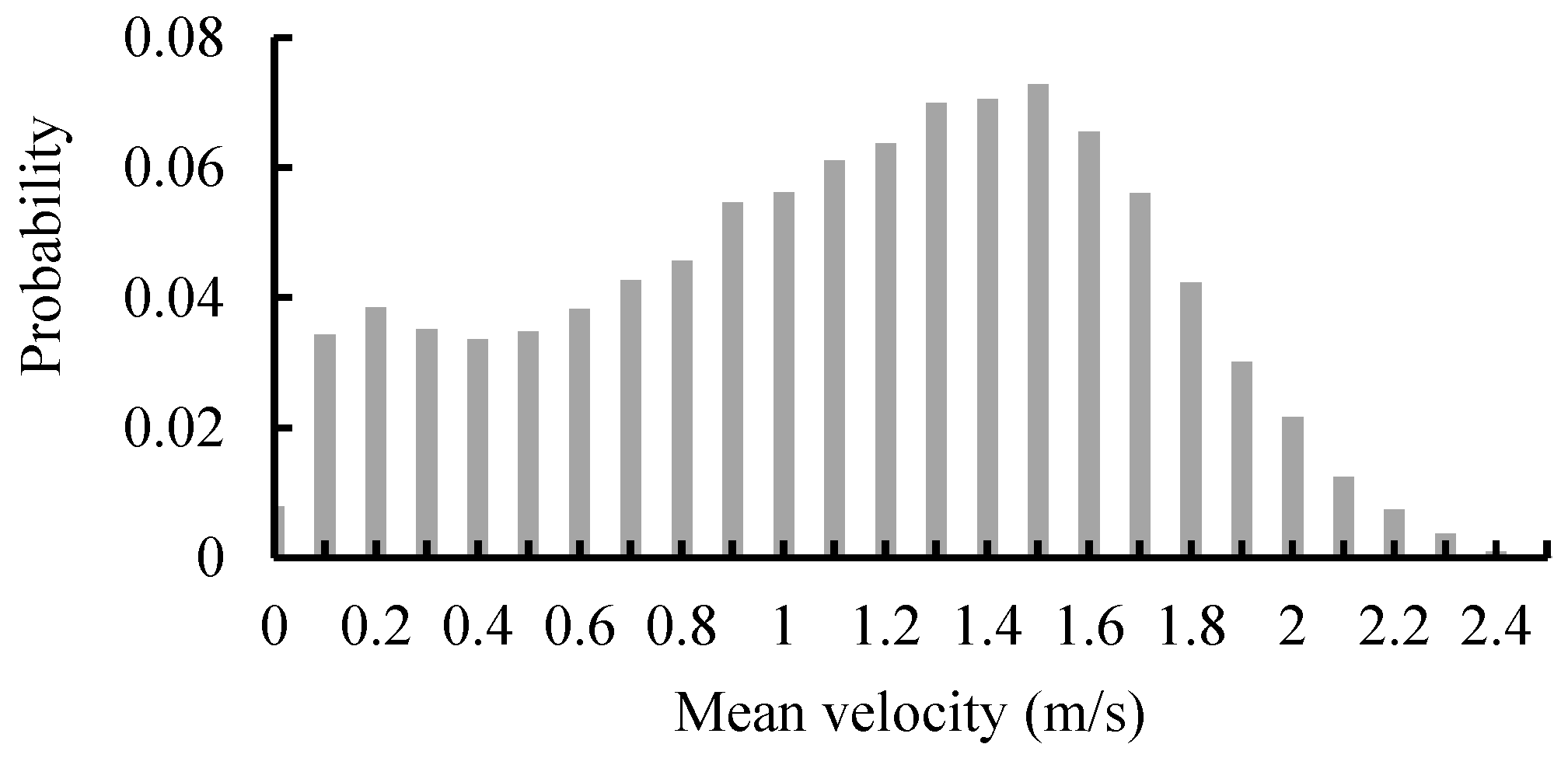
Figure 4 shows the current velocity statistics that cover data obtained over more than one year. This figure is based on bulk data statistics of the TCT site. Considering the high predictability, periodicity, and continuity of a specific flow field, a probability distribution with sufficient
x-axis resolution can mostly reflect the variation rule of the current velocity.
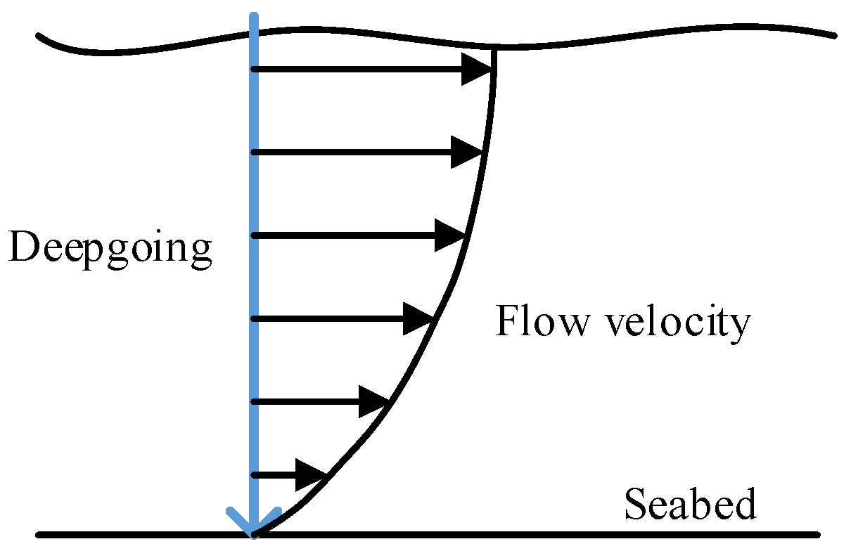
3.1. Load Cycle Caused by Shear Flow
Shear flow is a phenomenon caused by the viscosity of seawater, wherein the adjacent flow layers move parallel to each other with different velocities, as shown in
Figure 5. The flow layer near the sea surface has maximum current velocity, and the velocity drops off as it goes deeper. Such a phenomenon can be described by Equation (13) [
18].
where
v(
z) is the current velocity at depth
z,
is the current velocity at the sea surface,
d is the sea depth, and
δ is the shear exponent. At the TCT site, the sea depth is 20 m, and the shear exponent was set to be 1/7 according to in situ observations.
As the blade rotates, the current velocity varies at the blade position. When the blade moves to the 12 o’clock position, it is subject to maximum current velocity, with minimum current velocity at the 6 o’clock position. The cycle of current velocity leads to a cycle of axial load, and the axial load fluctuates at the frequency of the rotor rotating speed.
The BEM theory is used to predict the axial load when the hydrodynamic design is finished. The current velocity at a blade section location could be derived from the shear flow equation as
where
is the current velocity at a blade element,
dhub is the depth of the hub,
r is the radius of the blade element, and
is the azimuth angle of the blade.
The axial force on a blade element could be derived as the following equation:
where
dT is the axial force of the blade element, and
a is the axial induction coefficient, which can be derived as
where
B is the number of blades,
c is the local chord length,
ϕ is the inflow angle,
F is the tip loss factor [
16], and
CL and
CD are the lift and drag coefficients, respectively [
19].
The flap-wise bending moment can be derived from the axial load integral of the blade elements as
where
M is the flap-wise bending moment and
R is the radius of the rotor.
Equation (17) indicates that the bending moment is a function of
and
; thus, the cycle amplitude of the bending moment could be described by the following equation.
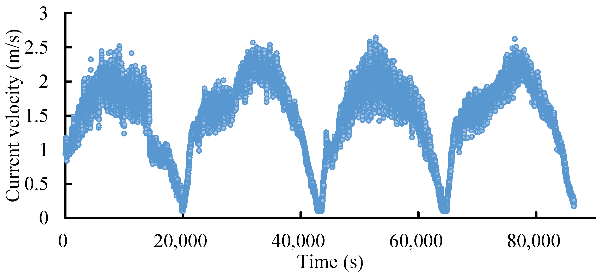
3.2. Load Cycle Caused by Turbulence
Turbulence is a phenomenon wherein the current velocity changes chaotically. Such changeable fluctuation of the current velocity will lead to fluctuation of the axial load. The intensity of turbulence can be statistically described as the standard deviation of the 10-min current velocity divided by the 10-min mean current velocity. Considering the periodicity of tidal currents, 21 turbulence samples were picked with mean velocity varying from 0.5 m/s to 2.5 m/s. For convenience in the damage equivalent load calculation, the turbulences at different velocities were fitted.
Figure 6 displays the tidal current velocity data for an entire day, detected once per second at the Zhejiang University TCT site.
Figure 7 shows the turbulence intensity statistics of the variable current velocity at this operating site.
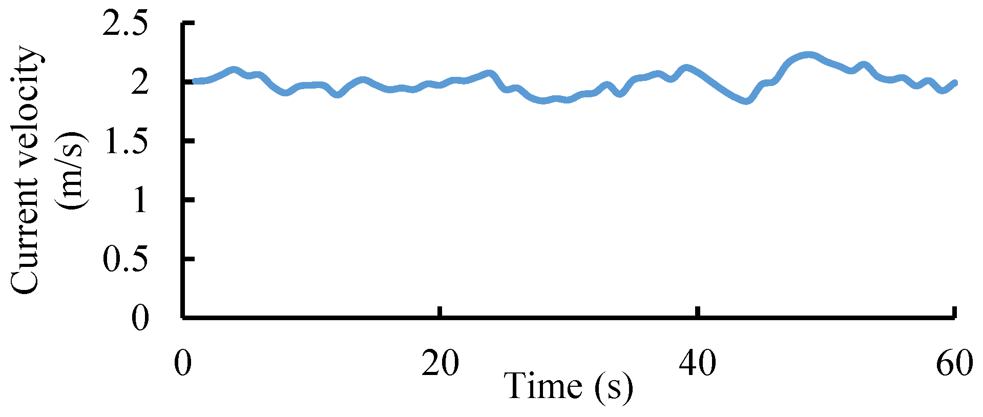
To simplify the computation, turbulence samples were used in the optimization code instead of the entire velocity dataset. Firstly, the annual velocity data were divided into fragments with length 60 s. Secondly, the fragments were picked out as the turbulence samples. In all, 21 turbulence samples were picked with mean velocity varying from 0.5 m/s to 2.5 m/s.
Figure 8 shows one of the turbulence samples with a mean velocity of 2 m/s and sampling frequency of 1 Hz. Then, a rain-flow counting algorithm was applied to count the current velocity cycle in the turbulence sample [
20].
Table 2 gives 16 velocity cycles counted from the turbulence sample. In addition, the probability of 2 m/s is 2.17% according to the probability distribution of current velocity in
Figure 4. This means that the annual occurrence of this velocity cycle in
Table 2 is 11,387 min in an annual period.
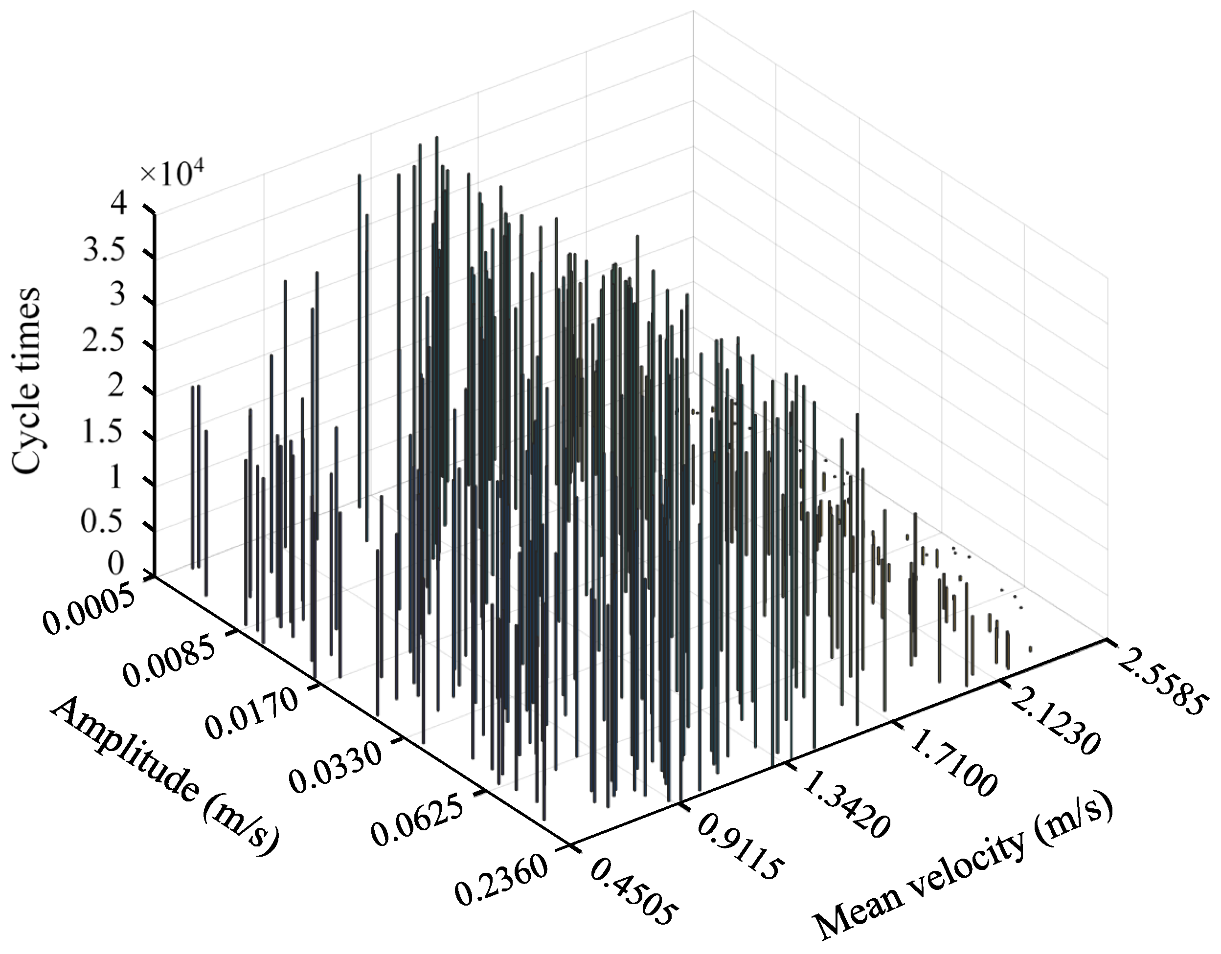
By applying the rain-flow counting algorithm to other turbulence samples, the annual statistics of velocity cycles were obtained as shown in
Figure 9, in which the height of the bar indicates the annual occurrence.
The load cycle caused by the velocity fluctuation could be described as the following equations.
where
is the amplitude of the velocity cycle, and
is the mean velocity.
4. Multi-Objective Optimization
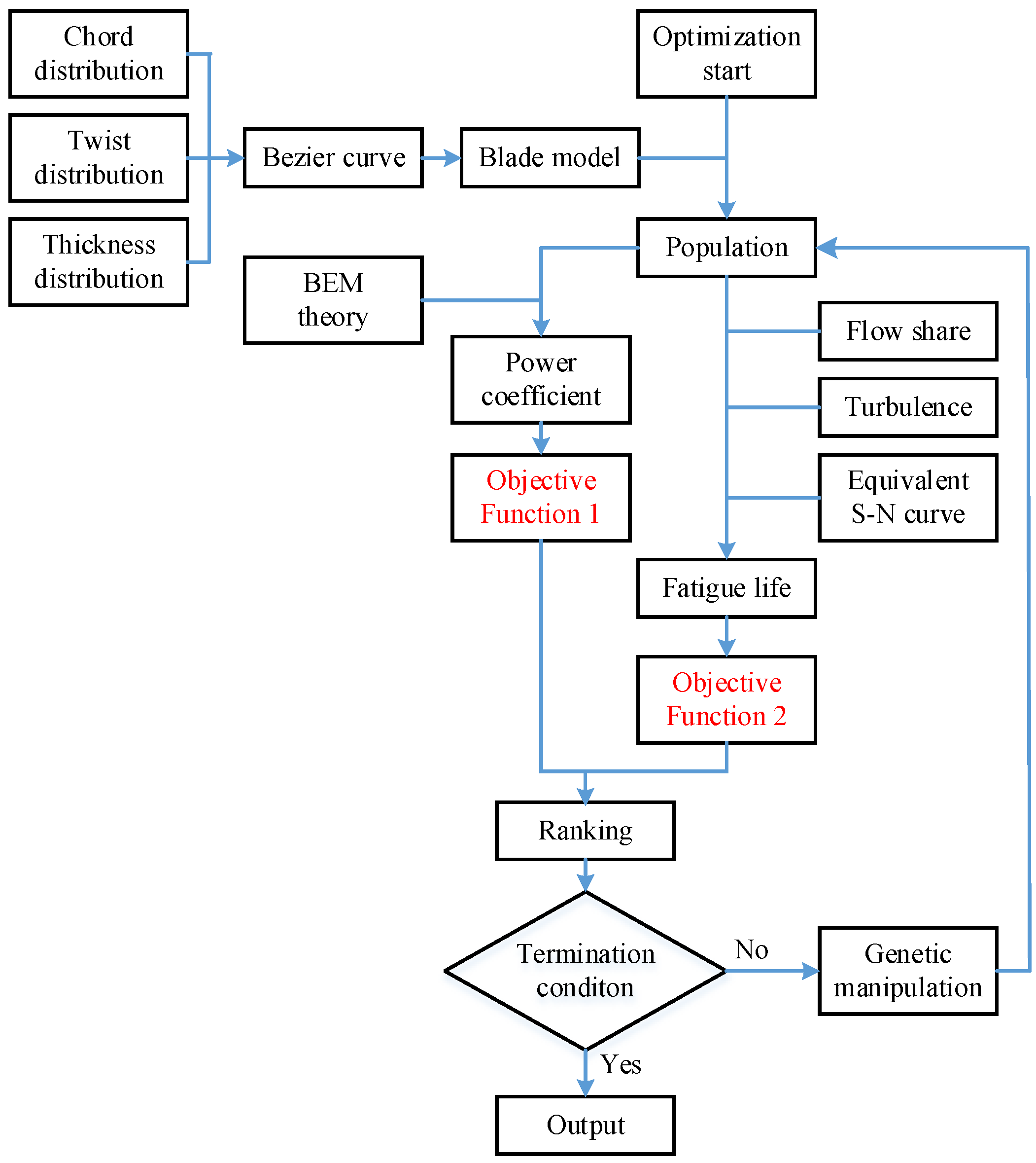
Based on the above analyses and models, a multi-objective genetic algorithm was used in the blade optimization design. The NSGA-II algorithm was employed as the multi-objective optimization algorithm. The approach to realize this blade optimization can mainly be presented as the following four steps:
Randomly initializing a population with N individuals whose attribute values should be the optimization objective parameters, such as chord length, twist angle, and blade thickness.
Calculating the power coefficient and fatigue life for each child individual, then non-dominated sorting and calculating the crowding degree on the calculated power coefficient and fatigue life.
Merging the parent and child individuals and non-dominated sorting them to obtain a new child generation.
Iterating the above steps until the termination condition, to get the Pareto solution set which includes the optimized parameter values of chord length, twist angle, and blade thickness.
The blade model can be described by three curves, namely, the chord, twist angle, and thickness distributions, in the optimization carried out on the 4.4 m TCT blade. These three distributions are fitted as Bezier curves to guarantee smoothness and to reduce the optimization parameters. An
nth-order Bezier curve can be described as the following equation.
where
Pi refers to a control point. The order of the Bezier curve depends on the complexity of the distribution. In this case, the chord, twist angle, and thickness distributions were fitted as seventh-order, fifth-order, and sixth-order Bezier curves, respectively. In total, 21 optimization parameters were used to describe a blade: 8 chord, 6 twist angle, and 7 thickness parameters.
An optimal power coefficient was determined as the first objective function, supposing that the turbine operates in the vicinity of the optimal tip speed ratio in spite of the variable velocity. The optimization concerns the magnitude and frequency of the load cycle. Although a constant tip speed ratio was used for the power efficiency optimization, the current velocity used to calculate the tip speed ratio varies due to the shear flow and turbulence. So, the current velocity at the hub location was used for the controller when calculating the axial load cycle caused by shear flow. Additionally, mean current velocities were used for the controller while dealing with the turbulence.
The hydrofoils used at each blade section were optimized based on an existed hydrofoil pool. There were altogether seven standard hydrofoils in the pool, the respective thicknesses of which were 100%, 40%, 35%, 30%, 25%, 21%, and 16%. The lift and drag coefficients of a section with arbitrary thickness were interpolated using standard hydrofoils. The blade optimization schematic is shown in
Figure 10.
In Objective Function 1, the power coefficient can be described as
where
ω is the rotating speed of the rotor under the optimal tip speed ratio.
P refers to an instantaneous value of power at each rotor azimuth angle of a rotating cycle, which is calculated by the blade element power with the consideration of flow shear and turbulence. Hence, the numerator in Equation (22) refers to the average power in a full revolution. And, the rated value of current velocity
v is generally used for the denominator to simplify the code.
P is a complicated integral in the program, the function could be described as
In Objective Function 2, the fatigue life can be described as
where
Damage refers to the accumulated damage,
ni is the cycle number of load at current velocity
vi.
Through the above optimization method, the maximum CP and minimum Damage could be found by using the genetic algorithm. In mathematical terms, the multi-objective optimization problem can be briefly formulated as follows:
min(1/CP(x), Damage(x))
such that
where set X is the feasible set of the blade structure.
Consequently, this multi-objective optimization can be done via the Matlab GA tool.
5. Results and Discussion
In
Figure 11, the Pareto front obtained by the multi-objective genetic algorithm is presented, in which each data point represents a blade design candidate. The original design is also marked. As illustrated, the original design point of the blade has high efficiency but with a fatigue life much shorter than the required lifetime of 20 years, which is mainly induced by higher axial thrust.
Two solutions in
Figure 11 were chosen to be the objects of comparative analysis as the optimal designs from the Pareto front. The first one, Optimal design 1, has a fatigue life of 20 years. The second one, Optimal design 2, has the same efficiency as the original design but a longer fatigue lifetime. For these two representative points on the Pareto solution curve, the detailed data are compared in
Table 3.
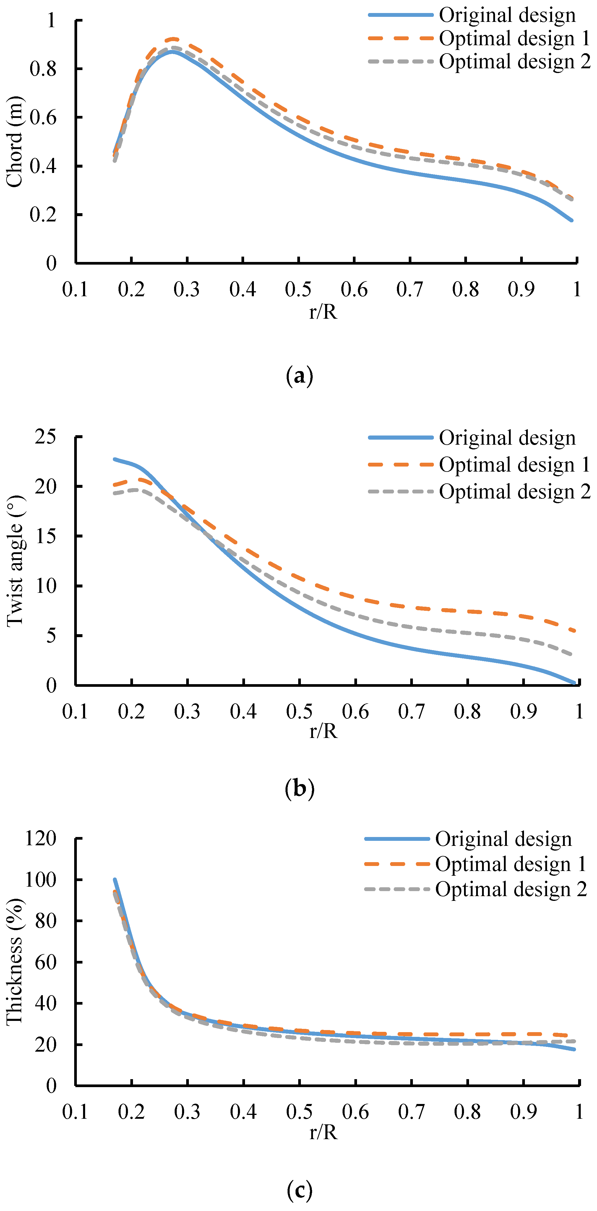
The chord length, twist angle, and thickness distributions of these three design points are presented in
Figure 12. From the figures, the chord and twist angle of the optimal designs show great improvement, while the difference in thickness is unnoticeable.
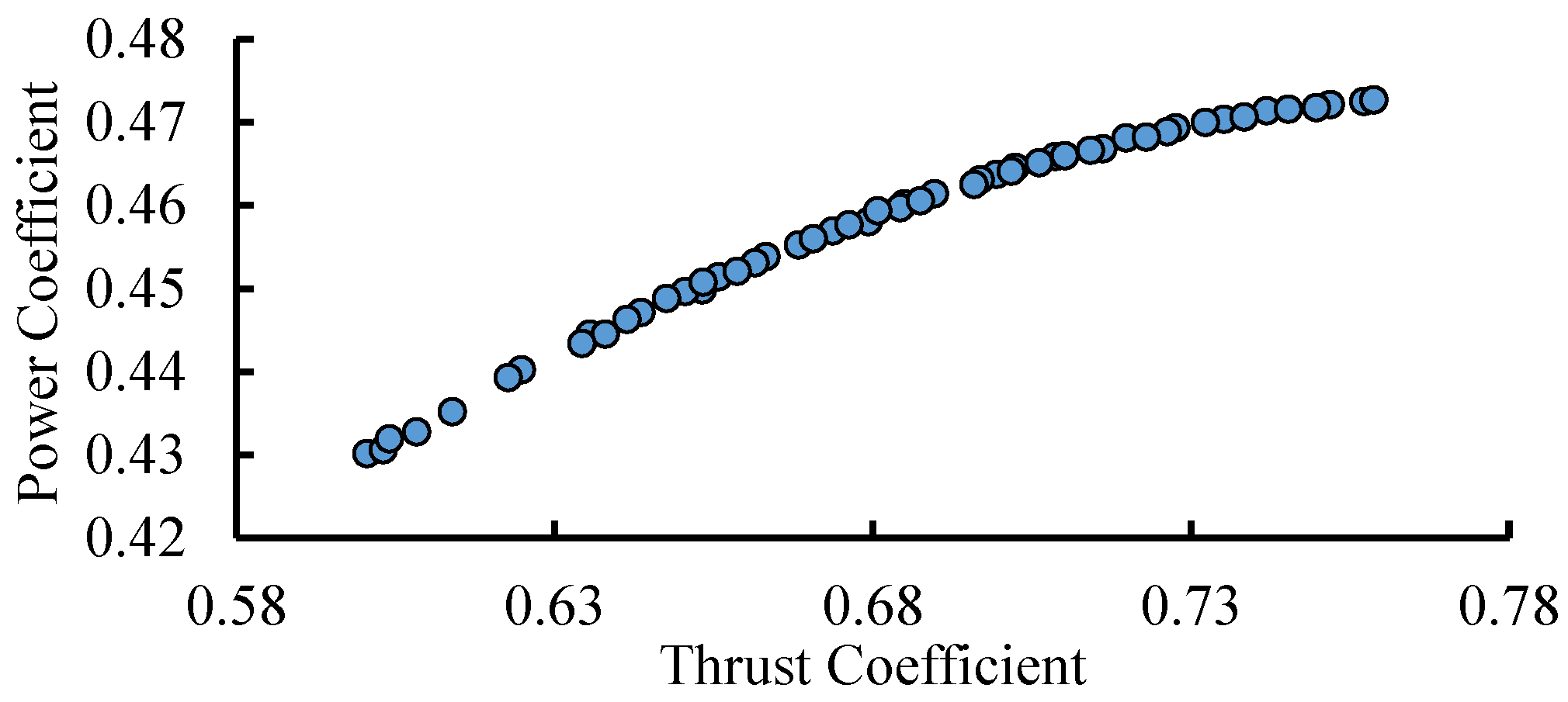
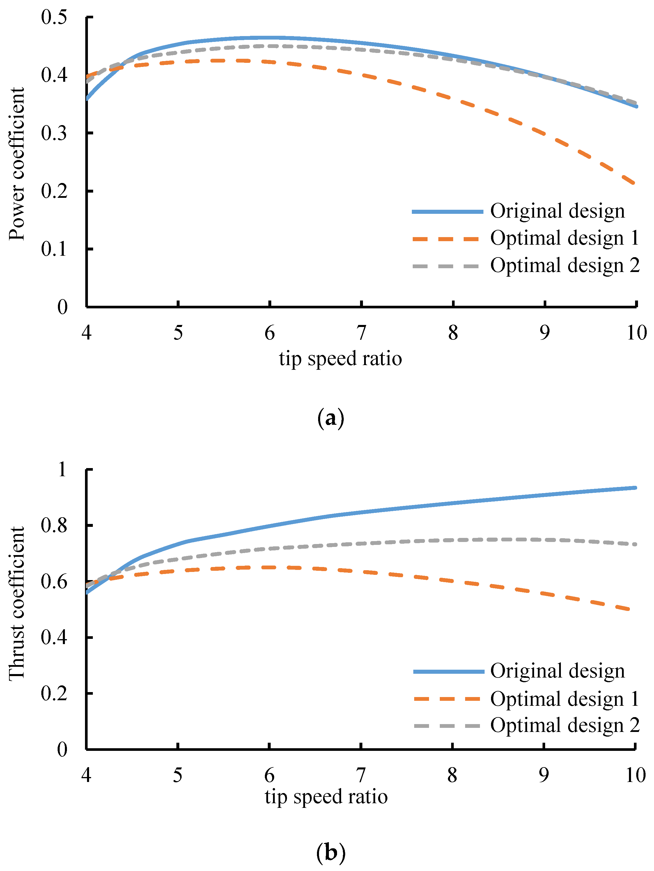
The blade designs presented in
Figure 12 were verified in GH-Bladed [
21]. The predicted power coefficient
CP and thrust coefficient
CT at the rated tip speed ratio are presented in
Figure 13.
Table 4 gives the corresponding fatigue life predicted by the equivalent S–N curve model. As can be seen, a small reduction in power coefficient leads to a large reduction in thrust coefficient and a much larger growth in fatigue life through the proposed improved blade design. In fact, it is an optimized compromise between efficiency and lifetime. Therefore, the solution points generated in
Figure 11 could provide an effective reference for TCT blade developers once the expected power efficiency and work life are clear.
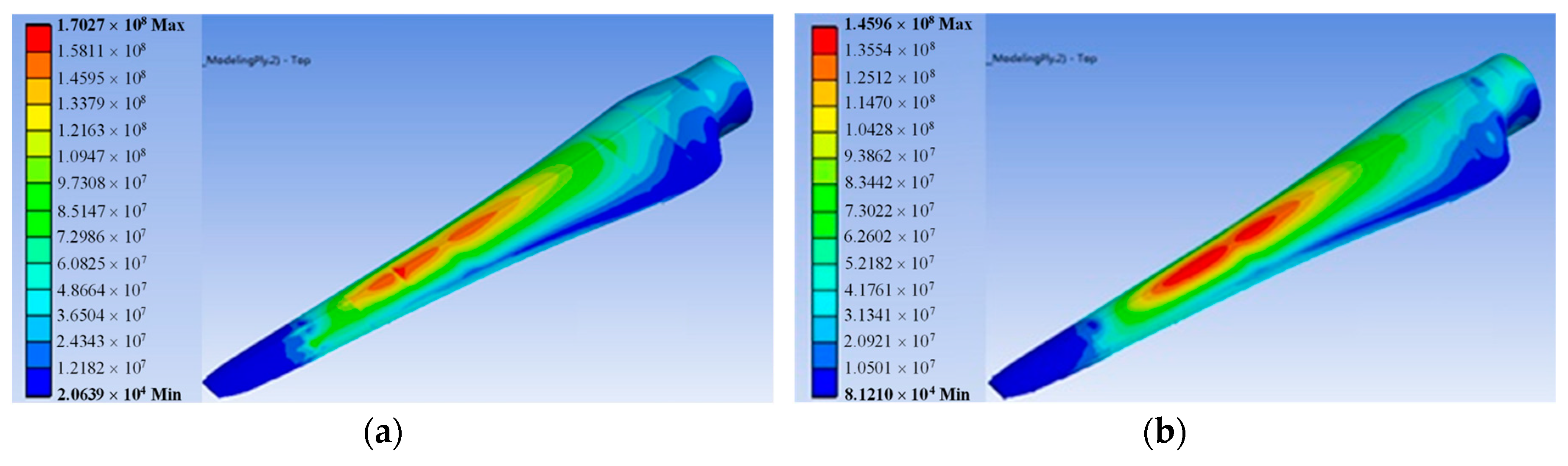
For a further evaluation, an FEA simulation of Optimal design 2 was carried out in combination with the layer method presented in [
22], as shown in
Figure 14. The nominal load under extreme conditions was imposed. A comparison of the FEA simulation results and the optimization effects is given in
Table 5, demonstrating that the proposed blade design method has a significant optimization effect on both the hydrodynamics and structure.
In the above research, a BEM-based model is employed in both the blade optimization design and the simulation of performance coefficients in GH-Bladed. The structural parameters of this model mainly include chord length, twist angle, thickness, and lift/drag curves. However, the BEM-based model is almost ideal with the assumptions of infinitesimal blade element, no medium viscidity, no blade radial flow, and no radial interaction between the elements. Hence, the resultant characteristics of blade would keep a distance from the reality. In the ANSYS software, the CFD model depends upon the solution of the Navier-Stokes equations, representing the conservation of mass and momentum [
23]. The water viscidity, blade radial flow, and the flow field features near the hub are all taken into consideration, that the model has 3D effects. This would increase the accuracy of the hydrodynamics and structural stress estimation. Therefore, the next design work will take into account CFD models with higher fidelity, to improve the optimization effect.
6. Conclusions
With the aim of enhancing the blade reliability of TCTs without efficiency loss, this article details an improved blade design method based on the multi-objective genetic algorithm. This optimization was carried out on a 4.4 m length blade of a 120 kW TCT. An equivalent S–N curve model and a simplified load spectrum were proposed to provide a convenient estimation of the blade fatigue life. Simulations of the comprehensive performance of the blade were conducted using both GH-bladed and ANSYS. The results show that the hydrodynamics, structure, and lifetime of the blade were all greatly improved, with a small sacrifice in terms of power efficiency.
In addition, the Pareto solution set provides other alternative solutions. Through this improved blade design method, a quick decision on blade solutions between lifetime and power output could be more easily made. Hence, it could be used to avoid the time-costly iterations and excessive redundancy in traditional blade design and provide more choices for TCT developers by allowing further economic assessments.


