A Dynamic Multi-Swarm Particle Swarm Optimizer for Multi-Objective Optimization of Machining Operations Considering Efficiency and Energy Consumption

Abstract

Facing energy shortage and severe environmental pollution, manufacturing companies need to urgently energy consumption, make rational use of resources and improve economic benefits. This paper formulates a multi-objective optimization model for lathe turning operations which aims to simultaneously minimize energy consumption, machining cost and cutting time. A dynamic multi-swarm particle swarm optimizer (DMS-PSO) is proposed to solve the formulation. A case study is provided to illustrate the effectiveness of the proposed algorithm. The results show that the DMS-PSO approach can ensure good convergence and diversity of the solution set. Additionally, the optimal machining parameters are identified by fuzzy comprehensive evaluation (FCE) and compared with empirical parameters. It is discovered that the optimal parameters obtained from the proposed algorithm outperform the empirical parameters in all three objectives. The research findings shed new light on energy conservation of machining operations.

1. Introduction

With the soaring demand of energy and the worsening of the environment, modern manufacturing enterprises are faced with new challenges to improve energy efficiency and reduce pollution emissions [1,2,3]. As a result, they have adopted various measures with respect to equipment, technology, materials and other aspects to achieve the purpose of energy conservation, emission reduction, and green manufacturing [4,5,6]. Machine tools are the basic equipment for production and the leading energy consumer in the manufacturing industry [7,8,9,10]. Globally, machining operations consume about 75% of the energy used in manufacturing, but the energy efficiency of the machining systems is below 30% [11]. The enormous energy consumption of machine tools, coupled with their poor energy efficiency, has intensified the concerns of environmental pollution and carbon emissions. To address these concerns, it is imperative to reduce the energy consumption of machine tools for the modern manufacturing industry. The reduction of energy consumption will in turn improve the efficiency of manufacturing enterprises, reduce the production cost, alleviate environmental pollution, and move towards greener and more sustainable manufacturing [12].

It is well known that the machining parameters directly affect product quality, machining cost, production efficiency and energy consumption. Therefore, the optimization of machining parameters has become a key research objective for both industry and academia [13]. For brevity, the representative works in the literature are cited in the following. Arriaza et al. [14] relied on multiple response optimization to analyze the relationship between feed rate and energy consumption in rough machining, and considered feed rate the key to balancing energy and time. Öztürk et al. [15] adopted a Taguchi L9 design and compiled a multi-parameter test table (including tool diameter, cutting depth, cutting speed and feed rate) to minimize the surface roughness and energy consumption of a machining center. The results revealed that the specific energy consumption (SEC) was significantly affected by the maximum cutting depth. Additionally, Hu et al. [16] modelled the machining optimization problem in terms of sequence-related machining time, deviation, and energy consumption, and introduced a multi-objective feature sequencing model that makes a trade-off among the three objectives. Jang et al. [17] considered four machining parameters in the cutting energy model, and the particle swarm optimization approach was adopted to obtain the cutting condition that minimizes the cutting energy. Based on grey relational analysis and the surface response method, Yan et al. [18] obtained the optimal plane milling parameters under the objectives of minimizing cutting energy consumption and surface roughness.

Meanwhile, Subramanian et al. [19] constructed a mathematical model between cutting parameters and cutting force through milling experiments and multivariate regression, and optimized the cutting parameters using the genetic algorithm (GA). He et al. [20] developed a multi-objective optimization model to optimize the energy consumption, cutting force and cutting time of a milling machine, and explored the effects of three solution algorithms (i.e., vector evaluated genetic algorithm, non-dominated sorting genetic algorithm, and multi-objective evolutionary algorithm) on the Pareto frontier. D’Addona and Teti [21] created a multi-objective optimization model for turning operations that considers machining cost, cutting time and machining quality, and proposed a GA-based algorithm to solve the model. To minimize the energy consumption in machining, Velchev et al. [22] formulated an optimization model for process parameters, investigated the impact of lathe cutting parameters (e.g., feed rate and cutting depth) on energy consumption, and concluded that the energy consumption is negatively correlated with feed rate and cutting speed.

Similarly, Xu et al. [23] investigated the cutter path optimization problem and its influencing factors, introduced a cutter path optimization model for maximum machining efficiency and minimum energy consumption, and developed an adaptive simulated annealing genetic algorithm to obtain the optimal cutter path. Based on the design of experiment (DOE) approach, Camposeco-Negrete [24] investigated the effects of depth of cut, feed rate, and cutting speed on machining energy consumption and surface roughness in turning an aluminum alloy. It was claimed that the effect of feed rate is most significant in minimizing the power consumption and surface roughness. To simplify the computation of traditional empirical formula and reduce energy consumption, Kant and Sangwan [25] modelled energy consumption of computer numerical control (CNC) machine tools based on backpropagation neural network (BPNN), and optimized the cutting parameters by the GA. In addition, Shi et al. [26] created an improved energy consumption model for normal vertical milling based on cutting force. The model was applied to study the energy efficiency of normal vertical milling, and thus reveal the relationship between energy consumption and various cutting parameters. To optimize the machining parameters of milling operations, Li et al. [27] developed an optimization model with two objectives, namely, maximizing the energy efficiency and minimizing the production time. A Tabu-search heuristic algorithm was proposed to solve the model. It was found that the depth and width of the cut are the two most influential factors.

Nevertheless, the majority of existing studies on energy consumption of machine tools focus on a single objective, namely, reducing energy consumption or improving energy efficiency [28]. For the limited studies that address the multi-objective issues [29], the algorithms developed to find the optimal solution are usually not flexible. Some studies use the weighting method to transform multiple subjects into a single-subject problem [30]. Nevertheless, this method is often too subjective, and the selection of weights depends on personal experience, which is difficult to determine reasonably. As a result, the results often cannot meet the actual needs. Because optimization objectives are often in conflict with each other for multi-objective optimization problems (MOPs), there could be no single solution that optimizes all objectives simultaneously. More studies have adopted optimization algorithms to obtain the Pareto optimal set instead of a single solution to solve MOPs in recent years [31,32]. The purpose of these multi-objective optimization algorithms is to obtain a set of representative Pareto optimal solutions, and to make the distribution of these Pareto optimal solutions on the target space Pareto Front (PF) as good as possible in terms of approximation, width and uniformity. These optimization algorithms include multi-objective evolutionary algorithm, multi-objective particle swarm optimization (PSO), ant colony optimization, artificial neural network optimization and so on. In particular, PSO features a simple structure and fast convergence speed, and it has been successfully applied to solve single-objective and multi-objective optimization problems [33]. However, PSO often suffers from the loss of population diversity due to its fast convergence rate, and then falls into the local optimal solution, failing to achieve satisfactory results [34].

To overcome these challenges, this paper proposes a multi-objective optimization model for minimizing energy consumption, machining cost, and time in turning operations. A dynamic multi-swarm particle swarm optimizer (DMS-PSO) is conceptualized to converge to a set of diverse solutions, such as selecting suitable process parameters for specific machining requirements and multiple objectives. The DMS-PSO approach divides the swarm into several sub-swarms, and regroups the sub-swarms frequently to exchange information. In the DMS-PSO, the neighborhood topology is adopted, which is random and may dynamically change. The neighborhood topology is suitable for solving complex multi-modal problems and to ensure the diversity of solutions [35]. Please note that in the literature, the general concept of DMS-PSO has been studied to improve the ability of PSO to jump out of the local optimal solution [36,37]. For instance, Chen et al. [38] proposed a novel method to merge the differential evolution operator into each sub-swarm of the DMS-PSO so as to improve the performance of PSO. Meanwhile, DMS-PSO has started to find applications in real-world scenarios. For instance, Xia et al. [39] developed a multiple-swarm framework in combination with the dynamic sub-swarm number strategy. The approach was found to be effective in multiple real-world applications such as in the design of a gear train. Chen et al. [40] applied DMS-PSO to develop optimal strategies for two-variable energy management and gear-shifting in hybrid electric vehicles. It was verified that the DMS-PSO approach generates superior performance compared with the traditional method. On the other hand, the concept of DMS-PSO has rarely (if ever) been applied to optimizing machining energy and efficiency, to the best of our knowledge.

2. Multi-Objective Optimization Model for Machining

Lathe turning is an important machining operation. The market size of CNC lathe had already reached 25.01 billion USD in 2018, and is expected to grow to 40.22 billion USD by 2026 [41]. Additionally, the tool–material interaction in lathe turning represents the fundamentals of material removal for other more complex machining operations such as milling and grinding. As such, lathe turning is adopted as the research problem in this paper. In actual machining, the selection of cutting parameters for CNC machine tools is affected by various factors. For turning operation, the three key process parameters are cutting speed v_c, depth of cut a_p, and feed rate f [42,43]. The specific energy consumption (SEC) and the cutting time of machining are mainly determined by these three process parameters. Other factors such as work material, tool material, tool nose radius, and rake angles will also affect the turning operation and the SEC value, but they are fixed for simplicity in this study. Additionally, note that for a more complex machining process such as milling, additional process parameters such as width of cut need to be considered.

2.1. Energy Consumption

The plastic deformation in the cutting layer of the workpiece is under the combined effects of the following factors and their interactions: cutting force, cutting heat, cutting temperature, cutter angle, and workpiece material. Among them, the cutting force, F_c (N), determines the heat generation, and affects cutter abrasion and quality of the machined surface [44]. In many cases, the complex relationship among the influencing factors can be generally described by an empirical exponential formula [45,46],

$$F_c=C_{Fc}{a}_p^{x_{Fc}}{f}^{y_{Fc}}{v}_c^{z_{Fc}}{K}_{F_c}$$

(1)

where v_c (mm/s), a_p (mm) and f (mm/min) are cutting speed, depth of cut and feed rate, respectively; C_FC is a coefficient determined by workpiece material and cutting condition; x_FC, y_FC and z_FC are exponential constants; K_FC is a correction coefficient.

Based on Equation (1), the cutting power P_c (N·m/s) can be estimated,

$$P_c=\frac{F_c{v}_c}{1000}$$

(2)

In machining, the excess material is removed from the workpiece through the relative motion between the workpiece and the cutter. The machining efficiency can be improved by increasing the material removal rate per unit time and reducing the energy consumption [47]. Hence, SEC, i.e., the ratio of the total energy consumption E to the material removal volume MRV (mm³), is selected as the evaluation index for energy consumption of machining. MRV and SEC can be respectively defined as:

$$MRV={\displaystyle {\int }_0^{T_C}MRR\cdot dt}=\frac{v_c\cdot f\cdot a_p\cdot T_c}{N}$$

(3)

$$SEC=\frac{E}{MRV}=\frac{P_c{T}_c}{MRV}$$

(4)

where MRR is the material removal rate, N is the spindle RPM, and T_c is the cutting time.

2.2. Machining Cost

For a manufacturer, the following costs may be incurred: labor cost, transport cost, inventory cost, depreciation cost of the machine tool, electric energy cost, and cutter depletion cost. Among them, some costs (e.g., transport cost) are not directly related to machining operations. Therefore, this paper mainly considers the depreciation cost of the machine C_M, the cutter depletion cost C_T, the electrical energy cost C_E, and the labor cost C_O.

(1) Depreciation cost C_M

In machining, the depreciation cost of the machine C_M ($/hour) is the product of the cutting time Tc (in seconds) of the workpiece and the depreciation rate R ($/hour) of the machine:

$$C_M=\frac{R\cdot T_c}{3600}$$

(5)

(2) Cutter depletion cost C_T

The depletion of cutters, C_T, is the ratio of the unit price, UP, to the service life, T_l, of the cutter:

$$C_T=\frac{UP\cdot T_c}{T_l}$$

(6)

The tool life T_l of the cutter is related to the parameters of cutting speed v_c, feed rate f, and depth of cut a_p. In many cases, the influence of depth of cut is the least, the influence of feed rate is larger than that of depth of cut, and the cutting speed has the greatest effect on tool life. T_l can be computed by:

$$T_l={\left(K_T\frac{C_T}{v_c{a}_p^{x_T}{f}^{y_T}}\right)}^{1/m}$$

(7)

where m, x_T, y_T, C_T and K_T are the coefficients related to the service life of workpiece and cutters.

(3) Energy cost C_E

For a machine tool, the electric energy cost C_E can be measured by the industrial electricity charge of the machining process:

$$C_E=ER\cdot E$$

(8)

where ER is the industrial electricity rate.

(4) Labor cost C_O

The labor cost C_O is the salary paid to operators, which can be estimated based on the cutting time:

$$C_O=\frac{HL\cdot T_C}{3600}$$

(9)

where HL is the hourly rate of an operator.

To sum up, the machining cost C_t can be calculated:

$$C_t=C_M+C_T+C_E+C_O$$

(10)

2.3. Cutting Time

The total machining time can be broken down into standby time, idling time, tool change time and cutting time. However, since this research only tackles the actual cutting process, other machining time components are not considered. The cutting time Tc can be computed in terms of feed rate f and cutting length L,

$$T_c=\frac{L}{f}$$

(11)

2.4. Constraints

The cutting parameters of machine tools must satisfy various constraints on machine tool performance and machining conditions, including cutting speed, surface roughness, machine tool power and the maximum cutting force.

(1) Machining parameters

For a machine tool, the three machining parameters (i.e., cutting speed, feed rate, and depth of cut) must fall into an interval for any machining condition,

$$v_{\min }\le v\le v_{\max }$$

(12)

$$f_{\min }\le f\le f_{\max }$$

(13)

$$a_p{}_{\min }\le a_p\le a_p{}_{\max }$$

(14)

(2) Power of machine tool

In real-world conditions, the maximum cutting power is limited by the power of the spindle motor in the machine tool. Hence, the power of machine tool should not exceed the spindle motor power P_{c max}:

$$P_c=\frac{C_{Fc}{a}_p^{x_{Fc}}{f}^{y_{Fc}}{v}_c^{z_{Fc}+1}{K}_{F_c}}{1000{\eta }_m}\le P_{c\max }$$

(15)

where η_m is the transmission efficiency of the machine tool.

(3) Cutting force [45]

Generally, the force of the main cutter is taken as the cutting force of the entire machine tool. The magnitude of the force must be within the scope of the maximum cutting force provided by the machine tool:

$$F_c=C_{Fc}{a}_p^{x_{Fc}}{f}^{y_{Fc}}{v}_c^{z_{Fc}}{K}_{F_c}\le F_{\max }$$

(16)

(4) Surface roughness [48]

In machining, the surface roughness of the workpiece is related to the process requirements, workpiece material and the required workpiece performance. Here, the surface roughness should satisfy the following constraint,

$$R_a=r_c-\sqrt{r_c-{\left(\frac{f}{2N}\right)}^2}\le R_{\max }$$

(17)

where r_c is the corner radius of the cutter.

In summary, the multi-objective optimization model of the machining parameters for machine tools can be established as:

$$\min \{\begin{array}{c}\mathrm{SEC}=\frac{\mathrm{E}}{\mathrm{MRV}}\\ {\mathrm{T}}_{\mathrm{c}}=\frac{\mathrm{L}}{\mathrm{f}}\\ {\mathrm{C}}_{\mathrm{t}}{=\mathrm{C}}_{\mathrm{M}}{+\mathrm{C}}_{\mathrm{T}}{+\mathrm{C}}_{\mathrm{E}}{+\mathrm{C}}_{\mathrm{o}}\end{array}$$

$$\mathrm{s.t.}\{\begin{array}{c}{\mathrm{v}}_{\min }\le \mathrm{v}\le {\mathrm{v}}_{\max }\\ {\mathrm{f}}_{\min }\le \mathrm{f}\le {\mathrm{f}}_{\max }\\ {\mathrm{a}}_{\mathrm{p}\min }\le {\mathrm{a}}_{\mathrm{p}}\le {\mathrm{a}}_{\mathrm{p}\max }\\ {\mathrm{P}}_{\mathrm{c}}=\frac{{\mathrm{C}}_{{\mathrm{F}}_{\mathrm{c}}}{\mathrm{a}}_{\mathrm{p}}^{{\mathrm{x}}_{{\mathrm{F}}_{\mathrm{c}}}}{\mathrm{f}}^{{\mathrm{y}}_{{\mathrm{F}}_{\mathrm{c}}}}{\mathrm{v}}_{\mathrm{c}}^{{\mathrm{z}}_{{\mathrm{F}}_{\mathrm{c}}}+1}{\mathrm{K}}_{{\mathrm{F}}_{\mathrm{c}}}}{{1000\mathsf{\eta }}_{\mathrm{m}}}\le {\mathrm{P}}_{\mathrm{c}\max }\\ {\mathrm{F}}_{\mathrm{c}}{=\mathrm{C}}_{{\mathrm{F}}_{\mathrm{c}}}{\mathrm{a}}_{\mathrm{p}}^{{\mathrm{x}}_{{\mathrm{F}}_{\mathrm{c}}}}{\mathrm{f}}^{{\mathrm{y}}_{{\mathrm{F}}_{\mathrm{c}}}}{\mathrm{v}}_{\mathrm{c}}^{{\mathrm{z}}_{{\mathrm{F}}_{\mathrm{c}}}}{\mathrm{K}}_{{\mathrm{F}}_{\mathrm{c}}}\le {\mathrm{F}}_{\max }\\ {\mathrm{R}}_{\mathrm{a}}{=\mathrm{r}}_{\mathrm{c}}-\sqrt{{\mathrm{r}}_{\mathrm{c}}-{\left(\frac{\mathrm{f}}{2\mathrm{N}}\right)}^2}\le {\mathrm{R}}_{\max }\end{array}$$

3. Solution Approach

3.1. Concept of DMS-PSO Algorithm

The particle swarm optimization (PSO) [49,50] is an evolutionary algorithm mimicking the behavior of individuals in a swarm to maximize the survival of the species. With simple concepts and few adjustable parameters, the PSO is easy to program, implement, and combine with other algorithms. More importantly, the algorithm can adapt to various conditions and converge to the optimal solution rapidly. Considering these advantages, this paper selects the PSO to solve our multi-objective optimization model.

The PSO is an iteration-based optimization algorithm. In each iteration, every particle determines its velocity and position for the next step according to its current position and velocity, its best-known position and velocity and the global best-known position and velocity. The position and velocity update formulas are as follows:

$$\{\begin{array}{c}{\mathit{v}}_{\mathit{id}}^{(\mathit{k}+1)}=\mathsf{\omega }·{\mathit{v}}_{\mathit{id}}^{\left(\mathit{k}\right)}{+\mathit{c}}_1·{\mathit{r}}_1·\left({\mathit{p}}_{\mathit{id}}^{\left(\mathit{k}\right)}{-\mathit{x}}_{\mathit{id}}^{\left(\mathit{k}\right)}\right){+\mathit{c}}_2·{\mathit{r}}_{2\mathit{x}}·\left({\mathit{g}}_{\mathit{id}}^{\left(\mathit{k}\right)}{-\mathit{x}}_{\mathit{id}}^{\left(\mathit{k}\right)}\right)\\ {\mathit{x}}_{\mathit{id}}^{(\mathit{k}+1)}{=\mathit{x}}_{\mathit{id}}^{\left(\mathit{k}\right)}{+\mathit{v}}_{\mathit{id}}^{(\mathit{k}+1)}\end{array}$$

(18)

Any new particle velocity produced by the neighborhood function must fall below the maximum velocity:

$$\left|{\mathit{v}}_{\mathit{id}}^{\left(\mathit{k}\right)}\right|\le {\mathit{V}}_{\mathit{max}}$$

(19)

The selection function of the PSO can be defined as:

$$D\left(Ø{(\mathit{x}}_{\mathit{i}}^{\left(\mathit{k}\right)}{),\mathit{p}}_{\mathit{id}}^{\left(\mathit{k}\right)}\right)=\{\begin{array}{c}Ø{(\mathit{x}}_{\mathit{i}}^{\left(\mathit{k}\right)}\left)\mathit{f}\right(Ø{(\mathit{x}}_{\mathit{i}}^{\left(\mathit{k}\right)}\left)\right)\le {\mathit{f}(\mathit{p}}_{\mathit{id}}^{\left(\mathit{k}\right)})\\ {\mathit{p}}_{\mathit{id}}^{\left(\mathit{k}\right)}\mathit{f}(Ø{(\mathit{x}}_{\mathit{i}}^{\left(\mathit{k}\right)}{\left)\right)\mathit{f}(\mathit{p}}_{\mathit{id}}^{\left(\mathit{k}\right)})\end{array}$$

(20)

where $p_{\mathrm{id}}^{(k)}$ and $g_{\mathrm{id}}^{(k)}$ should be selected by the following criteria:

$${\mathit{p}}_{\mathit{id}}^{\left(\mathit{k}\right)}\in \left\{{\mathit{x}}_{1\mathit{d}}^{\left(\mathit{k}\right)}{,\mathit{x}}_{2\mathit{d}}^{\left(\mathit{k}\right)},\cdots {,\mathit{x}}_{\mathit{Nd}}^{\left(\mathit{k}\right)}{\left|\mathit{f}\right(\mathit{x}}_{\mathit{id}}^{\left(\mathit{k}\right)})\right\}=\mathit{min}\left\{\mathit{f}\left({\mathit{x}}_{1\mathit{d}}^{\left(\mathit{k}\right)}\right),\mathit{f}\left({\mathit{x}}_{2\mathit{d}}^{\left(\mathit{k}\right)}\right),\cdots ,\mathit{f}\left({\mathit{x}}_{\mathit{Nd}}^{\left(\mathit{k}\right)}\right)\right\}$$

(21)

$${\mathit{g}}_{\mathit{id}}^{\left(\mathit{k}\right)}\in \left\{{\mathit{g}}_{1\mathit{d}}^{\left(\mathit{k}\right)}{,\mathit{g}}_{2\mathit{d}}^{\left(\mathit{k}\right)},\cdots {,\mathit{g}}_{\mathit{Nd}}^{\left(\mathit{k}\right)}{\left|\mathit{f}\right(\mathit{p}}_{\mathit{id}}^{\left(\mathit{k}\right)})\right\}=\mathit{min}\left\{\mathit{f}\left({\mathit{g}}_{1\mathit{d}}^{\left(\mathit{k}\right)}\right),\mathit{f}\left({\mathit{g}}_{2\mathit{d}}^{\left(\mathit{k}\right)}\right),\cdots ,\mathit{f}\left({\mathit{g}}_{\mathit{Nd}}^{\left(\mathit{k}\right)}\right)\right\}$$

(22)

The meanings of symbols in the above equations are explained in

Table 1. Symbols for PSO parameters

$\mathsf{\omega }.$	Inertia Weight	${\mathbf{V}}_{\mathbf{max}}$	Maximum Velocity
$\mathrm{g}$	Iteration cycle	$c_1$ and $c_2$	Learning factors
${\mathrm{x}}_{\mathrm{i}}^{\left(\mathrm{k}\right)}$	Current position	r1r2	A random number in interval [0,1]
${\mathrm{v}}_{\mathrm{i}}^{\left(\mathrm{k}\right)}$	Velocity	N	Quantity of swarm
${\mathrm{p}}_{\mathrm{id}}^{\left(\mathrm{k}\right)}$	Individual best-known position	d	Dimension of search space
${\mathrm{g}}_{\mathrm{id}}^{\left(\mathrm{k}\right)}$	Global best-known position	$\mathrm{f}(·)$	Fitness function

below.

Because of the fast convergence, the PSO is very likely to undermine swarm diversity and fall into the local optimum trap [51]. To solve these problems, this paper introduces the DMS strategy to the PSO, which divides the swarm into several sub-swarms by certain rules. The sub-swarms are reconstructed through the search process, such that their particles can change dynamically. Thus, the multiple sub-swarms can exchange information, in the meantime of parallel search and co-evolution.

Suppose the original swarm has nine particles and is divided into three sub-swarms. In the DMS-PSO, the sub-swarms are reconstructed by the following rules: Each sub-swarm searches for better solutions with their particles. During the search, the sub-swarm may converge to the local optimum solutions. Next, the nine particles were regrouped into three new sub-swarms every other R iterations. The new sub-swarms will start to search for the optimal solution again. The above process is repeated until the termination condition is satisfied [37,52]. By the reconstruction strategy, the particles from different sub-swarms are repeatedly regrouped into new sub-swarms. Thus, the search space of each sub-swarm is expanded, enabling it to find the better solution. This strategy also helps to diversify the particles. Compared with the traditional swarm structure, the new swarm structure has greater degree of freedom and performs better in complex multi-modal problems.

3.2. Multi-Objective Consideration

Multi-objective optimization problems have essential differences with single objective optimization problems [53] in that multi-objective optimization needs to coordinate or make a trade-off between the multiple objectives under the specified constraints, aiming to achieve the best overall performance. Therefore, the key to solve a constrained multi-objective optimization problem lies in the processing of the objectives and constraints.

In the multi-objective optimization model, energy consumption, machining cost and cutting time place restriction against each other. The three objectives differ greatly in meaning and dimensions, making it difficult to compare or weigh them directly. To provide accurate information for decision-makers, this paper adopts the Pareto optimal set to solve the multi-objective optimization problem. The separation index method, which does not directly discard the non-feasible particles, is selected to process the multiple objectives and constraints, and ensure the solution diversity and convergence. By this method, the total deviation of each non-feasible particle from all constraints is considered the distance measure of the feasible region. Then, all particle positions are ranked by the sum of the target fitness and the deviation. To reflect the optimization difficulties of each particle under different constraints, the deviation Φ_i of a particle from a constraint can be defined as [54],

$${Ø}_{\mathit{i}}=\frac{{{\displaystyle \sum }}_{\mathit{j}-1}^{\mathit{N}}{\mathit{G}}_{\mathit{i}}\left({\mathit{x}}_{\mathit{j}}\right)}{{{\displaystyle \sum }}_{\mathit{j}-1}^{\mathit{N}}{{\displaystyle \sum }}_{\mathit{j}-1}^{\mathit{N}}{\mathit{G}}_i\left({\mathit{x}}_{\mathit{j}}\right)},\mathit{i}=1,2,\cdots ,\mathit{n}$$

(23)

$${\mathit{G}}_{\mathit{i}}\left(\mathit{x}\right)=\{\begin{array}{c}\mathit{max}\left\{{\mathit{g}}_{\mathit{i}}\left(\mathit{x}\right),0\right\},\mathit{i}=1,2,\cdots ,\mathit{p}\\ \mathit{max}\left\{\left|{\mathit{h}}_{\mathit{i}}\left(\mathit{x}\right)\right|-\mathsf{\epsilon },0\right\},\mathit{i}=\mathit{p}+1,\mathit{p}+2,\cdots ,\mathit{n}\end{array}$$

(24)

where G_i(x) is the deviation of particle x in the swarm from the i-th constraint; n is the number of constraints; x_j is the j-th particle of the swarm; ε is the tolerance coefficient of the deviation; N is the swarm size.

Then, the fitness of each particle can be defined as:

$$\mathit{F}\left(\mathit{x}\right)=\{\begin{array}{c}{\mathit{f}}_{\mathit{i}}\left(\mathit{x}\right)\mathit{Feasible}\mathit{particle}\\ {\displaystyle {\displaystyle \sum }_{\mathit{j}-1}^{\mathit{N}}}{Ø}_{\mathit{j}}\left(\mathit{x}\right) \mathit{Non}-\mathit{feasible}\mathit{particle}\end{array}$$

(25)

The particles need to select between solutions that both optimize the objectives and satisfy the constraints. Thus, the solution quality is judged by the following criteria rather than fitness alone:

(1)

If both solutions are feasible, the one with the higher fitness should be selected;

(2)

If one solution is feasible and the other is non-feasible, the feasible one should be selected;

(3)

If both solutions are non-feasible, the one with the smaller deviation should be selected.

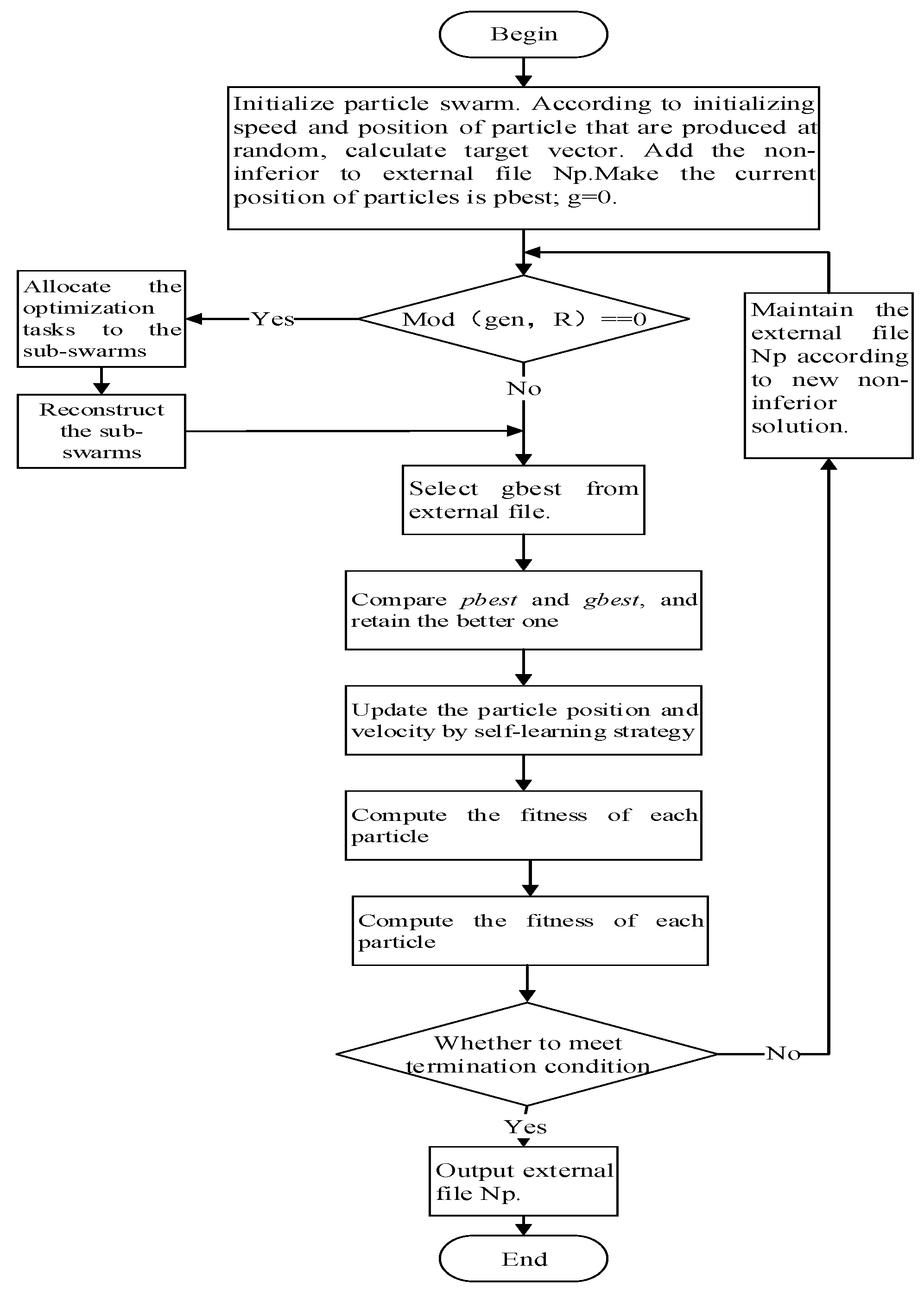
3.3. Procedure of the DMS-PSO Approach

Based on the multi-objective optimization strategy in literature [55], we refine the procedure of the DMS-PSO approach to solve the multi-objective optimization model for machining parameters of machine tools. As shown in Figure 1, the steps of the DMS-PSO are as follows:

Step 1.

Initialize the swarm under the constraints of the model. Determine the initial position and velocity of each particle.

Step 2.

Judge if the swarm reaches the condition for division.

Step 3.

Allocate the optimization tasks to the sub-swarms.

Step 4.

Reconstruct the sub-swarms by the strategy in Section 3.1.

Step 5.

Select the global best-known solution gbest from the external file by tournament selection.

Step 6.

Compare pbest and gbest, and retain the better one.

Step 7.

Update the particle position and velocity by self-learning strategy, while ensuring the flight in the search space.

Step 8.

Compute the fitness of each particle.

Step 9.

Add the new non-inferior solutions to the external file N_p.

Step 10.

Judge if the termination condition is met.

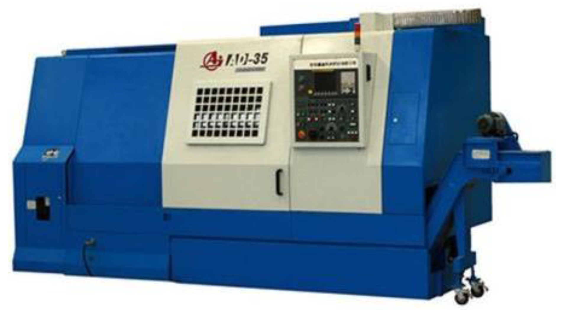
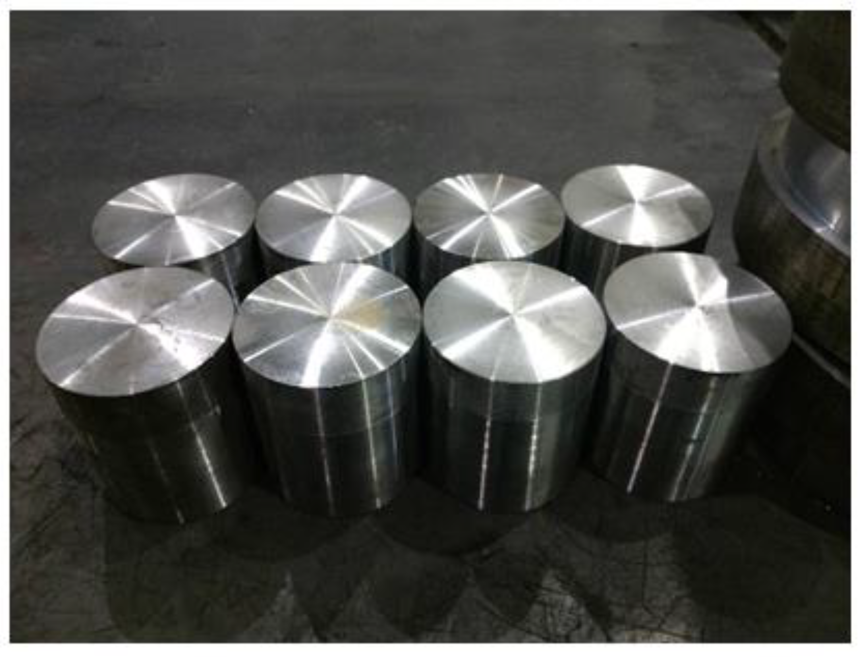
4. Numerical Case

4.1. Machining Scenario

The turning scenario employs an AD-35 CNC lathe, as shown in Figure 2, whose spindle speed range is 25~2500 rpm, peak feed rate is 1260 mm/min, and spindle power is 30 kW. Hard alloy cutters are employed, with the rake angle, clearance angle, cutting edge angle, cutting edge inclination angle and corner radius of 15°, 8°, 75° 6° and 1 mm, respectively. As shown in Figure 3, the Φ 89 workpieces to be machined are made of 40Cr steel. The goal of turning is to semi-finish them to the diameter of Φ86 mm for the length of 70 mm, and the surface roughness Ra should be below 6.3 μm.

In the course of machining, the depreciation cost of the machine tool C_M is 29 $/h, the industrial electricity rate is 0.78 $/kWh, the labor cost is 20 $/h, and the cutter cost is 17 $/each. According to literature, the coefficients related to the service life of cutters m, x_T, y_T and CT are set to 0.2, 0.15, 0.35 and 241, respectively [56].

4.2. Simulation Conditions

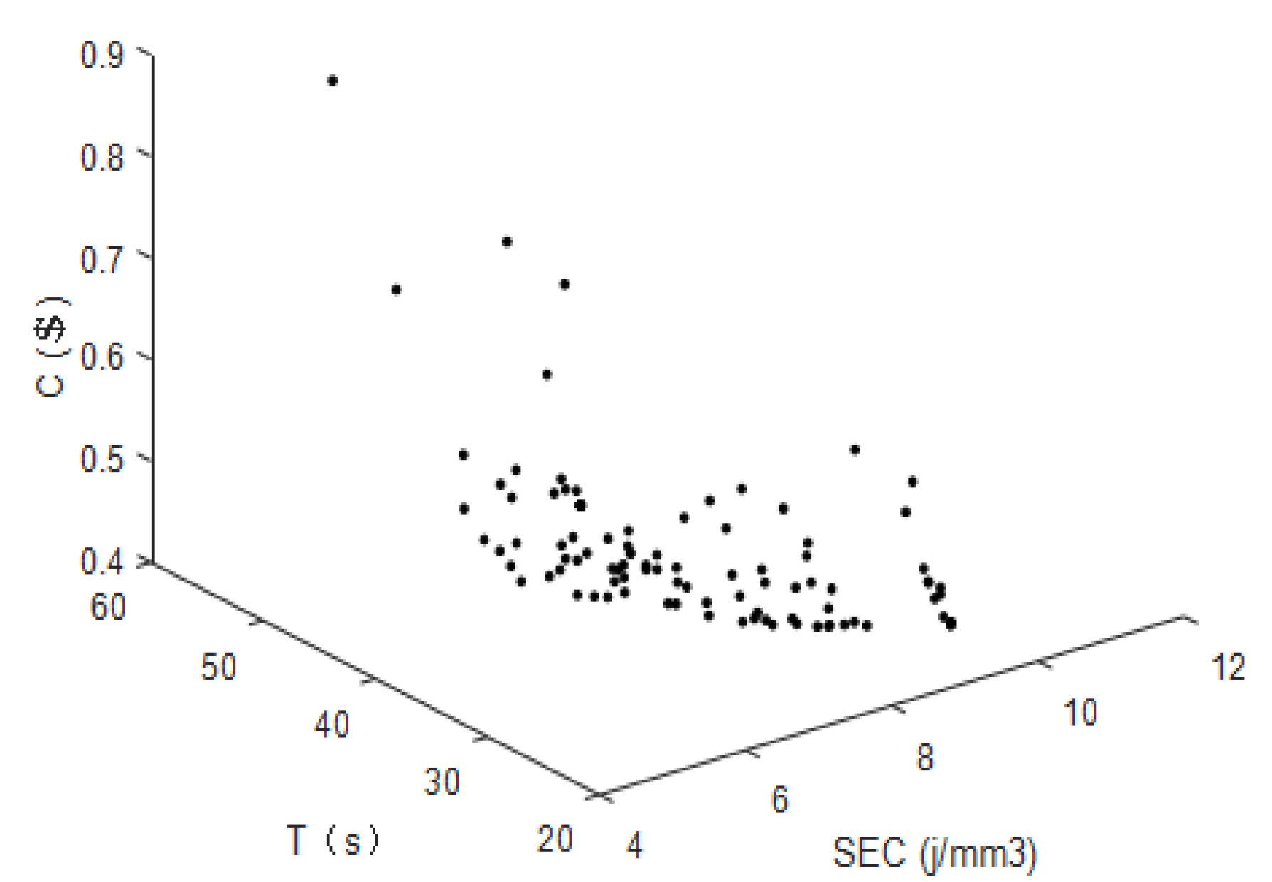
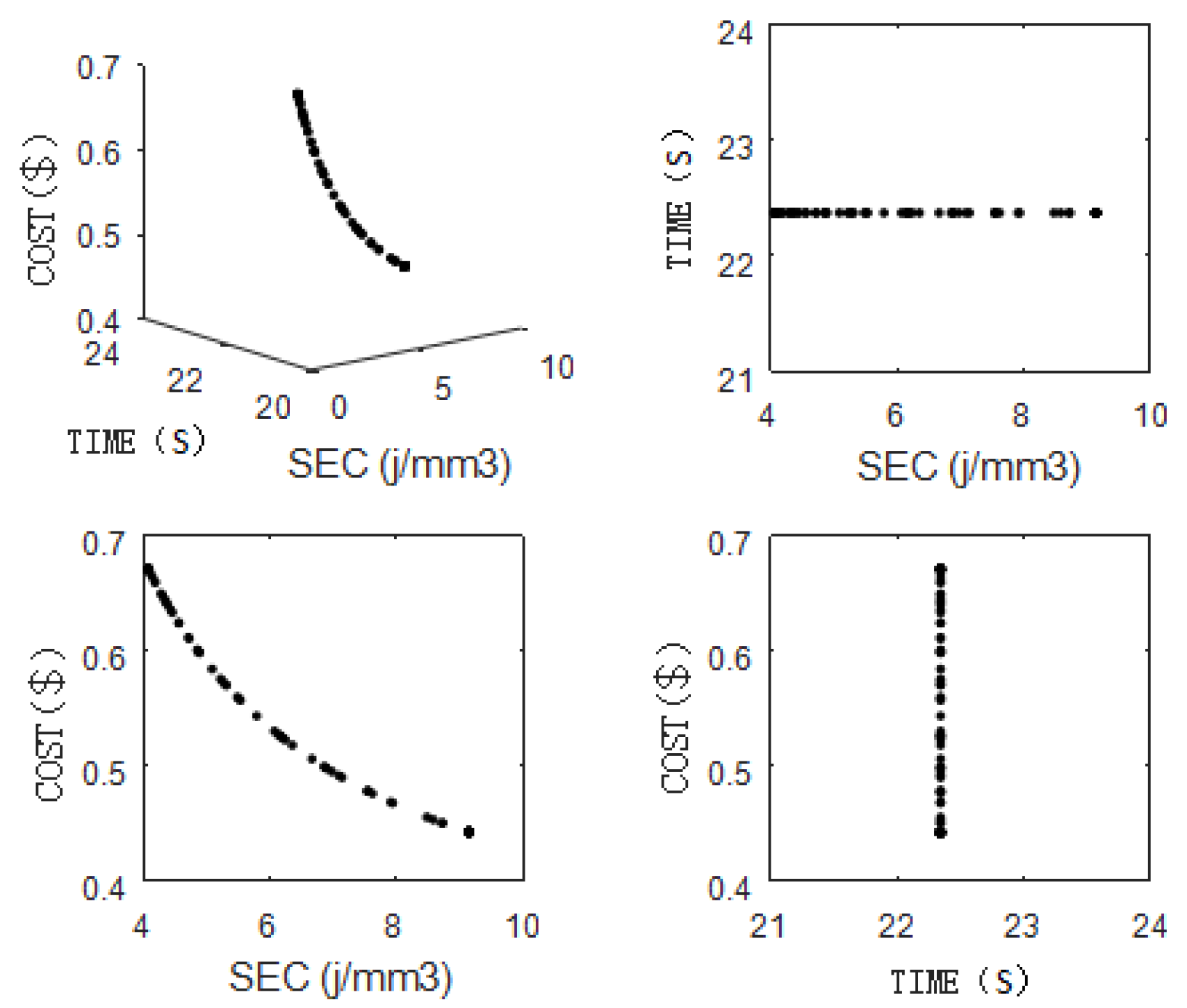
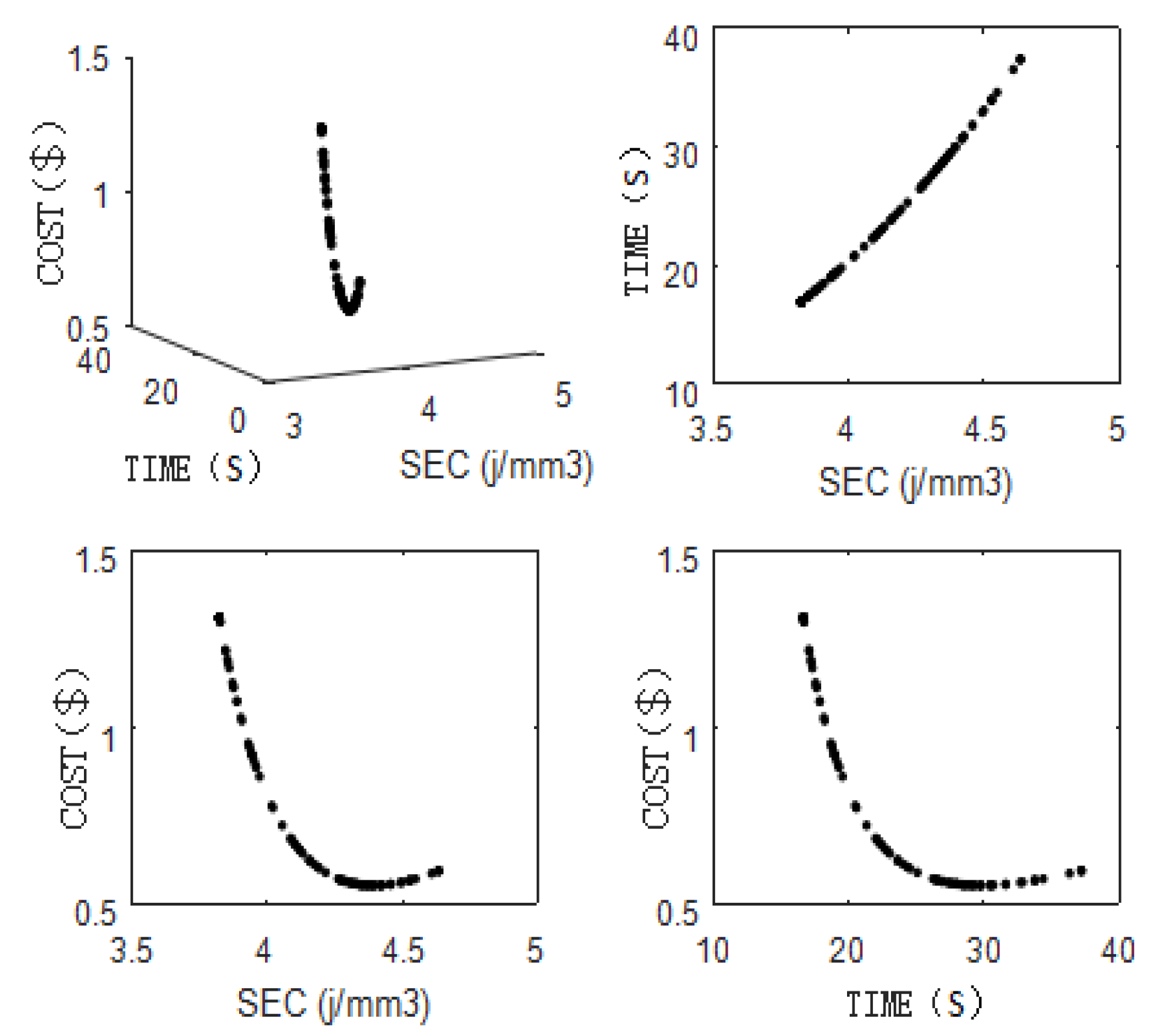
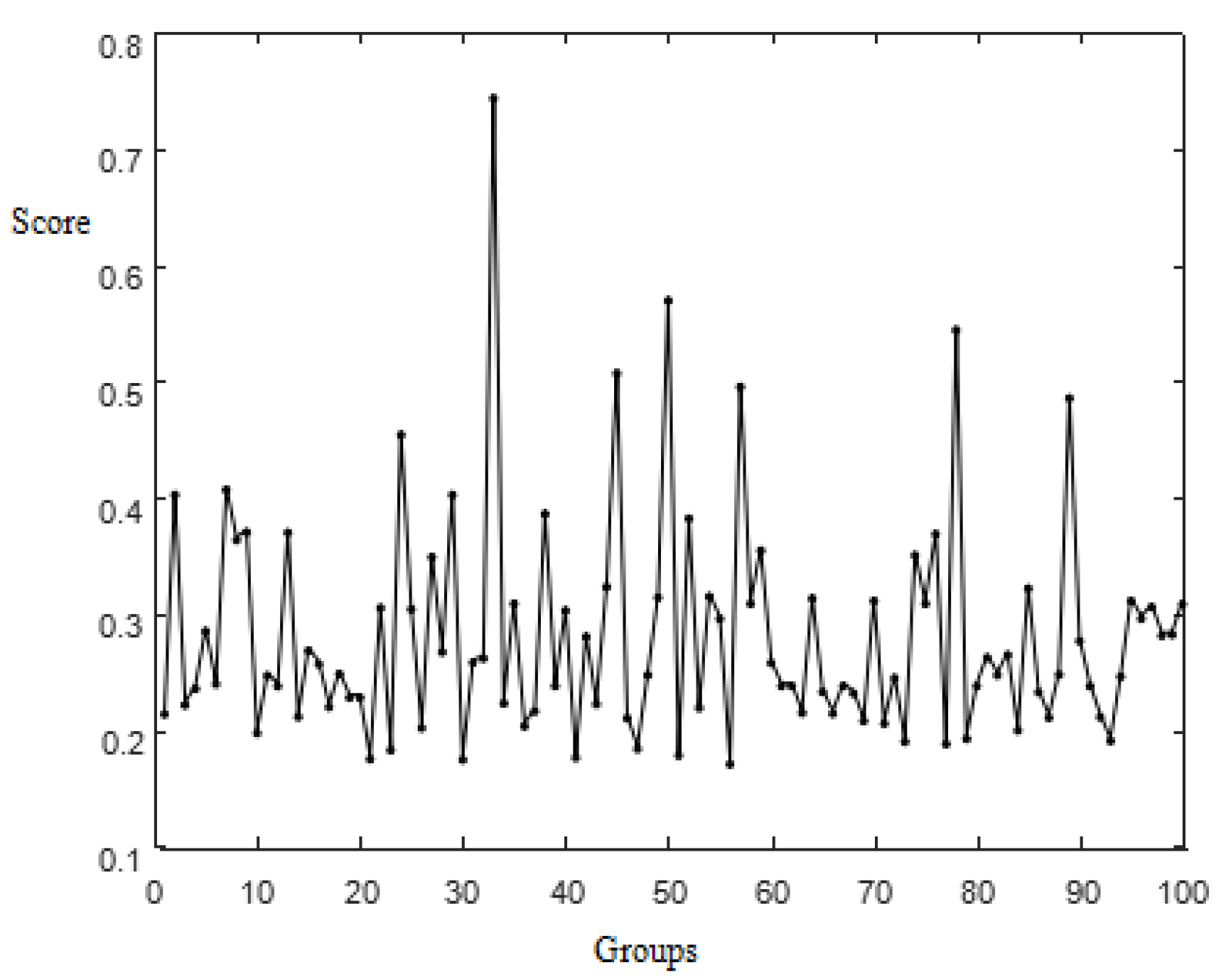
The model is solved by the DMS-PSO approach coded in Matlab 2016b, on a PC (Intel CPU, 2.6GHz, 4GB RAM) running on Windows 10. Based on the existing research related to DMS-PSO [57,58] and the satisfactory results from pilot tests, the number of iterations is set to 1000. To ensure the solution diversity, the recombination interval, self-learning threshold and swarm size are set to 50, 0.5 and 200 respectively based on a pilot test. The parameter settings, simulation results and part of the set of optimal solutions are presented in

Table 2. DMS-PSO parameter settings.

Parameters	Value
Swarm size p	200
Maximum number of iterations g	1000
Inertia weight $\omega$	0.4
Learning factors c1 and c2	2
Capacity of external file $\overline{N}$	100
Reconstruction interval R	50
Self-learning threshold P1	0.5

and

Table 3. Part of the optimal solution set.

Serial Number	vc m/min	f mm/r	ap mm	SEC j/mm3	Tc S	Ct $
1	140.33	0.35	0.92	6.554	23.898	0.492
2	107.39	0.33	0.69	8.490	32.852	0.510
3	150.00	0.35	0.90	6.526	22.357	0.511
4	129.40	0.35	0.84	7.028	25.915	0.474
5	129.19	0.35	0.67	8.078	26.174	0.459
6	119.74	0.35	0.94	6.692	28.006	0.485
7	150.00	0.25	2.00	5.035	31.433	0.726
8	131.22	0.34	0.50	9.619	26.234	0.445
9	122.79	0.35	0.50	9.621	27.311	0.445
10	106.29	0.35	1.92	4.558	31.549	0.547
11	150.00	0.33	1.53	5.006	24.003	0.615
12	109.67	0.35	1.20	5.953	30.577	0.511
13	107.89	0.35	0.65	8.556	31.084	0.485
14	150.00	0.35	1.42	4.998	22.357	0.591
15	140.46	0.30	2.00	4.546	27.586	0.642
16	134.28	0.31	1.37	5.639	28.180	0.562
17	116.05	0.33	2.00	4.554	31.024	0.573
18	147.43	0.35	0.70	7.575	22.746	0.473
19	139.79	0.33	1.33	5.522	25.755	0.556
20	138.66	0.35	0.82	7.011	24.185	0.477
21	128.93	0.35	2.00	4.285	26.307	0.573
22	124.99	0.28	2.00	4.857	33.033	0.627
23	124.89	0.35	1.54	5.025	27.168	0.532
24	106.29	0.35	0.50	9.971	31.604	0.481
25	150.00	0.30	1.19	6.157	26.523	0.589
26	141.23	0.35	1.04	6.068	23.745	0.510
27	128.93	0.35	0.50	9.509	26.009	0.438
28	129.30	0.31	1.19	6.150	28.920	0.538
29	119.04	0.30	0.83	7.961	33.141	0.539
30	113.77	0.35	2.00	4.385	29.475	0.547
$⋮$	…	…	…	…	…	…

and Figure 4, respectively. It can be seen from Figure 4 that the solution set of the DMS-PSO is not clustered in a small area but distributed across a curved surface.

Then, the feed rate, depth of cut and cutting speed are analyzed to disclose their impacts on the three objectives and the convergence of the DMS-PSO. As shown in Table 3, the feed rates are mostly close to the upper limit of 0.35 mm/r. This is because the increase of feed rate can reduce the SEC, the cutting time and the machining cost. In actual production, the feed rate should be rationalized to lower the cost and energy consumption, and improve the machining efficiency. Taking the feed rate of 0.35 mm/r, machining scenarios are developed at the depth of cut of 2 mm or the cutting speed of 150 m/min. The results are displayed in Figure 5 and Figure 6.

As shown in Figure 5 and Figure 6, the Pareto frontier gradually stabilizes with the increase in the number of iterations, and the final solution set obeys a linear distribution, when the depth of cut and cutting speed are taken as the decision variables, respectively. Thus, the Pareto frontiers of the DMS-PSO have good diversity and convergence. In addition, Figure 5 shows that the cutting time has little to do with depth of cut. This seems to be counter intuitive because depth of cut usually significantly affects the machining efficiency—the larger the depth of cut, the shorter the process time to remove the desired amount of material. However, the particular case adopted in this paper is for the semi-finishing process in lathe turning, mainly to ensure that the finishing step has a more uniform machining margin. The semi-finishing turning only needs one pass (or to be cut once), so the cutting time is only related to the workpiece length and the feed rate, but not the depth of cut. Without considering this objective, the greater the depth of cut, the smaller the SEC, and the higher the machining cost. This is attributable to the following factors: with a high depth of cut, the cutters are worn rapidly, pushing up the MRR and energy consumption; but the increment of energy consumption is smaller than that of the MRR. Therefore, the selection of depth of cut directly bears on the machining cost and energy consumption.

From Figure 6, it can be seen that without considering the machining cost, the increase in cutting speed shortens the cutting time and reduces the energy consumption. Without considering the cutting time, the machining cost first declines and then increases, while the SEC reduces with the growth of cutting speed. Without considering the SEC, the machining cost still decreases and then rebounds, while the cutting time is shortened with the increase of cutting speed. The main reason is that while the increasing cutting speed does reduce the cutting time, it intensifies energy consumption and cutter wear.

The above analysis shows that the Pareto frontier obtained by the DMS-PSO boasts good diversity and convergence, providing a suitable way to select the suitable cutting parameters for optimizing multiple objectives in enterprises.

4.3. Discussion

After the optimal solution set is obtained by the DMS-PSO algorithm, one can further comprehensively evaluate the solution set of Pareto from the perspectives of representativeness, systematicness and applicability according to the actual situation of the evaluation system. The methods commonly used for this type of comprehensive evaluation include qualitative method and quantitative methods such as analytic hierarchy process, fuzzy comprehensive evaluation (FCE) and others. In actual production, the equipment, requirements and methods of machining may vary with the types of products and technical levels of operators. Therefore, the weights of the three objectives in machining should be adjusted based on the specific type of products and technical skill of operators. It is difficult to determine or quantify the fuzzy attributes, features and weights of the multi-objective optimization problem. To further evaluate the solution set of Pareto in the turning operations, the fuzzy comprehensive evaluation (FCE) method is introduced in this paper. Based on fuzzy mathematics, the FCE can quantify some fuzzy factors that are unclear in boundaries and difficult to determine or quantify. Firstly, the qualification problem is turned into a quantification problem. Then, the membership of each fuzzy factor is obtained according to the influencing factors, and the quality of that factor is evaluated in a comprehensive manner [59]. The specific steps are as follows:

(1) Determination of evaluation factors

The factor set that influences the selection of Pareto solution set in the multi-objective optimization model of machining parameters is expressed as U.

$$U=\left\{u_1,u_2,\cdots ,u_m\right\}$$

(26)

(2) Establishment of evaluation set

An evaluation set is a set of possible evaluation results made by the evaluator. Let V denote the symbol of the set.

$$V=\left\{v_1,v_2,\cdots ,v_m\right\}$$

(27)

where v_i represents the ith evaluation result and m is the total evaluation result. To select reasonable solutions from the Pareto solution set, four evaluation results will be selected to establish the evaluation set, V = {very important, important, general, not important}.

(3) Judgment matrix construction and weight determination

The single factor evaluation vector is determined by investigation and statistics combined with the research problem. It can be obtained through selecting the membership degree r_ij for the rating v_i.

$$r_i=\left(r_{i1},r_{i2},\cdots ,r_{im}\right)$$

(28)

The total evaluation matrix can be obtained after the comprehensive evaluation of all the factors.

$$\mathbf{R}={(r_{ij})}_{n\times m}=\left[\begin{array}{l}{\mathbf{R}}_1\\ {\mathbf{R}}_2\\ ⋮\\ {\mathbf{R}}_n\end{array}\right]=\left[\begin{array}{l}{r}_{11}{r}_{12}\cdots r_{1m}\\ r_{21}{r}_{22}\cdots r_{2m}\\ ⋮\hspace{1em}⋮\hspace{1em}⋮\hspace{1em}⋮\\ r_{n1}{r}_{n2}\cdots r_{nm}\end{array}\right]$$

(29)

It is not enough to evaluate each solution of the Pareto solution set to obtain the above fuzzy relation matrix. In the actual manufacturing process, evaluation factors have different emphases and functions related to products, technical level of workers, machine tools and equipment. This means that each evaluation index occupies a different proportion in the comprehensive evaluation. As such, a weight distribution set is used, A = (a₁, a₂, …, a_n), where $a_i\ge 0$ and ${\displaystyle \sum a_i}=1$.

(4) Fuzzy synthesis and decision making

There are two kinds of fuzzy synthesis algorithms: the weighted average model and the dominant factor model. Compared with the dominant factor model, the weighted average model has the advantages of making each factor contribute to the evaluation, reflecting and evaluating the whole project objectively, and avoiding the loss of information. Therefore, this paper selects the weighted average fuzzy synthesis algorithm. A fuzzy subset B = (b₁, b₂, …, b_m) that belongs to V is introduced as the decision set, and the evaluation model can be obtained as follows:

$$\mathbf{B}=\mathbf{A}\ast \mathbf{R}=\left(a_1,a_2,\cdots ,a_n\right)\ast \mathbf{R}$$

(30)

If the evaluation result ${{\displaystyle \sum }}^{\hspace{1em}}{b}_i\ne 1$, the fuzzy distribution method is adopted to normalize the evaluation index. Then, the index weights of pareto solution set for different products, processing requirements, machine tools and workers can be obtained.

The importance of energy consumption, machining cost and cutting time for machining depends on many factors such as the equipment condition, products to be produced, technical level of operators, and priority of a company. Thus, the weights of the three objectives could vary with the batches of products. As a result, each type of machine tool has a unique set of weights for the objectives. In light of the actual situation, the weights and judgment matrix are first established, and the optimal combination for the three objectives is then obtained as B = [0.37, 0.21, 0.42] through the FCE. Thereafter, the optimal results are evaluated by the linearly weighted sum method. The greater the evaluation score, the better the parameter combination. Based on the serial number of machining parameters in Table 3 and the evaluation scores, the results are plotted as Figure 7. Obviously, the 56th parameter combination achieves the optimal score of 0.171, in which the cutting speed is 125.14 m/min, the feed rate is 0.35 mm/r and the depth of cut is 1.68 mm.

To further verify the optimization effect of the DMS-PSO, the empirical machining parameters are imported to our model, and the obtained results are compared with the optimal results in

Table 4. Comparison between empirical and optimal results.

Items	vc m/min	f mm/r	ap mm	SEC j/mm3	T s	Ct $	Score
Empirical value	120	0.3	1.5	5.611	32.604	0.576	0.296
Optimized value	125.14	0.35	1.68	4.742	26.797	0.539	0.171

. It can be seen that the optimal results of the DMS-PSO are 15.49%, 17.81% and 6.42% lower than the empirical results, respectively, for the SEC, cutting time, and machining cost. Additionally, the optimal results are in line with the empirical criteria for selecting machining parameters, indicating that the optimal parameters fall in the empirical range of machining parameters. In addition, the DMS-PSO strikes a balance between the three optimization objectives. The above results show that our algorithm can effectively identify the optimal combination of machining parameters.

5. Conclusions

For the common machining operation of turning, this paper establishes a multi-objective optimization model by minimizing three objectives: machining cost, cutting time and energy consumption. Then, a solution approach based on a dynamic multi-swarm particle swarm optimizer (DMS-PSO) is proposed to solve the established model. In the light of the actual production requirements of a turning operation, the model is applied, and the optimal set of machining parameters is obtained. Considering the variability in products, machines, production requirements and technical levels of operators, the optimal machining parameters are identified by fuzzy comprehensive evaluation, and then compared with the empirical parameters. The comparison shows that the optimal results outperform the empirical results in terms of specific energy consumption, cutting time and machining cost. Therefore, the proposed DMS-PSO algorithm can effectively solve the multi-objective optimization model for optimal machining parameters, and is expected to enjoy broader applications.

Based on the results, extension studies can be considered in the future. One direction could be a comprehensive sensitivity analysis. This will help to understand a broad spectrum of solutions under various cases of lathe turning. Another direction could be the extension of the methodology for other machining operations such as milling. In this case, the model should be expanded to include more process parameters such as width of cut. Similarly, the expansion can also be made to include other factors such as tool geometry in machining.

References

1. Jia, S.; Yuan, Q.; Ren, D.; Lv, J. Energy demand modeling methodology of key state transitions of turning processes. Energies 2017, 10, 462. [Google Scholar] [CrossRef] [Green Version]
2. Simon, J.; Guélou, G.; Srinivasan, B.; Berthebaud, D.; Mori, T.; Maignan, A. Exploring the thermoelectric behavior of spark plasma sintered Fe7-x Cox S8 compounds. J. Alloy. Compd. 2020, 819, 152999. [Google Scholar] [CrossRef]
3. Zhang, T.; Wang, Z.; Srinivasan, B.; Wang, Z.; Zhang, J.; Li, K.W.; Boussard-Pledel, C.; Troles, J.; Bureau, B.; Wei, L. Ultraflexible Glassy Semiconductor Fibers for Thermal Sensing and Positioning. ACS Appl. Mater. Interfaces 2019, 11, 2441–2447. [Google Scholar] [CrossRef] [PubMed]
4. Diaz C, J.L.; Ocampo-Martinez, C. Energy efficiency in discrete-manufacturing systems: Insights, trends, and control strategies. J. Manuf. Syst. 2019, 52, 131–145. [Google Scholar] [CrossRef] [Green Version]
5. Srinivasan, B.; Berthebaud, D.; Mori, T. Is LiI a potential dopant candidate to enhance the thermoelectric performance in Sb-Free GeTe systems? A prelusive study. Energies 2020, 13, 643. [Google Scholar] [CrossRef] [Green Version]
6. Srinivasan, B.; Gellé, A.; Halet, J.; Boussard-Pledel, C.; Bureau, B. Detrimental Effects of Doping Al and Ba on the Thermoelectric Performance of GeTe. Materials 2018, 11, 2237. [Google Scholar] [CrossRef] [Green Version]
7. Triebe, M.J.; Mendis, G.P.; Zhao, F.; Sutherland, J.W. Understanding energy consumption in a machine tool through energy mapping. Procedia Cirp 2018, 69, 259–264. [Google Scholar] [CrossRef]
8. Liu, J.; Huang, L.; Wang, Y.; Wang, Y.; Shi, J. Novel continuous machining strategy for cost-effective five-axis CNC milling systems with a four-axis controller. Int. J. Comput. Integr. Manuf. 2020. [Google Scholar] [CrossRef]
9. Shabi, L.; Weber, J.; Weber, J. Analysis of the energy consumption of fluidic systems in machine tools. Procedia Cirp 2017, 63, 573–579. [Google Scholar] [CrossRef]
10. Jia, S.; Yuan, Q.; Cai, W.; Yuan, Q.; Liu, C.; Lv, J.; Zhang, Z. Establishment of an improved material-drilling power model to support energy management of drilling processes. Energies 2018, 11, 2013. [Google Scholar] [CrossRef] [Green Version]
11. Yoon, H.; Lee, J.Y.; Kim, H.; Kim, M.; Kim, E.; Shin, Y.-J. A comparison of energy consumption in bulk forming, subtractive, and additive processes: Review and case study. Int. J. Precis. Eng. Manuf. Green Technol. 2015, 1, 261–279. [Google Scholar] [CrossRef]
12. Mori, K.; Bergmann, B.; Kono, D.; Denkena, B.; Matsubara, A. Energy efficiency improvement of machine tool spindle cooling system with on-off control. Cirp J. Manuf. Sci. Technol. 2019, 25, 14–21. [Google Scholar] [CrossRef]
13. Newman, S.T.; Nassehi, A.; Imani-Asrai, R.; Dhokia, V. Energy efficient process planning for CNC machining. Cirp J. Manuf. Sci. Technol. 2012, 5, 127–136. [Google Scholar] [CrossRef] [Green Version]
14. Arriaza, O.V.; Kim, D.W.; Lee, D.Y.; Msuhaimi, M.A. Trade-off analysis between machining time and energy consumption in impeller NC machining. Robot. Comput. Integr. Manuf. 2017, 43, 164–170. [Google Scholar] [CrossRef]
15. Öztürk, B.; Uğur, L.; Yildiz, A. Investigation of effect on energy consumption of surface roughness in X-axis and spindle servo motors in slot milling operation. Measurement 2019, 139, 92–102. [Google Scholar] [CrossRef]
16. Hu, L.K.; Tang, R.Z.; Liu, Y.; Cao, Y.L.; Tiwari, A. Optimising the machining time, deviation and energy consumption through a multi-objective feature sequencing approach. Energy Convers. Manag. 2018, 160, 126–140. [Google Scholar] [CrossRef]
17. Jang, D.; Jung, J.; Seok, J. Modeling and parameter optimization for cutting energy reduction in MQL milling process. Int. J. Precis. Eng. Manuf. Green Technol. 2016, 3, 5–12. [Google Scholar] [CrossRef]
18. Yan, J.; Li, L. Multi-objective optimization of milling parameters—The trade-off between energy, production rate and cutting quality. J. Clean. Prod. 2013, 52, 462–471. [Google Scholar] [CrossRef]
19. Subramanian, M.; Sakthivel, M.; Sooryaprakash, K.; Sudhakaran, R. Optimization of cutting parameters for cutting force in shoulder milling of Al7075-T6 using response surface methodology and genetic algorithm. Procedia Eng. 2013, 64, 690–700. [Google Scholar] [CrossRef] [Green Version]
20. He, K.; Tang, R.; Jin, M. Pareto fronts of machining parameters for trade-off among energy consumption, cutting force and processing time. Int. J. Prod. Econ. 2017, 185, 113–127. [Google Scholar] [CrossRef]
21. D’Addona, D.M.; Teti, R. Genetic algorithm-based optimization of cutting parameters in turning processes. Procedia Cirp 2013, 7, 323–328. [Google Scholar] [CrossRef] [Green Version]
22. Velchev, S.; Kolev, I.; Ivanov, K.; Gechevski, S. Empirical models for specific energy consumption and optimization of cutting parameters for minimizing energy consumption during turning. J. Clean. Prod. 2014, 80, 139–149. [Google Scholar] [CrossRef]
23. Xu, K.; Luo, M.; Tang, K. Machine based energy-saving tool path generation for five-axis end milling of freeform surfaces. J. Clean. Prod. 2016, 139, 1207–1223. [Google Scholar] [CrossRef]
24. Camposeco-Negrete, C. Optimization of cutting parameters for minimizing energy consumption in turning of AISI 6061 T6 using Taguchi methodology and ANOVA. J. Clean. Prod. 2013, 53, 195–203. [Google Scholar] [CrossRef]
25. Kant, G.; Sangwan, K.S. Predictive modelling for energy consumption in machining using artificial neural network. Procedia Cirp 2015, 37, 205–210. [Google Scholar] [CrossRef]
26. Shi, K.N.; Ren, J.X.; Wang, S.B.; Liu, N.; Lu, W.F. An improved cutting power-based model for evaluating total energy consumption in general end milling process. J. Clean. Prod. 2019, 231, 1330–1341. [Google Scholar] [CrossRef]
27. Li, C.; Li, L.; Tang, Y.; Zhu, Y.; Li, L. A comprehensive approach to parameters optimization of energy-aware CNC milling. J. Intell. Manuf. 2019, 30, 123–138. [Google Scholar] [CrossRef]
28. Shin, S.; Woo, J.; Rachuri, S. Energy efficiency of milling machining: Component modeling and online optimization of cutting parameters. J. Clean. Prod. 2017, 161, 12–29. [Google Scholar] [CrossRef]
29. Khan, A.M.; Jamil, M.; Salonitis, K.; Sarfraz, S.; Zhao, W.; He, N.; Mia, M.; Zhao, G. Multi-objective optimization of energy consumption and surface quality in nanofluid SQCL assisted face milling. Energies 2019, 12, 710. [Google Scholar] [CrossRef] [Green Version]
30. Davoodi, M.; Panahi, F.; Mohadess, A.; Hashemi, S.N. Multi-objective path planning in discrete space. Appl. Soft Comput. 2013, 13, 709–720. [Google Scholar] [CrossRef]
31. Li, F.; Liu, J.C.; Shi, H.T.; Fu, Z.Y. Multi-objective particle swarm optimization algorithm based on decomposition and differential evolution. Control Decis. 2017, 32, 403–410. [Google Scholar]
32. Cheng, R.; Jin, Y.; Olhofer, M.; Sendhoff, B. A reference vector guided evolutionary algorithm for many-objective optimization. IEEE Trans. Evol. Comput. 2016, 20, 773–779. [Google Scholar] [CrossRef] [Green Version]
33. Alswaitti, M.; Albughdadi, M.; Isa, N.A.M. Density-based particle swarm optimization algorithm for data clustering. Expert Syst. Appl. 2018, 91, 170–186. [Google Scholar] [CrossRef]
34. Jordehi, A.R. Particle swarm optimisation (PSO) for allocation of facts devices in electric transmission systems: A review. Renew. Sustain. Energy Rev. 2015, 52, 1260–1267. [Google Scholar] [CrossRef]
35. Espitia, H.E.; Sofrony, J.I. Considerations for parameter configuration on Vortex Particle Swarm Optimization. Theor. Comput. Sci. 2019, 773, 1–26. [Google Scholar] [CrossRef]
36. Liang, J.J.; Suganthan, P.N.; Chan, C.C.; Huang, V.L. Wavelength detection in FBG sensor network using Tree Search DMS-PSO. IEEE Photonics Technol. Lett. 2006, 18, 1305–1307. [Google Scholar] [CrossRef]
37. Zhao, S.Z.; Suganthan, P.N.; Pan, Q.K.; Tasgetiren, M.F. Dynamic multi-swarm particle swarm optimizer with harmony search. Expert Syst. Appl. 2011, 38, 3735–3742. [Google Scholar] [CrossRef]
38. Chen, Y.; Li, L.X.; Peng, H.P.; Xiao, J.H.; Wu, Q. Dynamic multi-swarm differential learning particle swarm optimizer. Swarm Evol. Comput. 2018, 39, 209–221. [Google Scholar] [CrossRef]
39. Xia, X.; Gui, L.; Zhan, Z.H. A multi-swarm particle swarm optimization algorithm based on dynamical topology and purposeful detecting. Appl. Soft Comput. 2018, 67, 126–140. [Google Scholar] [CrossRef]
40. Chen, S.Y.; Wu, C.H.; Hung, Y.H.; Chung, C.T. Optimal strategies of energy management integrated with transmission control for a hybrid electric vehicle using dynamic particle swarm optimization. Energy 2018, 160, 154–170. [Google Scholar] [CrossRef]
41. Lathe Machines Market to Be Worth USD 40.22 Billion by 2026, Adoption of Automated Concepts to Aid in Market Expansion. Available online: https://www.fortunebusinessinsights.com/press-release/lathe-machines-market-9451 (accessed on 18 December 2019).
42. Boldea, I.; Nasar, S.A. The Induction Machine Handbook; CRC Press: Boca Raton, FL, USA, 2002. [Google Scholar]
43. Jiang, Z.; Gao, D.; Lu, Y.; Kong, L.; Shang, Z. Quantitative analysis of carbon emissions in precision turning processes and industrial case study. Int. J. Precis. Eng. Manuf. Green Technol. 2019. [Google Scholar] [CrossRef]
44. Cao, T.; Liu, Y.; Xu, Y. Cutting performance of tool with continuous lubrication at tool-chip Interface. Int. J. Precis. Eng. Manuf. Green Technol. 2020, 7, 347–359. [Google Scholar] [CrossRef]
45. Kiran, K.; Kayacan, M.C. Cutting force modeling and accurate measurement in milling of flexible workpieces. Mech. Syst. Signal Process. 2019, 133, 106284. [Google Scholar] [CrossRef]
46. Daramola, O.O.; Tlhabadira, I.; Olajide, J.L.; Daniyan, I.A.; VanStaden, L.R. Process design for optimal minimization of resultant cutting force during the machining of Ti-6Al-4V: Response surface method and desirability function analysis. Procedia Cirp 2019, 84, 54–86. [Google Scholar] [CrossRef]
47. Kumar, R.; Bilga, P.S.; Singh, S. Multi objective optimization using different methods of assigning weights to energy consumption responses, surface roughness and material removal rate during rough turning operation. J. Clean. Prod. 2017, 164, 45–57. [Google Scholar] [CrossRef]
48. Tlhabadira, I.; Daniyan, I.A.; Masu, L.; VanStaden, L.R. Process design and optimization of surface roughness during M200 TS milling process using the Taguchi method. Procedia Cirp 2019, 84, 868–873. [Google Scholar] [CrossRef]
49. Kennedy, J.; Eberhart, R. Particle swarm optimization. In Proceedings of the ICNN’95 International Conference on Neural Networks, Perth, Australia, 27 November–1 December 1995; pp. 1942–1948. [Google Scholar]
50. Eberhart, R.; Kennedy, J. A new optimizer using particle swarm theory. In Proceedings of the 6th Internaltiohnal Symposium on Micro Machine and Human Science, Nagoya, Japan, 4–6 October 1995; Nagoya Municipal Industrial Research Institute: Nagoya, Japan, 1995; pp. 39–43. [Google Scholar]
51. Mendes, R.; Kennedy, J.; Neves, J. The fully informed particle swarm: Simpler, maybe better. IEEE Trans. Evol. Comput. 2004, 8, 204–210. [Google Scholar] [CrossRef]
52. Meza, J.; Espitia, H.; Montenegro, C.; Giménez, E.; González-Crespo, R. MOVPSO: Vortex multi-objective particle swarm optimization. Appl. Soft Comput. 2017, 52, 1042–1057. [Google Scholar] [CrossRef]
53. Tsionas, M.G. Multi-objective optimization using statistical models. Eur. J. Oper. Res. 2019, 276, 364–378. [Google Scholar] [CrossRef]
54. Zain, M.Z.B.M.; Kanesan, J.; Chuah, J.H.; Dhanapal, S.; Kendall, G. A multi-objective particle swarm optimization algorithm based on dynamic boundary search for constrained optimization. Appl. Soft Comput. 2018, 70, 680–700. [Google Scholar] [CrossRef]
55. Rao, V.; Ali, S.M.; Ali, S.Z.S.; Geethika, V. Multi-objective optimization of cutting parameters in CNC turning of stainless steel 304 with TiAlN nano coated tool. Mater. Today Proc. 2018, 5, 25789–25797. [Google Scholar]
56. Yusuf, A. Manufacturing Automation, 2nd ed.; Cambridge University Press: New York, NY, USA, 2012. [Google Scholar]
57. Liang, J.J.; Qu, B.Y.; Suganthan, P.N.; Niu, B. Dynamic multi-swarm particle swarm optimization for multi-objective optimization problems. In Proceedings of the WCCI 2012 IEEE World Congress on Computational Intelligence, Brisbane, Australia, 10–15 June 2012. [Google Scholar]
58. Liang, J.; Suganthan, P. Dynamic multi-swarm particle swarm optimizer. In Proceedings of the 2005 IEEE Swarm Intelligence Symposium, Pasadena, CA, USA, 8–10 June 2005. [Google Scholar]
59. Kaganski, S.; Majak, J.; Karjust, K. Fuzzy AHP as a tool for prioritization of key performance indicators. Procedia Cirp 2018, 72, 1227–1232. [Google Scholar] [CrossRef]
Figure 1. Procedure of the DMS-PSO approach.
Energies 13 02616 g001
Figure 2. CNC lathe used for turning experiment.
Energies 13 02616 g002
Figure 3. Workpieces to be machined.
Energies 13 02616 g003
Figure 4. Simulation results.
Energies 13 02616 g004
Figure 5. Effects of depth of cut on the three objectives of minimizing energy consumption, machining cost and cutting time.
Energies 13 02616 g005
Figure 6. Effects of cutting speed on the three objectives minimizing energy consumption, machining cost and cutting time.
Energies 13 02616 g006
Figure 7. Evaluation scores of parameter combinations.
Energies 13 02616 g007