Article

Impact of the Partitioning Method on Multidimensional Adaptive-Chemistry Simulations

by
Giuseppe D’Alessio
1,2,3,*,
Alberto Cuoci
3,
Gianmarco Aversano
1,2,
Mauro Bracconi
4,
Alessandro Stagni
3 and
Alessandro Parente
1,2
1
Aero-Thermo-Mechanics Laboratory, École polytechnique de Bruxelles, Université Libre de Bruxelles, 1050 Brussels, Belgium
2
Combustion and Robust Optimization Group (BURN), Université Libre de Bruxelles, Vrije Universiteit Brussel, 1050 Brussels, Belgium
3
CRECK Modeling Lab, Department of Chemistry, Materials and Chemical Engineering, Politecnico di Milano, Piazza Leonardo da Vinci 32, 20133 Milano, Italy
4
Department of Energy, Politecnico di Milano, Via La Masa 34, 20156 Milano, Italy
*
Author to whom correspondence should be addressed.
Energies 2020, 13(10), 2567; https://doi.org/10.3390/en13102567
Submission received: 22 April 2020 / Revised: 12 May 2020 / Accepted: 13 May 2020 / Published: 18 May 2020

Abstract

:
The large number of species included in the detailed kinetic mechanisms represents a serious challenge for numerical simulations of reactive flows, as it can lead to large CPU times, even for relatively simple systems. One possible solution to mitigate the computational cost of detailed numerical simulations, without sacrificing their accuracy, is to adopt a Sample-Partitioning Adaptive Reduced Chemistry (SPARC) approach. The first step of the aforementioned approach is the thermochemical space partitioning for the generation of locally reduced mechanisms, but this task is often challenging because of the high-dimensionality, as well as the high non-linearity associated to reacting systems. Moreover, the importance of this step in the overall approach is not negligible, as it has effects on the mechanisms’ level of chemical reduction and, consequently, on the accuracy and the computational speed-up of the adaptive simulation. In this work, two different clustering algorithms for the partitioning of the thermochemical space were evaluated by means of an adaptive CFD simulation of a 2D unsteady laminar flame of a nitrogen-diluted methane stream in air. The first one is a hybrid approach based on the coupling between the Self-Organizing Maps with K-Means (SKM), and the second one is the Local Principal Component Analysis (LPCA). Comparable results in terms of mechanism reduction (i.e., the mean number of species in the reduced mechanisms) and simulation accuracy were obtained for both the tested methods, but LPCA showed superior performances in terms of reduced mechanisms uniformity and speed-up of the adaptive simulation. Moreover, the local algorithm showed a lower sensitivity to the training dataset size in terms of the required CPU-time for convergence, thus also being optimal, with respect to SKM, for massive dataset clustering tasks.

1. Introduction

Numerical simulations of reactive flows with detailed kinetic mechanisms are computationally very demanding because of the large number of associated species and reactions [1]. Alleviating the computational cost related to the inclusion of complex kinetics mechanisms in the CFD simulations is a key to make high-fidelity simulations of realistic combustion systems possible. Many strategies have been recently implemented to this purpose, involving the use of reduced kinetic mechanisms [2,3] or Neural Networks [4].
One possible solution to face the intrinsic CPU-intensive nature of multidimensional numerical simulations of reacting flows is to use an adaptive-chemistry approach. The idea behind this approach is the assumption that only a subset of the chemical species and reactions included in the detailed chemical mechanisms are locally needed, thus allowing to optimize and adjust the computational effort, depending on the region of the flame. Several adaptive methodologies are already available in the literature [5,6,7,8], although the achievable speed-up is somehow limited by the overhead associated to the on-the-fly mechanism reduction step. Recently, also additional solutions were proposed to efficiently handle the combustion chemistry with an adaptive approach, coupling a pre-partitioning phase with Rate-Constrained Chemical Equilibrium (RCCE) and In-Situ Adaptive Tabulation (ISAT), and remarkable results were obtained [9]. A Sample-Partitioning Adaptive Chemistry (SPARC) approach, based on the coupling between machine learning and Directed Graph with Error Propagation (DRGEP) [10], was proposed by the authors to overcome the on-the-fly mechanism reduction overhead, building in a preprocessing phase a library of reduced mechanisms to be used in different regions of the domain during the multidimensional CFD simulation. This approach has already been described in detail and validated in [11], for both steady and unsteady laminar flames.
The composition space partitioning carried out in the preprocessing phase covers a key role in the overall approach, as it can directly affect the CFD simulation, in terms of accuracy and speed-up. In fact, if the state-space is not properly clustered, the resulting kinetic mechanisms could either contain too few species, compromising the accuracy, or too many species, compromising the speed-up.
In this work, the effects of the partitioning method were investigated and compared in terms of generation of the reduced mechanisms, accuracy and speed-up of the adaptive simulation. Two different algorithms for the partitioning were tested. The first algorithm (SKM) combines an artificial neural network tool for exploratory data analysis in high-dimensional spaces, the Self Organizing Map (SOM), with K-Means, an unsupervised algorithm for data partitioning in high-dimensional spaces. The second algorithm is a partitioning method based on the Principal Component Analysis (PCA), which exploits the local reconstruction error as objective function.
The paper is organized as reported in the following. In Section 2, all the steps of the SPARC approach are briefly described, while the partitioning and chemical mechanisms reduction techniques are discussed in detail. In Section 3, the CFD multidimensional simulation and the dataset used for the training steps are described. Finally, in Section 4 the results obtained from the partitioning, the chemical mechanisms’ reduction and the adaptive simulations are shown and discussed.

2. Theory

2.1. Adaptive-Chemistry Approach

The general idea behind the adaptive-chemistry approach is the assumption that not all the chemical species contained in a detailed kinetic mechanism are (locally) equally necessary. Thus, depending on the physics of the reacting flow, a reduced set of species and reactions can be identified in a certain region of the flame.
The procedure to implement the SPARC approach is composed by the following steps:
  • Dataset generation: A training dataset is generated from previously available multi-dimensional simulations of the system or, in alternative, canonical simulations (0D or 1D) carried out with detailed kinetic schemes.
  • Partitioning of the thermochemical space: the high-dimensional space spanned by the simulations is partitioned by means of a clustering algorithm, and several groups of similar points (clusters) are found.
  • Generation of reduced mechanisms: for each point of the dataset, a reduced mechanism is generated. In this work, Directed Relation Graph with Error Propagation (DRGEP) is used. Then, a mechanism for each cluster is created as the union of each individual mechanism of the points belonging to the cluster, generating a library of reduced mechanisms.
  • Adaptive simulation: the CFD simulation of the multi-dimensional system of interest (2D or 3D) is carried out. At each time-step, the grid points are classified by means of an on-the-fly classifier evaluating their temperature and species mass fractions, and the most appropriate reduced mechanism among the ones contained in the library is locally adopted.
If an operator-splitting technique [12] is adopted by the CFD solver, the equations for diffusion and convection are firstly solved for each species (transport sub-step), and afterwards chemistry is solved (chemistry sub-step). The computational speed-up in the SPARC approach is achieved considering, for the chemistry sub-step only, a subset of species and reactions included in the local reduced mechanism for each cell. This operation can result in a large speed-up although all the species are transported, as the resolution of the chemistry equations results to be the most time-consuming part of the computation, requiring up to the 90% of the total CPU time [13].
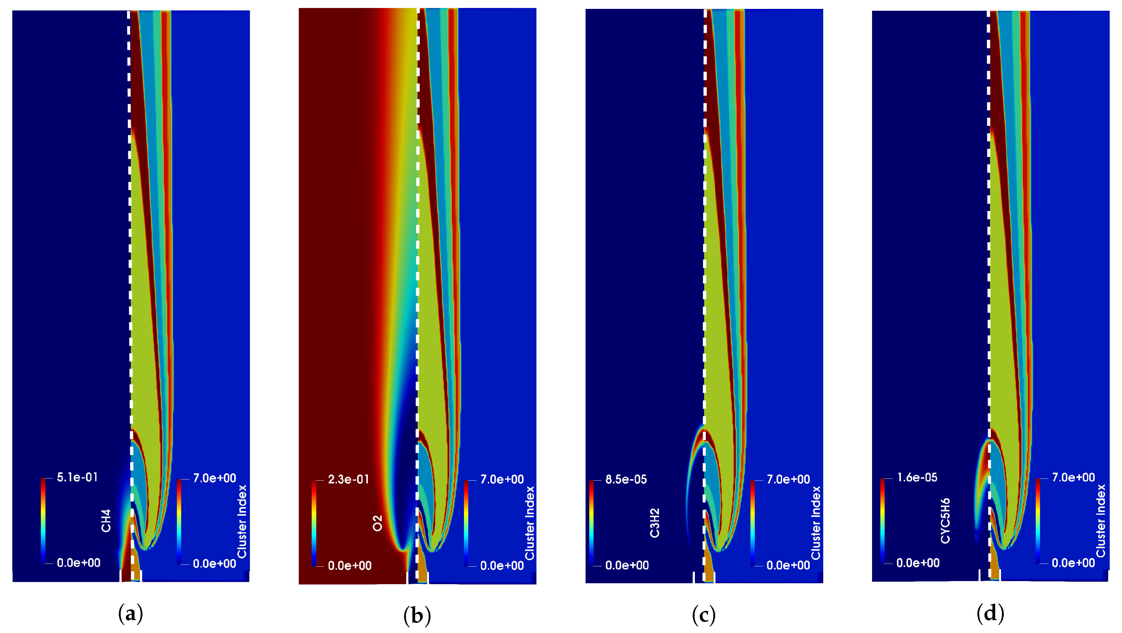
In Figure 1, an example of the cluster classification in time is shown for several timesteps of a 2D unsteady coflow methane flame adaptive simulation, while in Figure 2 the clustering (referring to the timestep t = 0.0025 s) is compared with the mass fraction profiles of some of the chemical species for the same timestep. From these two figures it is possible to see that, although the thermochemical space classification is only driven by mathematical metrics in a high-dimensional space, the physical coherence is kept.

2.2. Self Organizing Maps

Self Organizing Maps (SOMs) are a type of artificial neural networks widely used for exploratory analysis of high-dimensional data. SOMs allow to perform a non-linear mapping between a high-dimensional space and a two-dimensional (2D) map in a totally unsupervised fashion [14,15]. The mapping is able to preserve the topology of the original space, which means that the points close to each other in the original space remain closely located in the 2D map. The SOM is made up of neurons arranged in a 2D lattice, each of them storing a weight vector having the same dimensions of the input space.
Considering a training matrix X consisting of n rows (observations) and p columns (variables), there are two parameters to be set in order to perform the high-dimensional space mapping with a SOM: the first one is the total number of neurons, the second one is the geometry of the map. With regard to the first parameter, Vesanto et al. [16] estimated N = 5 n as a good number of neurons to be used in a two-level approach. The geometry of the map can instead be calculated computing the first two eigenvalues of the dataset, as from their ratio the number of neurons on the two sides of the map ( n 1 and n 2 , respectively) can be calculated [17].
If a multivariate dataset is considered for the mapping, data must be standardized before applying the algorithm: the centering factor of the j-th variable must be subtracted to each observation (centering), then the centered observation must be divided by a prescribed scaling factor to normalize variables which have different units and ranges (scaling). The centered and scaled i-th observation of the j-th variable ( x ˜ i , j ) will be then obtained as: x ˜ i , j = x i , j x ¯ j d j . Several scaling criteria are available in statistics for multivariate datasets, and their effects have already been documented for combustion applications [18]. In this work, the Auto scaling criterion was used before applying the examined partitioning algorithms: the variables were centered with their mean values and scaled with their standard deviations, as it allows to consider evenly all the variables [18].

2.3. K-Means Clustering

The K-Means clustering [19,20] is an iterative algorithm capable of efficiently partitioning n observations of a dataset into k groups (clusters), whose number is a priori defined by the user. The clusters are initially randomly allocated, but at each iteration the position of the center of each cluster, the centroid vector c ¯ k , is shifted to minimize an error function, defined as the sum of squared euclidean distances between the set of observations belonging to a k-th cluster and the centroid of the cluster c ¯ k itself. The convergence of the algorithm is achieved when the position of the centroids is not changing between two consecutive iterations, i.e., is below a fixed threshold ϵ .
While the possibility to automatically partition the data is very attractive, this method has two major drawbacks: it is not possible to find any prescribed criterion to efficiently set a priori the number of clusters k, and the random initialization of the centroids vectors can lead to local, non-optimal, minimum values of the error function, compromising the clustering results. Even if no criterion is given to set k a priori, many indices are available in literature to assist the user a posteriori for the choice of the optimal number of clusters [21,22,23,24]. With respect to the initialization issue, a possible strategy is to run the algorithm several times and choose the best clustering option, i.e., the one which is characterized by the lowest error.

2.4. Coupling SOM with K-Means

Given the relation between the number of observations in the dataset and the number of neurons in a SOM, it is clear that even for relatively small datasets (thousands of observations) the number of neurons can be extremely high. Thus, although this aspect strengthens the ability of the SOM to efficiently map the high-dimensional space, it could be undesirable for clustering purposes. In fact, the number of clusters could be overestimated if compared to the number of observations: the population in each cluster could be too low to have any statistical or physical meaning. For this reason, this technique can be coupled with a clustering algorithm to group the closest neurons, ultimately obtaining the prescribed number of clusters required for the specific application after the mapping, as described in [16,17,25].
In order to group the neurons with a clustering algorithm, a dissimilarity matrix Δ containing the distances between each neuron and the n observations of the dataset must be calculated first [25].
Δ = | | x 1 w 1 | | 2 | | x 1 w q | | 2 | | x n w 1 | | 2 | | x n w q | | 2
The K-Means algorithm can be then applied to this matrix to group the observations into k bins on the basis of their distances from the neurons, finally getting the prescribed number of clusters for the dataset.

2.5. Local Principal Component Analysis

Local Principal Component Analysis (LPCA) is a dimensionality reduction technique which was originally conceived to reduce the errors arising from the PCA intrinsic linearity [26]. The algorithm partitions the input dataset in k different disjoint regions (clusters), and in each of them PCA is performed. The input-space partitioning is achieved in a totally unsupervised fashion, by means of an iterative algorithm which uses the PCA reconstruction error minimization as objective function. The PCA reconstruction error [27,28] is defined as the difference between the original ( x i ) and the reconstructed ( x ˜ i ) observation from the PCA reduced-dimensionality space:
ϵ r = | | x ˜ i x i | |
If the original, centered and scaled, data matrix X R p is partitioned in k clusters, and in each cluster PCA is performed, it is possible to find k reduced basis of eigenvectors (LPCs) A ( j ) R q , with j [ 1 , , k ] and q < p . Thus, for each observation x X it is possible to iteratively compute k reconstruction errors, and assign it to a cluster k ¯ such that:
k ¯ ϵ r , k ¯ = min j = 1 , k ϵ r , j .
The overall algorithm can be outlined as the following:
  • Initialization: the clusters’ centroids are initialized;
  • Partitioning: each observation from the training matrix is assigned to a cluster by means of Equation (3);
  • Update: the clusters’ centroids position is updated according to the new partitioning;
  • Local PCA: Principal Component Analysis is performed in each cluster.
The steps from 2 to 4 are repeated iteratively until a convergence criterion is satisfied, i.e., the reconstruction error of the full data matrix X is below a fixed threshold or the centroids’ position variation is below a fixed threshold. With respect to PCA, this method has the advantage to be locally linear instead of globally linear, being in this way capable of having a lower error arising from the dimensionality reduction in case of data obtained from non-linear systems, such as combustion data [29,30,31].
In the context of the adaptive-chemistry simulations with SPARC, the LPCA objective function can be used for both the pre-partitioning and the on-the-fly classification steps, as described in [11]. In fact, after the training dataset clustering step, a new, unobserved, vector y R p can be projected on the k local manifolds spanned by the training matrix LPCs, A ( j ) , and thus it can be assigned to the cluster k ^ such that:
k ^ ϵ r , k ^ = min j = 1 , k ϵ r , j

2.6. Directed Relation Graph with Error Propagation

In order to convey the information included in detailed chemistry to CFD applications, the use of skeletal reduction techniques is often a necessary step, thus in the last decades significant effort has been put on this research field. The state of the art on this topic is thoroughly described in the reviews of Lu and Law [1] and Turanyi and Tomlin [32]. The common principle behind such methodologies lies in quantifying the importance of species and/or reactions composing the detailed mechanism in the defined operating conditions, such that the least important of them can be safely removed without any significant loss in the chemistry accuracy. The first works on this topic were focused on the identification and removal of unimportant reactions, either via Sensitivity Analysis [33,34] or Principal Component Analysis [35,36]. A major breakthrough was obtained with the development of reduction approaches aimed at removing unimportant species. In particular, approaches based on flux analysis proved to be particularly effective to classify the species importance according to the operating conditions, in reasonable times. The most impactful works in this field were the Directed Relation Graph (DRG) devised by Lu and Law [37], and the Directed Relation Graph with Error Propagation (DRGEP), developed by Pepiot-Desjardins and Pitsch [10]. Further evolutions refined the selection of important species via sensitivity analysis [38,39], although at a computational cost considerably higher. All of the DRG-derived approaches are based on the selection of representative reaction states in 0D/1D reactors: for each state, the interactions between species are represented via a graph-based methodology, where species represent the vertices and edges intensity depends on the reactions. Then, interaction coefficients ranking species importance are evaluated by selecting specific targets (usually fuel, oxidizer and main reaction products), and evaluating a comprehensive index (between 0 and 1) estimating the importance of each species for the formation/consumption of each target. In this work, the DRGEP approach was implemented, coupled with the Dijkstra’s shortest path algorithm [40] for an efficient calculation of the interaction coefficients. In short, such coefficients are evaluated starting from the composition of each grid point: the importance of a given B species in the formation of another A species is evaluated as:
r A B = | j = 1 N R ν A j ω j δ j | m a x ( P A , C A )
where P A and C A are the formation and consumption rates of A, respectively, δ j is a boolean variable indicating the presence of B in the j-th reaction, ν A j is the stoichiometric coefficient of A in the j-th reaction and ω j is the local j-th reaction rate. After defining fuel and oxidizer as target species, an interaction coefficient along the p-th reaction pathway is evaluated:
r A B , p = i = 1 n p 1 r S i , S i + 1
where S i is the i-th species along the p-th reaction pathway. The overall interaction coefficient quantifying the importance of B in the formation of A is evaluated considering the maximum of Equation (6) along all the pathways:
R A B = max p ( r A B , p )
and the final coefficient representing the importance of B in the single grid point is evaluated by considering all the target species:
R ˜ B = max X R X B , p

3. Case Description

The partitioning for the generation of the reduced mechanisms must be done on data obtained from previous simulations of the same system or, alternatively, if an existing multi-dimensional detailed simulation of the same system is not available, from a set of 0D or 1D simulations. The necessary condition to ensure the validity of the approach is that the training dataset must cover the thermochemical space likely to be accessed during the multidimensional CFD simulation [11].
A 2D unsteady coflow laminar diffusion flame [41] was simulated with the adaptive-chemistry approach described above using the laminarSMOKE code, a CFD solver based on OpenFOAM for laminar reacting flows [13]. This solver is based on an operator-splitting technique [12]: at each time-step, the equations for diffusion and convection for each species are firstly solved (transport sub-step), and only after the chemistry is solved (chemistry sub-step). The fuel consisted of a methane stream diluted with nitrogen (65% CH4 and 35% N2, on molar basis) and the oxidizer was air; the former was injected into the domain at 35 cm/s through a circular nozzle with internal diameter of 4 mm, while the air was injected through an annular region with internal diameter of 50 mm. Both streams were fed at ambient temperature and atmospheric pressure. The flame unsteady behavior was obtained by means of a continuous sinusoidal perturbation in the fuel parabolic velocity profile:
v r ( r , t ) = v m a x ( 1 r 2 R 2 ( 1 + A s i n ( 2 π f t ) ) ) ,
with r being the radial coordinate, R the internal radius, t the considered timestep, v m a x = 70 cm/s, f= 10 Hz and A = 0.25.
The 2D geometry was rectangular (54 mm and 120 mm in the radial and axial directions, respectively), and after a mesh sensitivity analysis it was discretized through a cartesian mesh, whose dimension was set to 25,000 cells. With regard to the chemical kinetics, the POLIMI C1C3 HT 1412 [42], accounting for 84 species and 1698 reactions, was used for the simulations.
The dataset used for the offline training (i.e., steps 1,2 and 3 described in Section 2.1) consisted of 50,000 observations randomly sampled from selected timesteps of the 2D detailed simulation of the same reacting system. Before applying the machine learning algorithms, the accessed thermochemical spaces (of the full and the sampled training datasets, respectively) were compared to assess the quality of the sampling, as done in Figure 3. In fact, as already shown in [11], a necessary condition to assure a good accuracy for the SPARC adaptive simulation is that the training dataset is covering the thermochemical space which will be accessed during the adaptive simulation.
The CFD simulations were carried out by adopting both the detailed mechanism and the adaptive-chemistry approach, to have a proper comparison both in terms of accuracy and speed-up.

4. Results

4.1. Adaptive Simulation with SKM Partitioning

The training dataset was initially mapped with a SOM, as described in Section 2.2. After such mapping, the distances between the neurons and the dataset observations were computed to build the matrix Δ to partition with the K-Means algorithm. To set the number of clusters k, the Davies-Bouldin (DB) index [21] was computed to choose the optimal number of groups ( k o p t ) for the partitioning. Because of the K-Means algorithm sensitivity to the initial conditions, due to the random centroids initialization step, five partitioning were carried out with k o p t and the one with the lowest error score was chosen. The SOM used for the mapping consisted of 38 × 30 neurons, and k o p t was found to be equal to 8. After the partitioning, a reduced kinetic mechanism was generated for each cluster combining each reduced mechanism obtained for each of its points. In order to have the possibility to evaluate from a chemical point of view the quality of the generated reduced mechanisms, the same non-uniformity coefficient λ , defined in [11], was used. This coefficient can take values in a range between 0 and 1, being equal to 0 if all the individual mechanisms of the points in a cluster are identical, i.e., the mechanisms are perfectly uniform in terms of species, and 1 in case of complete non-uniformity. In Table 1 the mean, as well as the minimum and the maximum number of species in each cluster ( n s p m e a n , n s p m i n and n s p m a x , respectively) and the corresponding mean non-uniformity coefficient ( λ m e a n ) are reported for the partitioning carried out using the number of clusters prescribed by the DB index, with a reduction tolerance ϵ D R G E P equal to 0.005 and fuel and oxidizer as target species.
Examining the statistics reported in Table 1, it is possible to observe that the chemical reduction in the number of species was about the 50%, despite the relatively low DRGEP tolerance. Moreover, it is important to highlight that with a global reduction for the same system, on equal terms of tolerance ϵ D R G E P , it was possible to reduce the number of species only up to 59, as shown in [11].
For the on-the-fly classification task with regard to the SKM partitioning adaptive simulation, an ANN classifier was trained in the pre-processing stage and then integrated in the CFD solver. The network architecture consisted of two hidden layers with 50 neurons each, using a batch size of 512 observations, and categorical crossentropy as loss function. For both the hidden layers a Rectified Linear Unit (ReLU) activation function was adopted, while for the output layer a softmax activation function was chosen, as prescribed for classification tasks. The softmax function allows to compute a score for the class membership probability, and the class with the highest probability is assigned to the considered observation. The architecture and the hyperparameters were set after an accurate offline tuning process. To avoid the network overfitting, the initial dataset was split in a training-set (75% of the total number of observations) and a test-set (with the remaining 25% of the total number of observations) in the offline training stage of the ANN. Moreover, early stopping was adopted: this technique allows to stop the training phase in advance if the classification performances of the test-set reach a plateau [43], and the implemented architecture is also capable to learn a model similar to the one which would have been learned by an optimal-sized one [43].
An adaptive CFD simulation of the 2D laminar flame described in Section 3 was carried out using the library of the aforementioned reduced mechanisms. The analysis of the adaptive-chemistry simulation performances consisted of two steps. Firstly, a quantitative error assessment was performed, examining the normalized root mean squared errors (NRMSE = 1 y ¯ · i = 1 N ( y ^ i y i ) 2 N , with y ^ i and y i being the real and the value obtained by means of the adaptive approach, respectively, and y ¯ the mean value of the measured variable throughout the field) between the detailed and the adaptive simulations for several selected species. Subsequently, a speed-up assessment was carried out, monitoring the speed-up factor ( S c h e m m e a n ) for the adaptive approach.
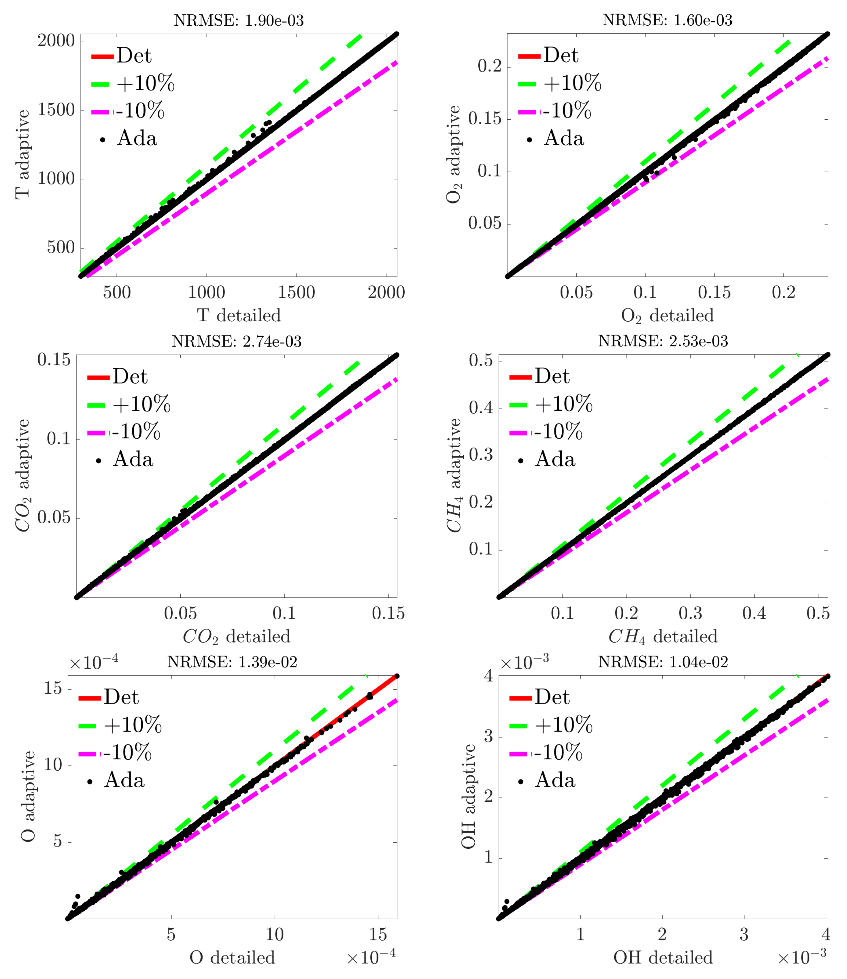
In Figure 4, the parity plots and the NRMSEs are reported for t = 0.03 s for some of the selected species, for the adaptive simulation with reduced mechanisms obtained from the SKM partitioning with Auto scaling. The adaptive simulation results to be very accurate, as the mean error on the entire domain is between ∼ 10 3 and 10 2 for both stable species and radicals, and the error rarely goes above and below the green and purple lines, therefore staying mostly bounded in the ± 10 % error region. Because of the unsteadiness of the considered simulation, the error for several selected variables (i.e. T, O2, H2O, CO, CO2, CH4, O, OH) was also averaged to monitor its behavior in time. As shown in Figure 5, the average error of the adaptive simulation does not amplify in time, staying always bounded in the range of 10 3 .
With regard to the computational speed-up, the overall speed-up factor for the adaptive simulation compared to the detailed one ( S c h e m ) was also monitored in time. In fact, since the flame physics changes in time, the number of species and reactions can also change depending on the timestep, thus resulting in a different S c h e m . In Figure 6, the average speed-up, as well as the average number of species and reactions in time, are reported. The adaptive simulation was characterized by a speed-up factor S c h e m between ∼3.9 and ∼4.3, and its behavior directly reflects the one of the number of species.

4.2. Adaptive Simulation with LPCA Partitioning

To assess the performances of the CFD adaptive simulation using the reduced mechanisms obtained by means of the LPCA clustering, the thermochemical space partitioning was again carried out on the same training dataset scaled with Auto scaling criterion. Also in this case, the partitioning and the generation of the reduced mechanisms were carried out with k = 8 and tolerance ϵ D R G E P = 0.005 , respectively, as previously done in the hybrid SKM approach. The equality in terms of number of clusters and reduction tolerance threshold is required to allow a fair comparison for the two partitioning algorithms, as the reduction (i.e., the mean number of species and their uniformity) is sensitive to the given number of classes, as shown in [11].
In Table 2, the statistics of the reduction with the DRGEP, i.e., the mean, the minimum and the maximum number of species, as well as the non-uniformity coefficient, are shown for the LPCA partitioning. As it is possible to observe from Table 2, the LPCA partitioning led to a similar reduction with respect to the number of species obtained by means of the SKM approach, although a lower minimum number of species was obtained. Moreover, the value of the mean non-uniformity coefficient decreased of ∼18% with respect to the previous reduction. These two results are already a good basis for the comparison between the two clustering methods. The difference in the minimum number of species can have a strong influence on the simulation speed-up, considering that this difference involves the cluster with more grid-points in the simulation (the region outside the flame) and, therefore, even a minimal difference in terms of species can be translated into a larger speed-up if multiplied for a large number of cells. Also examining the λ m e a n value, it is clear that the partitioning via LPCA leads to more homogeneous reduced mechanisms as its value is about the ∼18% lower than the one obtained by means of the SKM partitioning.
In addition to the λ coefficient, it is also possible to introduce an additional parameter to compare the goodness of the two partitioning methods. In fact, the purpose of any clustering algorithm is to isolate groups of similar points, making sure that they are as homogeneous as possible, i.e., maximizing the intra-cluster similarity. Although coefficients to evaluate the space partitioning can be easily found in literature, as also mentioned in Section 2, they all adopt geometrical distances as a metric to evaluate the intra-cluster similarity. For this application, instead, a physical criterion was considered to be more suitable, thus the Physical Homogeneity Coefficient (PHC) was introduced. The latter is defined as:
P H C = 1 n v a r i = 1 n v a r ( M i m i μ i ) ,
where M i and m i are the maximum and the minimum value of the i-th variable in the examined cluster, respectively, and μ i its mean value. From Equation (10), it is clear that the smaller the value of PHC, the more homogeneous the cluster (as well as more consistent from a physical point of view).
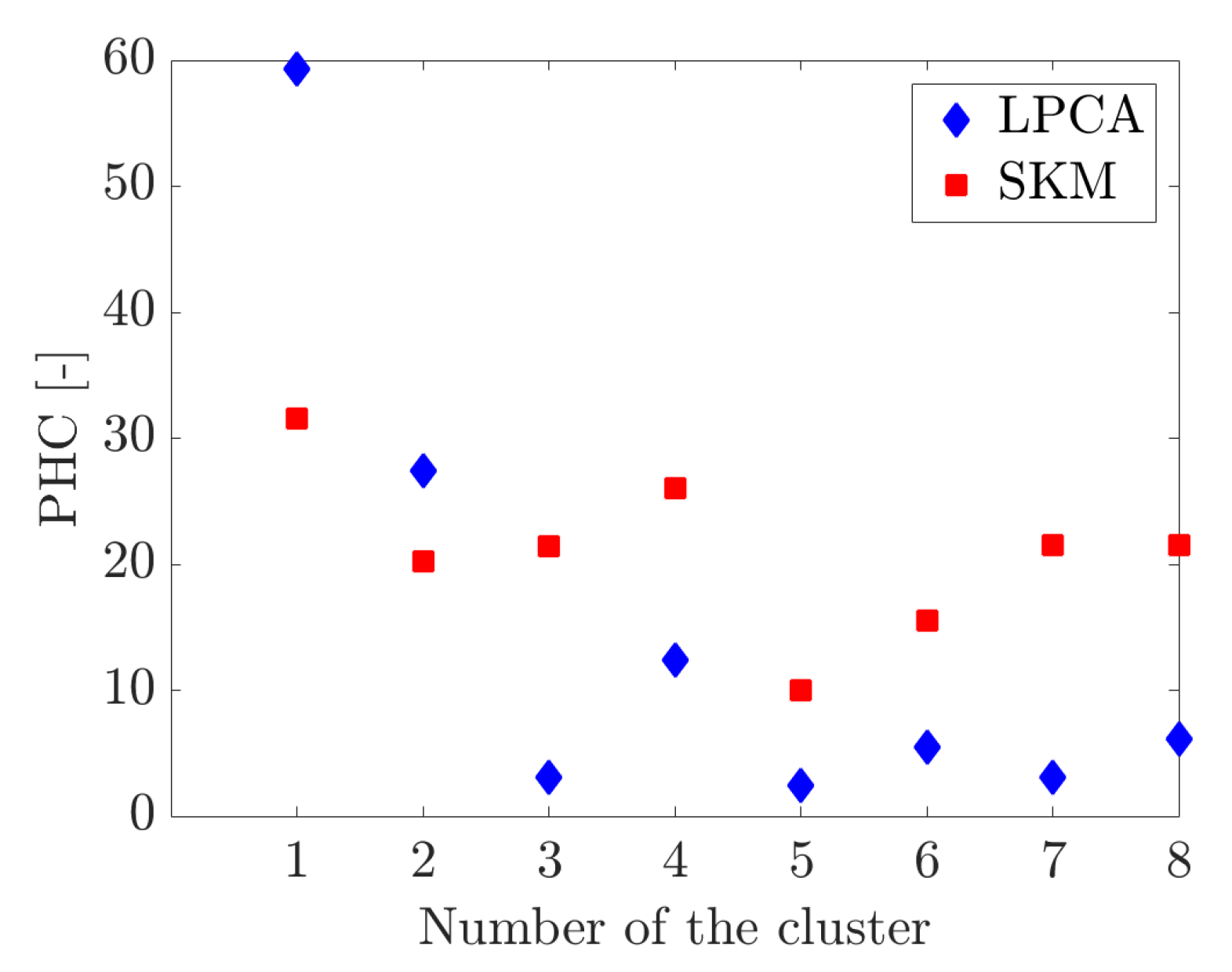
In Figure 7, the PHC in each cluster is reported for the two partitioning solutions. In all the clusters, except for clusters 1 and 2, LPCA results to be more homogeneous in terms of species mass fractions, proving again its effectiveness for clustering tasks in the context of adaptive-chemistry, with respect to the SKM algorithm.
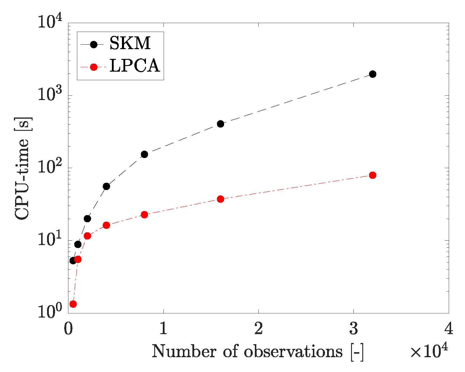
Another aspect to consider to allow a fair comparison between the two algorithms, besides the quality of the clustering solution, is their computational complexity (i.e., how the computational time required to reach convergence scales up with the training dataset dimensions). This parameter is crucial since an excessive computational complexity could compromise the application of the algorithm for large datasets. In the field of combustion, in fact, it is more and more common to develop reduced models, either global or local, from massive datasets obtained from DNS simulations of reactive jets [44,45,46,47,48], accounting for millions of observations. Moreover, also in case canonical reactors (0D or 1D) are used to generate training data for model order reduction, large datasets are anyway required to properly train the machine learning models [49,50,51]. In Figure 8, the computational time needed to reach convergence is plotted against the number of dataset observations, for a fixed number of clusters in input ( k = 8 ). Both the algorithms were tested on the same machine using MATLAB(R) (MATLAB, version 9.3.0 (R2017b). Natick, Massachusetts: The MathWorks Inc.): for SKM the built-in functions were used (for Self Organizing Maps as well as for the K-Means clustering); a in-house code was instead used for LPCA. A non-linear relation between the CPU-time and the number of observations included in the training dataset is observed for SKM as well as for LPCA, but the first algorithm appears to be much more sensitive to the data size with respect to the second one as the CPU-time difference, in case a matrix accounting for 32,000 observations, is greater than two orders of magnitude.
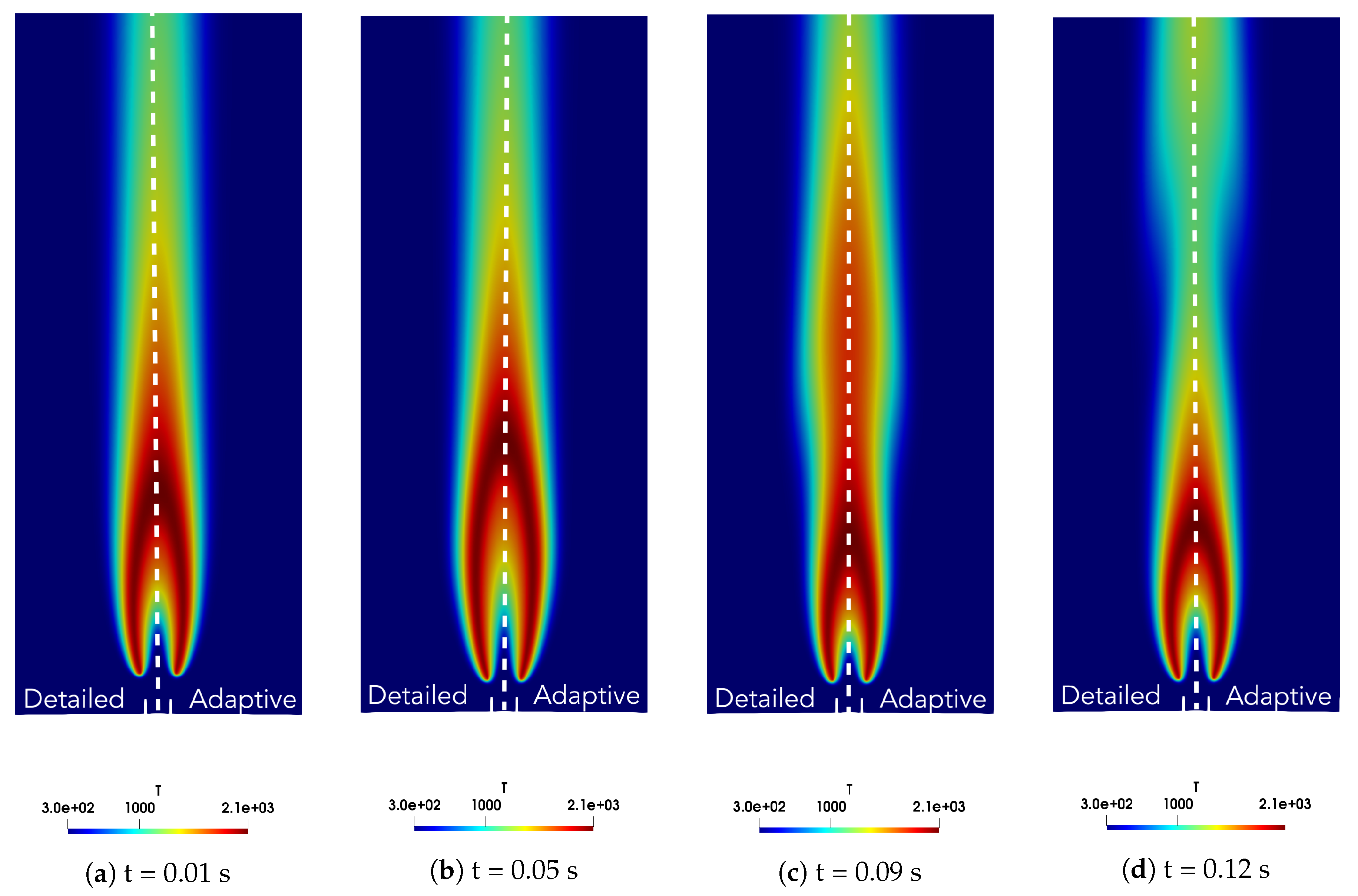
With regard to the adaptive CFD simulation with the reduced mechanisms obtained by means of the LPCA partitioning, in Figure 9 a comparison of the accuracy and the speed-up with respect to SKM is shown. A lower accuracy of the LPCA adaptive simulation is observed for all the examined timesteps with respect to the SKM simulation but, on the other hand, the LPCA adaptive simulation speed-up factor is constantly higher (∼5) than the SKM adaptive simulation (∼4).
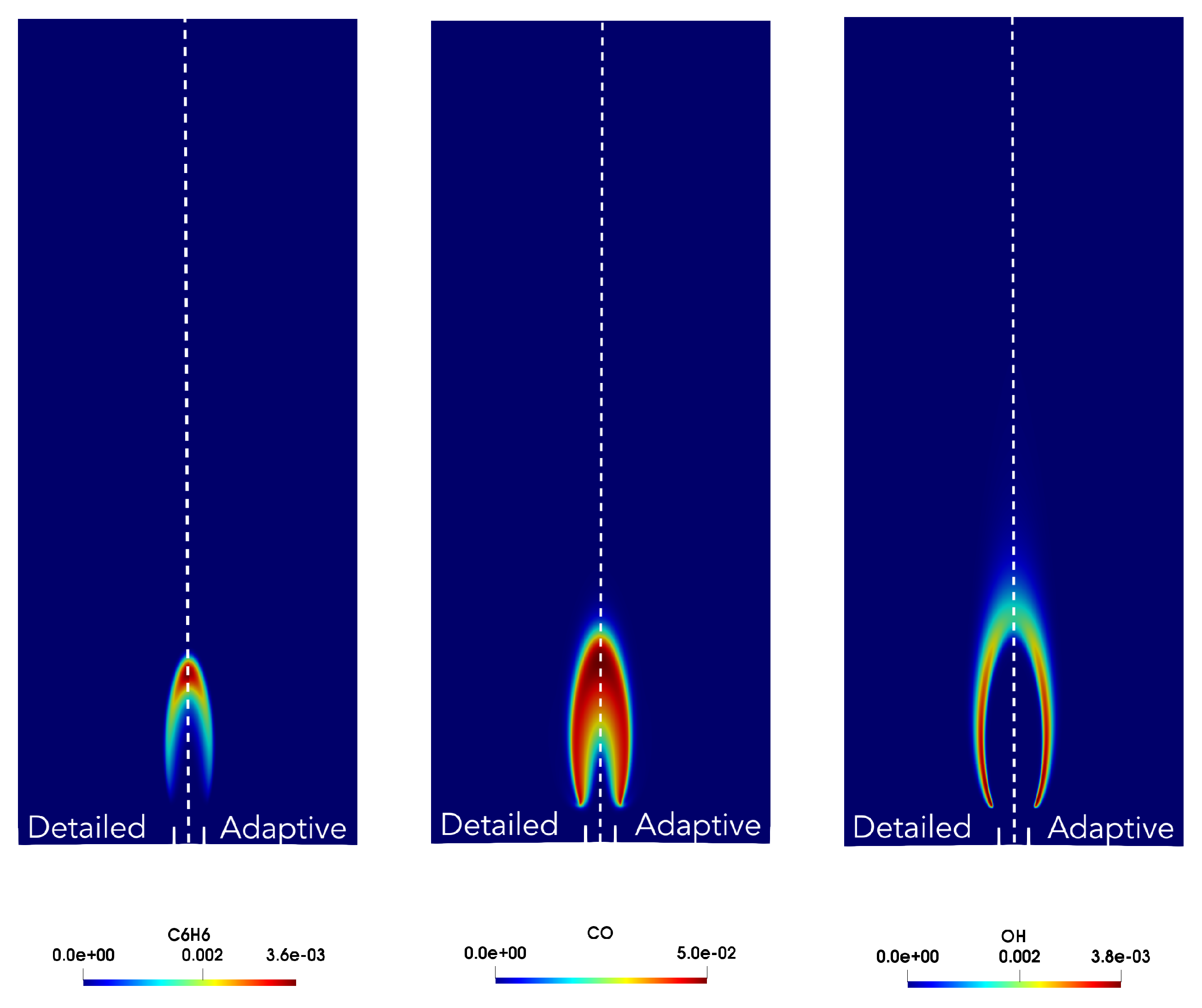
Taking into account these additional two parameters to compare the adaptive simulations, once again LPCA gave better results than SKM. In fact, the discrepancy in the accuracy between the two simulations is negligible and the errors are overall small (as also shown by the comparison of the contours between the detailed and the LPCA adaptive simulations, reported in Figure 10 and Figure 11, as the differences are hardly noticeable). On the other hand, the speed-up factor discrepancy ( 20 % ) appears to be more relevant, especially in perspective of an application to turbulent flames, where a very large number of grid points or chemical species are used, and the speed-up difference would be considerably higher.

5. Conclusions

The thermochemical space pre-partitioning covers an important role in the SPARC adaptive-chemistry approach, as it can strongly affect the adaptive CFD simulation results in terms of accuracy and computational speed-up. A good clustering can, in fact, lead to homogeneous reduced mechanisms, with a strong reduction in the mean number of species, and satisfactory performances both in terms of accuracy and speed-up. A non-optimal clustering can, instead, compromise the accuracy or the speed-up.
In this work, two clustering techniques were implemented to partition the thermochemical space and generate the reduced mechanisms to adaptively simulate a 2D unsteady laminar coflow methane flame: a hybrid SOM K-Means (SKM) approach and Local Principal Component Analysis (LPCA). Their performances were firstly assessed evaluating the reduced mechanisms’ chemical coherence (i.e., the non-uniformity coefficient λ ) and intra-cluster homogeneity (i.e., the Physical Homogeneity Coefficient), as well as the relation between the CPU-time required to reach the convergence criteria and the training matrix size. After that, their impact on the performances of the multidimensional adaptive simulation was examined, in terms of accuracy and observed speed-up with respect to the detailed simulation. Both the algorithms led to excellent results in terms of reduced mechanisms: the reduction in terms of mean number of species was ∼50%, but LPCA led to more uniform reduced mechanisms, implying a better space-state partitioning. This result was confirmed in second instance by means of the Physical Homogeneity Coefficient (PHC): the 75% of the clusters found LPCA resulted to be more coherent, from a physical point of view, with respect to the SKM ones. Moreover, the local algorithm proved to be less sensitive than SKM to the training dataset dimensions in terms of CPU-time required to reach convergence. The SKM adaptive simulation was slightly more accurate, but LPCA had superior performances in terms of speed-up (∼5).

Author Contributions

Conceptualization, G.D., A.C. and A.P.; software, G.D., G.A., A.S., A.P. and A.C.; investigation, G.D.; writing–original draft preparation, G.D.A. and A.S.; writing–review and editing, A.C., A.S., M.B., G.A. and A.P.; supervision, A.C. and A.P.; funding acquisition, A.P. All authors have read and agreed to the published version of the manuscript.

Funding

The first author has received funding from the Fonds National de la Recherche Scientifique (FRS-FNRS) through a FRIA fellowship. This research has received funding from the European Research Council (ERC) under the European Union’s Horizon 2020 research and innovation programme under grant agreement No 714605.

Acknowledgments

We acknowledge the CINECA award under the ISCRA initiative, for the availability of high performance computing resources and support (ISCRA-B: HP10BGXWCZ).

Conflicts of Interest

The authors declare no conflict of interest.

References

  1. Lu, T.; Law, C.K. Toward accommodating realistic fuel chemistry in large-scale computations. Prog. Energy Combust. Sci. 2009, 35, 192–215. [Google Scholar] [CrossRef]
  2. Fang, X.; Huang, Z.; Qiao, X.; Ju, D.; Bai, X. Skeletal mechanism development for a 3-component jet fuel surrogate using semi-global sub-mechanism construction and mechanism reduction. Fuel 2018, 229, 53–59. [Google Scholar] [CrossRef]
  3. Chen, Y.; Mehl, M.; Xie, Y.; Chen, J.Y. Improved skeletal reduction on multiple gasoline-ethanol surrogates using a Jacobian-aided DRGEP approach under gasoline compression ignition (GCI) engine conditions. Fuel 2017, 210, 617–624. [Google Scholar] [CrossRef]
  4. Ranade, R.; Alqahtani, S.; Farooq, A.; Echekki, T. An extended hybrid chemistry framework for complex hydrocarbon fuels. Fuel 2019, 251, 276–284. [Google Scholar] [CrossRef]
  5. Liang, L.; Stevens, J.G.; Farrell, J.T. A dynamic adaptive chemistry scheme for reactive flow computations. Proc. Combust. Inst. 2009, 32, 527–534. [Google Scholar] [CrossRef]
  6. Contino, F.; Jeanmart, H.; Lucchini, T.; D’Errico, G. Coupling of in situ adaptive tabulation and dynamic adaptive chemistry: An effective method for solving combustion in engine simulations. Proc. Combust. Inst. 2011, 33, 3057–3064. [Google Scholar] [CrossRef]
  7. Zhou, L.; Wei, H. Chemistry acceleration with tabulated dynamic adaptive chemistry in a realistic engine with a primary reference fuel. Fuel 2016, 171, 186–194. [Google Scholar] [CrossRef]
  8. Komninos, N. An algorithm for the adaptive run-time reduction of chemical mechanisms during HCCI simulation. Fuel 2015, 140, 328–343. [Google Scholar] [CrossRef]
  9. Newale, A.S.; Liang, Y.; Pope, S.B.; Pepiot, P. A combined PPAC-RCCE-ISAT methodology for efficient implementation of combustion chemistry. Combust. Theory Model. 2019, 23, 1–33. [Google Scholar] [CrossRef]
  10. Pepiot-Desjardins, P.; Pitsch, H. An efficient error-propagation-based reduction method for large chemical kinetic mechanisms. Combust. Flame 2008, 154, 67–81. [Google Scholar] [CrossRef]
  11. D’Alessio, G.; Parente, A.; Stagni, A.; Cuoci, A. Adaptive chemistry via pre-partitioning of composition space and mechanism reduction. Combust. Flame 2020, 211, 68–82. [Google Scholar] [CrossRef]
  12. Ren, Z.; Pope, S.B. Second-order splitting schemes for a class of reactive systems. J. Comput. Phys. 2008, 227, 8165–8176. [Google Scholar] [CrossRef]
  13. Cuoci, A.; Frassoldati, A.; Faravelli, T.; Ranzi, E. Numerical modeling of laminar flames with detailed kinetics based on the operator-splitting method. Energy Fuels 2013, 27, 7730–7753. [Google Scholar] [CrossRef]
  14. Kohonen, T. The self-organizing map. Proc. IEEE 1990, 78, 1464–1480. [Google Scholar] [CrossRef]
  15. Kohonen, T.; Oja, E.; Simula, O.; Visa, A.; Kangas, J. Engineering applications of the self-organizing map. Proc. IEEE 1996, 84, 1358–1384. [Google Scholar] [CrossRef]
  16. Vesanto, J.; Alhoniemi, E. Clustering of the self-organizing map. IEEE Trans. Neural Netw. 2000, 11, 586–600. [Google Scholar] [CrossRef]
  17. Garcia, H.L.; Gonzalez, I.M. Self-organizing map and clustering for wastewater treatment monitoring. Eng. Appl. Artif. Intell. 2004, 17, 215–225. [Google Scholar] [CrossRef]
  18. Parente, A.; Sutherland, J.C. Principal component analysis of turbulent combustion data: Data pre-processing and manifold sensitivity. Combust. Flame 2013, 160, 340–350. [Google Scholar] [CrossRef] [Green Version]
  19. Lloyd, S. Least squares quantization in PCM. IEEE Trans. Inf. Theory 1982, 28, 129–137. [Google Scholar] [CrossRef]
  20. MacQueen, J. Some methods for classification and analysis of multivariate observations. In Proceedings of the Fifth Berkeley Symposium on Mathematical Statistics and Probability; University of California: Oakland, CA, USA, 1967; Volume 1, pp. 281–297. [Google Scholar]
  21. Davies, D.L.; Bouldin, D.W. A cluster separation measure. IEEE Trans. Pattern Anal. Mach. Intell. 1979, PAMI-1, 224–227. [Google Scholar] [CrossRef]
  22. Caliński, T.; Harabasz, J. A dendrite method for cluster analysis. Commun. Stat. Theory Methods 1974, 3, 1–27. [Google Scholar] [CrossRef]
  23. Rousseeuw, P.J. Silhouettes: A graphical aid to the interpretation and validation of cluster analysis. J. Comput. Appl. Math. 1987, 20, 53–65. [Google Scholar] [CrossRef] [Green Version]
  24. Tibshirani, R.; Walther, G.; Hastie, T. Estimating the number of clusters in a data set via the gap statistic. J. R. Stat. Soc. Ser. B Stat. Methodol. 2001, 63, 411–423. [Google Scholar] [CrossRef]
  25. Brentan, B.; Meirelles, G.; Luvizotto, E., Jr.; Izquierdo, J. Hybrid SOM+ k-Means clustering to improve planning, operation and management in water distribution systems. Environ. Model. Softw. 2018, 106, 77–88. [Google Scholar] [CrossRef]
  26. Kambhatla, N.; Leen, T.K. Dimension reduction by local principal component analysis. Neural Comput. 1997, 9, 1493–1516. [Google Scholar] [CrossRef]
  27. Jolliffe, I. Principal Component Analysis; Springer: Berlin, Germany, 2011. [Google Scholar]
  28. Bishop, C.M. Pattern Recognition and Machine Learning; Springer: Berlin, Germany, 2006. [Google Scholar]
  29. Parente, A.; Sutherland, J.; Dally, B.; Tognotti, L.; Smith, P. Investigation of the MILD combustion regime via principal component analysis. Proc. Combust. Inst. 2011, 33, 3333–3341. [Google Scholar] [CrossRef]
  30. Parente, A.; Sutherland, J.C.; Tognotti, L.; Smith, P.J. Identification of low-dimensional manifolds in turbulent flames. Proc. Combust. Inst. 2009, 32, 1579–1586. [Google Scholar] [CrossRef] [Green Version]
  31. Aversano, G.; Bellemans, A.; Li, Z.; Coussement, A.; Gicquel, O.; Parente, A. Application of reduced-order models based on PCA & Kriging for the development of digital twins of reacting flow applications. Comput. Chem. Eng. 2019, 121, 422–441. [Google Scholar]
  32. Turányi, T.; Tomlin, A.S. Analysis of Kinetic Reaction Mechanisms; Springer: Berlin, Germany, 2014. [Google Scholar]
  33. Rabitz, H.; Kramer, M.; Dacol, D. Sensitivity analysis in chemical kinetics. Annu. Rev. Phys. Chem. 1983, 34, 419–461. [Google Scholar] [CrossRef]
  34. Tomlin, A.S.; Pilling, M.J.; Merkin, J.H.; Brindley, J.; Burgess, N.; Gough, A. Reduced mechanisms for propane pyrolysis. Ind. Eng. Chem. Res. 1995, 34, 3749–3760. [Google Scholar] [CrossRef]
  35. Brown, N.J.; Li, G.; Koszykowski, M.L. Mechanism reduction via principal component analysis. Int. J. Chem. Kinet. 1997, 29, 393–414. [Google Scholar] [CrossRef]
  36. Vajda, S.; Turányi, T. Principal component analysis for reducing the Edelson-Field-Noyes model of the Belousov-Zhabotinskii reaction. J. Phys. Chem. 1986, 90, 1664–1670. [Google Scholar] [CrossRef]
  37. Lu, T.; Law, C.K. A directed relation graph method for mechanism reduction. Proc. Combust. Inst. 2005, 30, 1333–1341. [Google Scholar] [CrossRef]
  38. Zheng, X.; Lu, T.; Law, C.K. Experimental counterflow ignition temperatures and reaction mechanisms of 1, 3-butadiene. Proc. Combust. Inst. 2007, 31, 367–375. [Google Scholar] [CrossRef]
  39. Niemeyer, K.E.; Sung, C.J.; Raju, M.P. Skeletal mechanism generation for surrogate fuels using directed relation graph with error propagation and sensitivity analysis. Combust. Flame 2010, 157, 1760–1770. [Google Scholar] [CrossRef] [Green Version]
  40. Dijkstra, E.W. A note on two problems in connexion with graphs. Numer. Math. 1959, 1, 269–271. [Google Scholar] [CrossRef] [Green Version]
  41. Mohammed, R.; Tanoff, M.; Smooke, M.; Schaffer, A.; Long, M. Computational and experimental study of a forced, time-varying, axisymmetric, laminar diffusion flame. Symp. Int. Combust. 1998, 27, 693–702. [Google Scholar] [CrossRef]
  42. Ranzi, E.; Frassoldati, A.; Stagni, A.; Pelucchi, M.; Cuoci, A.; Faravelli, T. Reduced kinetic schemes of complex reaction systems: Fossil and biomass?derived transportation fuels. Int. J. Chem. Kinet. 2014, 46, 512–542. [Google Scholar] [CrossRef]
  43. Caruana, R.; Lawrence, S.; Giles, C.L. Overfitting in neural nets: Backpropagation, conjugate gradient, and early stopping. In Advances in Neural Information Processing Systems; MIT Press: Cambridge, MA, USA, 2001; pp. 402–408. [Google Scholar]
  44. Wick, A.; Attili, A.; Bisetti, F.; Pitsch, H. DNS-driven analysis of the Flamelet/Progress Variable model assumptions on soot inception, growth, and oxidation in turbulent flames. Combust. Flame 2020, 214, 437–449. [Google Scholar] [CrossRef]
  45. Swaminathan, N. Physical Insights on MILD combustion from DNS. Front. Mech. Eng. 2019, 5, 59. [Google Scholar] [CrossRef]
  46. Luo, Z.; Yoo, C.S.; Richardson, E.S.; Chen, J.H.; Law, C.K.; Lu, T. Chemical explosive mode analysis for a turbulent lifted ethylene jet flame in highly-heated coflow. Combust. Flame 2012, 159, 265–274. [Google Scholar] [CrossRef]
  47. Trisjono, P.; Pitsch, H. Systematic analysis strategies for the development of combustion models from DNS: A review. Flow Turbul. Combust. 2015, 95, 231–259. [Google Scholar] [CrossRef]
  48. D’Alessio, G.; Attili, A.; Cuoci, A.; Pitsch, H.; Parente, A. Analysis of turbulent reacting jets via Principal Component Analysis. In Data Analysis for Direct Numerical Simulations of Turbulent Combustion; Springer International Publishing: Cham, Switzerland, 2020. [Google Scholar]
  49. Roh, Y.; Heo, G.; Whang, S.E. A survey on data collection for machine learning: A big data-ai integration perspective. IEEE Trans. Knowl. Data Eng. 2019. [Google Scholar] [CrossRef] [Green Version]
  50. Najafabadi, M.M.; Villanustre, F.; Khoshgoftaar, T.M.; Seliya, N.; Wald, R.; Muharemagic, E. Deep learning applications and challenges in big data analytics. J. Big Data 2015, 2, 1. [Google Scholar] [CrossRef] [Green Version]
  51. Bach, S.H.; He, B.; Ratner, A.; Ré, C. Learning the structure of generative models without labeled data. In Proceedings of the 34th International Conference on Machine Learning, Sydney, Australia, 7–9 August 2017; Volume 70, pp. 273–282. [Google Scholar]
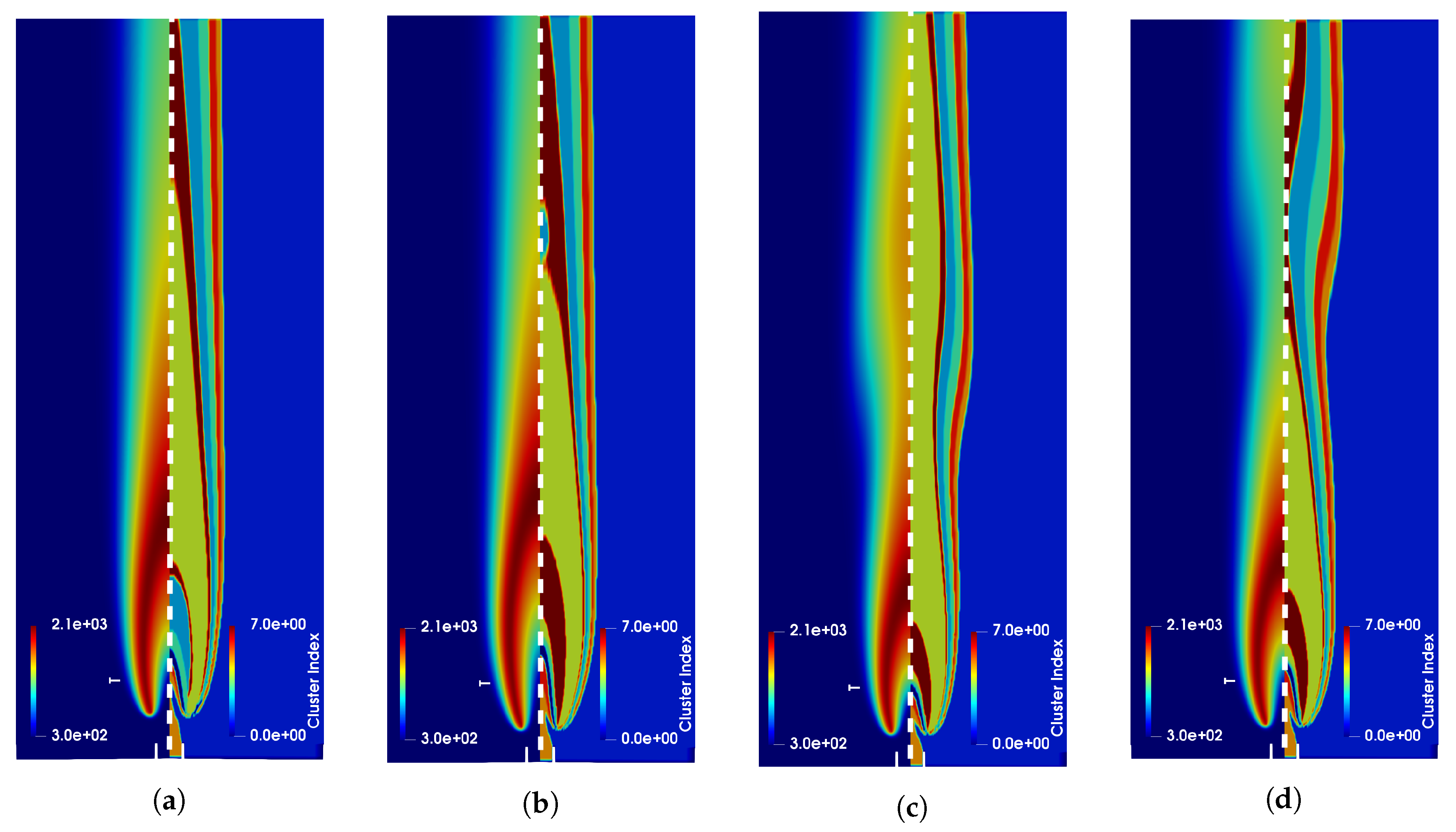
Figure 1. Maps of temperature (left part of each contour, in Kelvin) and example of the corresponding thermochemical space partitioning (right part of each contour) for timesteps of an unsteady 2D laminar coflow flame adaptive simulation: (a). t = 0.0025 s; (b). t = 0.04 s; (c). t = 0.09 s; (d). t = 0.12 s.
Energies 13 02567 g001
Figure 2. Comparison of the thermochemical space partitioning for a timestep ( t = 0.0025 s) of an unsteady 2D laminar coflow flame adaptive simulation (right part of each contour) with the maps (left part of each contour) of: (a). CH4 mass fraction; (b). O2 mass fraction; (c). C3H2 mass fraction; (d). CYC5H6 mass fraction.
Energies 13 02567 g002
Figure 3. Comparison of the accessed thermochemical space by the full (black dots) and the sampled (red cross) training dataset for: (a). CH3 mass fraction; (b). CH4 mass fraction; (c). CO mass fraction; (d). O mass fraction; (e). O2 mass fraction; (f). OH mass fraction.
Energies 13 02567 g003
Figure 4. Parity plots of temperature and selected species at t = 0.03 s for the adaptive-chemistry unsteady simulation of a 2D laminar flame with reduced mechanisms generated from the SKM clustering approach, ( ϵ D R G E P = 0.005), auto scaling criterion.
Energies 13 02567 g004
Figure 5. Averaged normalized root mean square error over time of the unsteady adaptive simulation obtained with a sinusoidal perturbation in the velocity profile ( f = 10 Hz, A = 0.25 ) with reduced mechanisms ( ϵ D R G E P = 0.005) obtained from the SKM partitioning, auto scaling criterion.
Energies 13 02567 g005
Figure 6. Statistics for several timesteps of the unsteady adaptive simulation obtained with a sinusoidal perturbation in the velocity profile ( f = 10 Hz, A = 0.25 ) with reduced mechanisms ( ϵ D R G E P = 0.005) obtained from the SKM partitioning, auto scaling criterion: (a). Mean CPU-time for the chemistry step and corresponding speed-up with respect to the detailed simulation over time; (b). Mean number of species and reactions over time.
Energies 13 02567 g006
Figure 7. Comparison of the Physical Homogeneity Coefficient (PHC) to evaluate the intra-cluster homogeneity between the SKM clustering and the LPCA clustering, on equal terms of clusters in input ( k = 8 ).
Energies 13 02567 g007
Figure 8. CPU-time (in seconds) required by the SKM algorithm (black dashed lines) and LPCA clustering algorithm (red dashed-dotted line) to reach convergence, varying the size of the training dataset with a constant number of clusters in input ( k = 8 ).
Energies 13 02567 g008
Figure 9. Comparison between the unsteady adaptive simulations obtained with a sinusoidal perturbation in the fuel velocity profile ( f = 10 Hz and A = 0.25 ) using the reduced mechanism ( ϵ D R G E P = 0.005) generated from the SKM partitioning and the LPCA partitioning: (a). Averaged normalized root mean square error over time; (b). Speed-up factor compared to detailed simulation over time.
Energies 13 02567 g009
Figure 10. Comparison of temperature maps (in Kelvin) for detailed (left part of each contour) and adaptive (right part of each contour) unsteady simulations obtained with a sinusoidal perturbation in the fuel velocity profile ( f = 10 Hz and A = 0.25 ), with reduced mechanisms obtained via LPCA pre-partitioning and ϵ D R G E P = 0.005, for several timesteps: (a). t = 0.01 s; (b). t = 0.05 s; (c). t = 0.09 s; (d). t = 0.12 s.
Energies 13 02567 g010
Figure 11. Comparison of species maps (from left to right: C6H6, CO, OH) for detailed (left part of each contour) and adaptive (right part of each contour) unsteady simulations obtained with a sinusoidal perturbation in the fuel velocity profile ( f = 10 Hz and A = 0.25 ), with reduced mechanisms obtained via LPCA pre-partitioning and ϵ D R G E P = 0.005, t = 0.12 s.
Energies 13 02567 g011
Table 1. Optimal number of clusters obtained by means of the Davies-Bouldin index ( k o p t ), mean number of species per cluster ( n s p m e a n ), minimum number of species per cluster ( n s p m i n ), maximum number of species per cluster ( n s p m e a n ) and mean non-uniformity coefficient per cluster ( λ m e a n ), using a reduction tolerance ϵ D R G E P = 0.005 for the SKM partitioning.
k opt n sp mean n sp min n sp max λ mean
84437480.093
Table 2. Number of clusters (k), mean number of species per cluster ( n s p m e a n ), minimum number of species per cluster ( n s p m i n ), maximum number of species per cluster ( n s p m a x ) and mean non-uniformity coefficient per cluster ( λ m e a n ), using a reduction tolerance ϵ D R G E P = 0.005 for the LPCA partitioning.
k n sp mean n sp min n sp max λ mean
84234490.076