A Modern Data-Mining Approach Based on Genetically Optimized Fuzzy Systems for Interpretable and Accurate Smart-Grid Stability Prediction

Abstract

The main objective and contribution of this paper was/is the application of our knowledge-based data-mining approach (a fuzzy rule-based classification system) characterized by a genetically optimized interpretability-accuracy trade-off (by means of multi-objective evolutionary optimization algorithms) for transparent and accurate prediction of decentral smart grid control (DSGC) stability. In particular, we aim at uncovering the hierarchy of influence of particular input attributes upon the DSGC stability. Moreover, we also analyze the effect of possible "overlapping" of some input attributes over the other ones from the DSGC-stability perspective. The recently published and available at the UCI Database Repository Electrical Grid Stability Simulated Data Set and its input-aggregate-based concise version were used in our experiments. A comparison with 39 alternative approaches was also performed, demonstrating the advantages of our approach in terms of: (i) interpretable and accurate fuzzy rule-based DSGC-stability prediction and (ii) uncovering the hierarchy of DSGC-system’s attribute significance.

1. Introduction

The stability of electrical grids depends on the balance between electricity generation and electricity demand. In conventional power systems, such a balance is achieved through demand-driven electricity production. Nowadays, however, due to a gradual shift from fossil-based power generation to renewable energy sources, the grid topologies are becoming more decentralized and the flow of power is becoming more bidirectional [1]. That means that consumers may function as both producers and consumers at the same time; they are often referred to as prosumers [2]. The volatile and fluctuating nature of renewable energy sources poses a significant challenge as far as design strategies and control of electric power grids are concerned. In order to balance the supply and demand in such fluctuating power grids, various smart grid approaches have been proposed. A key idea they implement is to regulate the consumers’ demand [3], usually referred to as the demand response strategy [4,5].

The changes in the consumption of electricity (in comparison with normal patterns of consumption) by customers in reaction to the changes in the price of electricity are referred to as demand response. There are two general approaches to defining the electricity price and to communicating it to consumers. A conventional approach—using costly information and communication technology infrastructure [6] is based on extensive communication between producers and consumers [7,8], raising questions, however, of cybersecurity and privacy protection [9,10]. In contrast, an alternative and novel approach referred to as decentral smart grid control (henceforward DSGC) [11] avoids massive communication between prosumers by binding the electricity price to the grid frequency which can be easily measured by means of cheap equipment by particular prosumers. During power excess, the frequency increases, whereas in times of underproduction, it decreases [12]. In that way, DSGC introduces real-time pricing allowing prosumers to easily control their momentary demand on the basis of the grid frequency. For DSGC systems to be successfully applied, they must be able to maintain grid stability for rapid changes in electricity prices and for different levels of reaction times and price sensitivity of particular grid participants [13,14].

Data mining approaches are well suited for decision support in management, control, and stability analysis of power systems including also decentralized smart grids. That is due to the availability of big amounts of simulated data on various aspects of the power systems operation; see, e.g., [15,16,17,18]. Many data mining methods have been used in the considered research field—see the next section for a brief review. However, their significant shortcoming is usually their non-transparent, black-box, and accuracy-only-oriented nature. It means that they do not provide any deeper (or any) explanations and justifications of the decisions made. As well, they do not provide any insight into mechanisms governing a given system. A similar remark has been formulated in the most recently published work [19]: "Various machine-learning and data-mining algorithms have been applied to the decentralized management and control of microgrids... Transparency is typically not the priority for most machine learning algorithms" (a quote from [19]). The present work is our attempt to address the smart-grid-stability prediction problem in an effective way by providing a solution coming from the knowledge-based data-mining field and characterized by both high interpretability and transparency and high accuracy.

The main goal and contribution of this work is the application of our knowledge-based data-mining technique, i.e., fuzzy rule-based classifiers (FRBCs) with a genetically optimized interpretability-accuracy trade-off (see, e.g., [20,21,22,23] for details) to transparent and accurate prediction of DSGC stability. In particular, we aim at uncovering the hierarchy of influence of particular input attributes upon the DSGC stability. Moreover, we will also analyze the effect of possible “overlapping” of some input attributes over the other ones from the DSGC-stability perspective. In our approach to designing FRBCs from data, measures of FRBCs’ interpretability and accuracy are treated as separate performance indices and optimization objectives. Due to their complementary/contradictory nature, we employ multi-objective evolutionary optimization algorithms (MOEOAs) in the process of the FRBCs’ structure and parameter optimization which is also equivalent to the FRBC’s interpretability-accuracy trade-off optimization (related work is reviewed in [24] and—for the case of single-objective optimization of the system—in [25,26]).

The remaining parts of the paper are organized as follows: We start with a review of related work regarding applications of data mining techniques to various aspects of electricity grid and microgrid operations. Next, the recently published Electrical Grid Stability Simulated Data Set available at the UCI Database Repository (https://archive.ics.uci.edu/ml) and its input-aggregate-based concise version proposed in [14] are characterized. Both data sets are used in our experiments. Then, main building blocks of our FRBCs are presented. Next, the FRBCs’ learning and optimization process is outlined. Two MOEOAs are independently used and compared; namely, the well-known strength Pareto evolutionary algorithm 2 (SPEA2) [27] and our generalization of SPEA2, referred to as SPEA3 [28,29,30]. In turn, the previously outlined main goal of the paper, including the application of our approach to the DSGC-stability prediction using two aforementioned simulated data sets and a comparative analysis with as many as 39 alternative approaches, is presented and discussed.

2. Related Work

Various data-mining and machine-learning models and algorithms have been applied to security, stability prediction/monitoring, management, and control of electricity grids and microgrids. An approach using an artificial neural network (ANN for short) for generating security boundaries and their visualization to transmission system operators within a power system in California is presented in [15]. The resulting security boundaries are visualized in the form of the so-called nomograms (the total number of simulations performed is equal to 1792). Extreme learning machines (ELMs for short)—a special class of ANNs—are used in [31] to improve the online learning speed and parameter tuning of the real-time transient-stability assessment model for earlier detection of the risk of blackouts. ANNs are also used to construct new monitoring methods for smart power grids. Such a method and a virtual test evaluating its performance are presented in [32]. A multilayer ANN with four hidden layers trained using a deep reinforcement learning algorithm is applied to a smart grid optimization task in [33]. In turn, a contextual anomaly detection ANN-based approach for cyber-physical security in smart grids is presented in [34]. The simulation experiments show that the contextual anomaly detection performs over 55% better than the point anomaly detection.

Support vector machines (SVMs for short) and ANNs supported by some feature selection methods are applied in [17] to the analysis of the transient stability of a large-scale Brazilian power system (the data are generated in 1242 simulation runs). SVMs and random forests (RFs for short) are used in [35] to detect smart grid devices compromised by cyber attacks. The proposed framework in different evaluation scenarios yields high accuracy (91% on average) which confirms its effectiveness at overcoming the compromised smart grid devices problem. Core vector machines (CVMs for short)—faster and big-data-oriented extensions of SVMs—are used in [36] for an online transient stability assessment of a power system by mapping that problem as a two-class classification task. An online approach makes it attractive to be used in real time applications. Genetic-algorithm-based SVMs (GA-SVMs for short) are used (and compared with conventional SVMs and ANNs) in [37] for an online voltage-stability monitoring and prediction. Their effectiveness is demonstrated by applying them to the New England 39-bus system and to the real Indian Northern Region Power Grid system.

Decision trees (DTs for short) are used (and compared with ANNs and SVMs) in [18] for prediction of the transient instability of a large-scale Iranian national grid following the test on a small 9-bus system. DTs are also used in [14] to classify the DSGC stability conditions based on the response of heterogeneous consumers to provide some insight into the relationship between the input space parameters and the grid stability.

As far as other selected data-mining techniques are concerned, the so-called active learning solution is applied in [38] to the voltage-stability prediction problem. The active learning approach interacts with the online prediction and offline training process to enhance the well-known data-mining methods (DTs, ANNs, SVMs, RFs, and radial basis function networks). In turn, modeling a non-linear security boundary by (i) using features formed as monomials of the original input up to a certain level and (ii) using kernel ridge regression to solve the problem of a large number of features is proposed in [16]. The potential of the proposed method is demonstrated by simulating the aforementioned New England 39-bus system and a larger power system with 470 buses. Next, the study [39] presents a cooperative multi-agent approach for solving the complex problems of energy management in a stand-alone solar microgrid using fuzzy logic systems and a reinforcement learning method referred to as fuzzy Q-learning. Moreover, the study [19] applies an optimized data-matching algorithm referred to as transparent open box learning network to the DSGC stability prediction. This study demonstrates the importance of compound feature selection in the considered stability prediction problem. The overwhelming majority of the above-listed studies presents the accuracy-oriented approaches. The transparency is not their priority and they usually do not provide an insight into the considered systems.

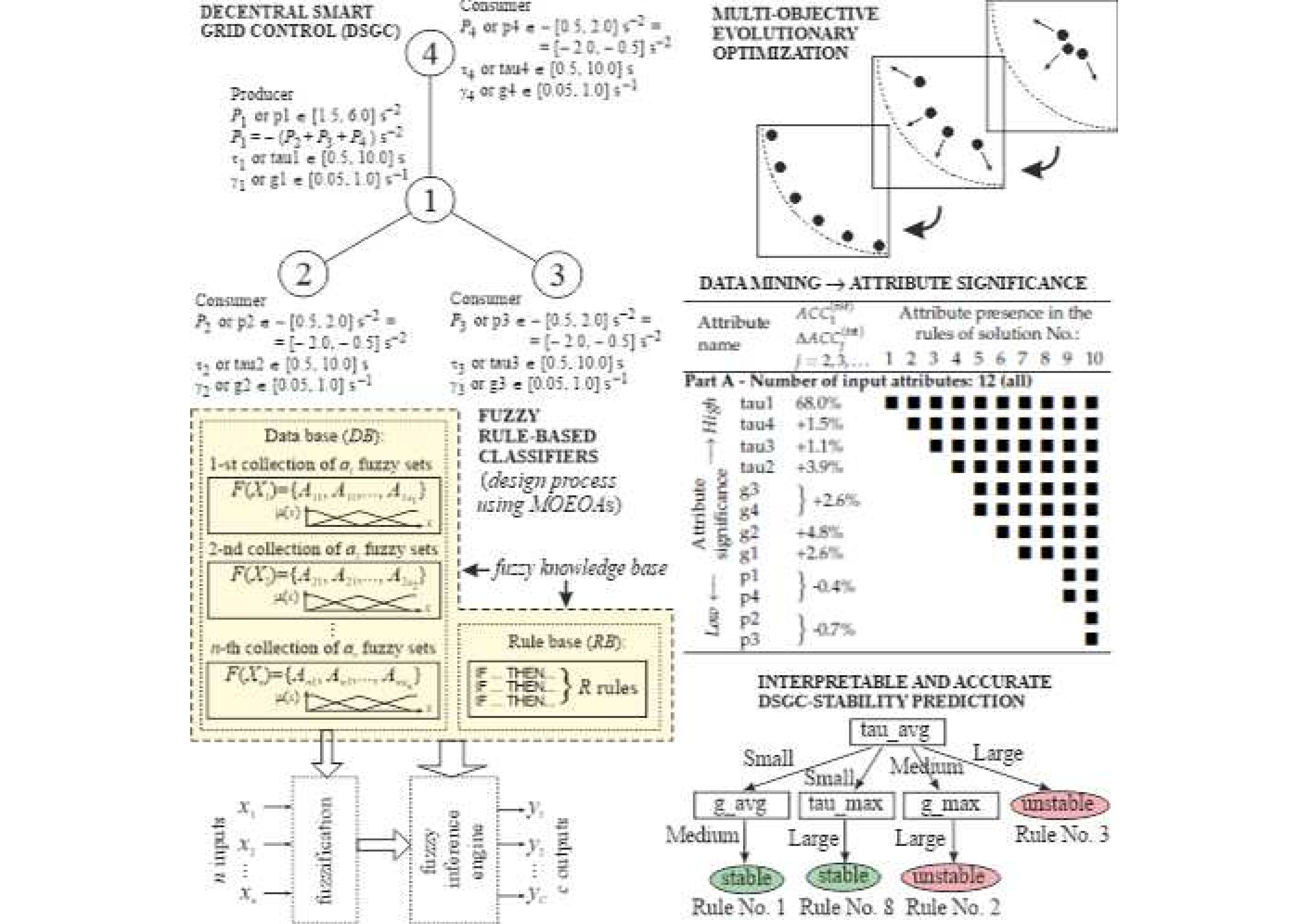
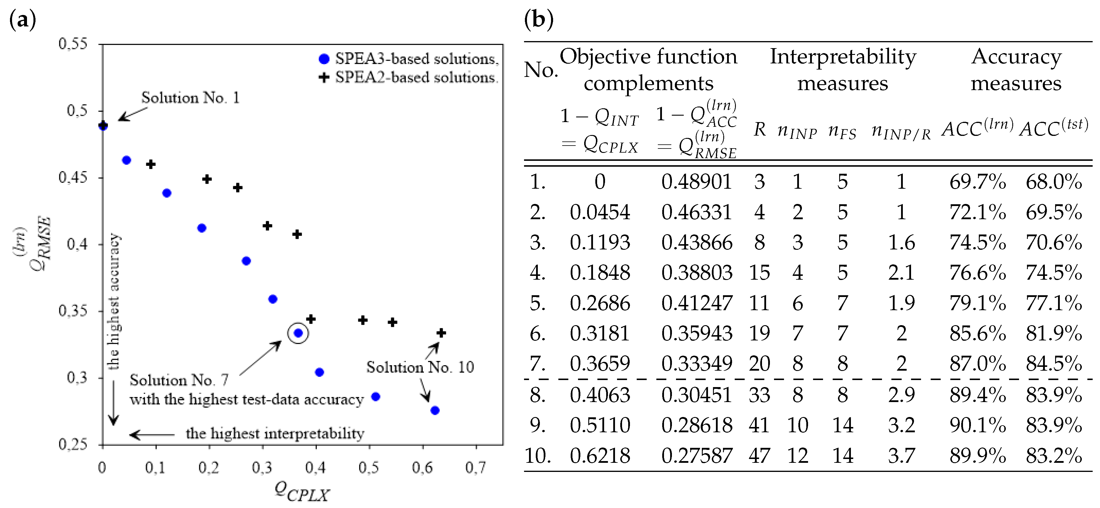
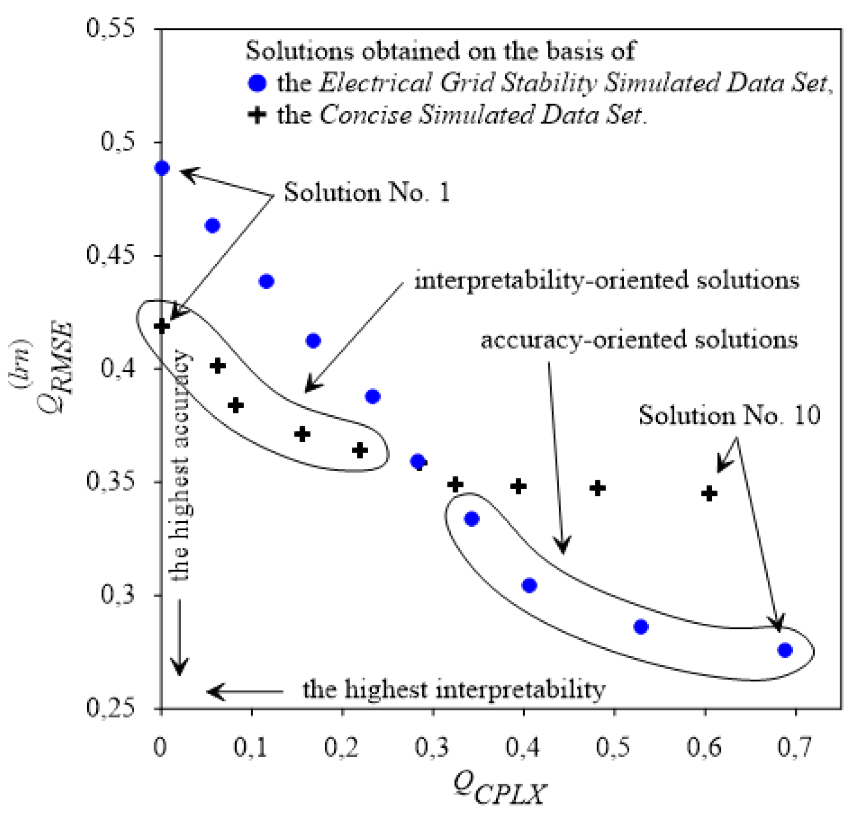
3. Electrical Grid Stability Simulated Data Set and Its Input-Aggregate-Based Version for Stability Prediction of a Four-Node Star System Implementing the DSGC Concept

As already mentioned in the Introduction of this paper, the Electrical Grid Stability Simulated Data Set available since November 2018 at the UCI Database Repository (https://archive.ics.uci.edu/ml) is the first set used in our experiments. This data set is the outcome of a simulation experiment using a two-part mathematical model of a four-node star grid implementing the DSGC concept. The first part of the model describes the physical dynamics of electric power generation and its connection with consumption loads. The second part is an economic structure which binds the electricity price to the grid frequency (see [11,13,14,19] for details). In the simulation experiment, three key input variables of the model were selected (each allowed to vary independently) for each of the four grid participants. These key input variables include: (i) $P_j$, $j=1,2,3,4$ (referred to as p1, ..., p4 in the simulated data set) describing the mechanical power produced (for $j=1$) or consumed (for $j=2,3,4$); (ii) ${\tau }_j$, $j=1,2,3,4$ (referred to as tau1, ..., tau4 in the simulated data set) describing reaction time of each grid participant to an electricity price change; and (iii) ${\gamma }_j$, $j=1,2,3,4$ (referred to as g1, ..., g4 in the simulated data set) which is a coefficient proportional to price elasticity for each grid participant. Figure 1 illustrates the structure of the DSGC system considered in the simulation experiment and the feasible solution space values (boundary conditions) for all the previously listed key input variables. Except for $P_1$ ($P_1=-(P_2+P_3+P_4)$ as shown in Figure 1), they all are sampled as uniform distributions throughout their respective feasible spaces to initialize and launch the simulations (10000 simulation runs were performed). Several other input variables of the two-part mathematical model of the DSGC system are kept unchanged during the simulation process. They include: (i) the averaging time T required to measure the price signal ($T=2s$), (ii) the coupling strength K proportional to line capacity ($K=8s^{-2}$), and (iii) the damping constant $\alpha$ ($\alpha =0.1s^{-1}$). The model’s output variable (referred to as stab in the simulated data set), i.e., the stability metric (ranging from −0.0808 to +0.1094), is quantified such that a negative value of that metric indicates that the grid is stable, whereas a positive value indicates that the grid is unstable. In the simulated data set the stab-variable is accompanied by a stabf label of the grid stability—a categorical attribute taking values from a two-element set: “stable” for stab < 0 and “unstable” for stab > 0. The details regarding the simulation experiment are presented in [14].

Therefore, the characteristics of the Electrical Grid Stability Simulated Data Set collecting the simulation experiment results and used in our experiments is the following. It contains 10,000 records (instances). Each record is characterized by 12 input attributes—tau1, tau2, tau3, tau4, p1, p2, p3, p4, g1, g2, g3, and g4; and two output attributes—stab and stabf, out of which only the stabf labels are used in our experiments (see

Table 1. Details of particular records of the Electrical Grid Stability Simulated Data Set used in our experiments.

No.	Attribute Name		Attribute Type	Attribute Domain Details				std.
					min.	max.	avg.	dev.
1.	input attributes	tau1	numerical	reaction time of electricity producer (in sec.)	0.50079	9.9995	5.25	2.7424
2.		tau2	numerical		0.50014	9.9998	5.25	2.7424
3.		tau3	numerical		0.50079	9.9995	5.25	2.7424
4.		tau4	numerical		0.50047	9.9994	5.25	2.7424
5.		p1	numerical	nominal power produced (positive values)	1.5826	5.8644	3.57	0.75212
6.		p2	numerical		−1.9999	−0.50011	−1.25	0.43301
7.		p3	numerical		−1.9999	−0.50007	−1.25	0.43301
8.		p4	numerical		−1.9999	−0.50002	−1.25	0.43301
9.		g1	numerical	gamma coefficient 1) for electricity producer	0.050009	0.99994	0.525	0.27424
10.		g2	numerical		0.050053	0.99994	0.525	0.27424
11.		g3	numerical		0.050054	0.99998	0.525	0.27424
12.		g4	numerical		0.050028	0.99993	0.525	0.27424
13.	output attr.	stab 2)	numerical	the maximal real part of the characteristic equation root (if positive—the system is linearly unstable)	−0.08076	0.1094	0.01573	0.03691
14.		stabf	categorical (class label)	2 class labels; class balance: “nstable” class (63.8% of all records) and “stable” class (36.2% of all records)

¹⁾ coefficient proportional to price elasticity; ²⁾ attribute “stab” is not used in our experiments.

for details).

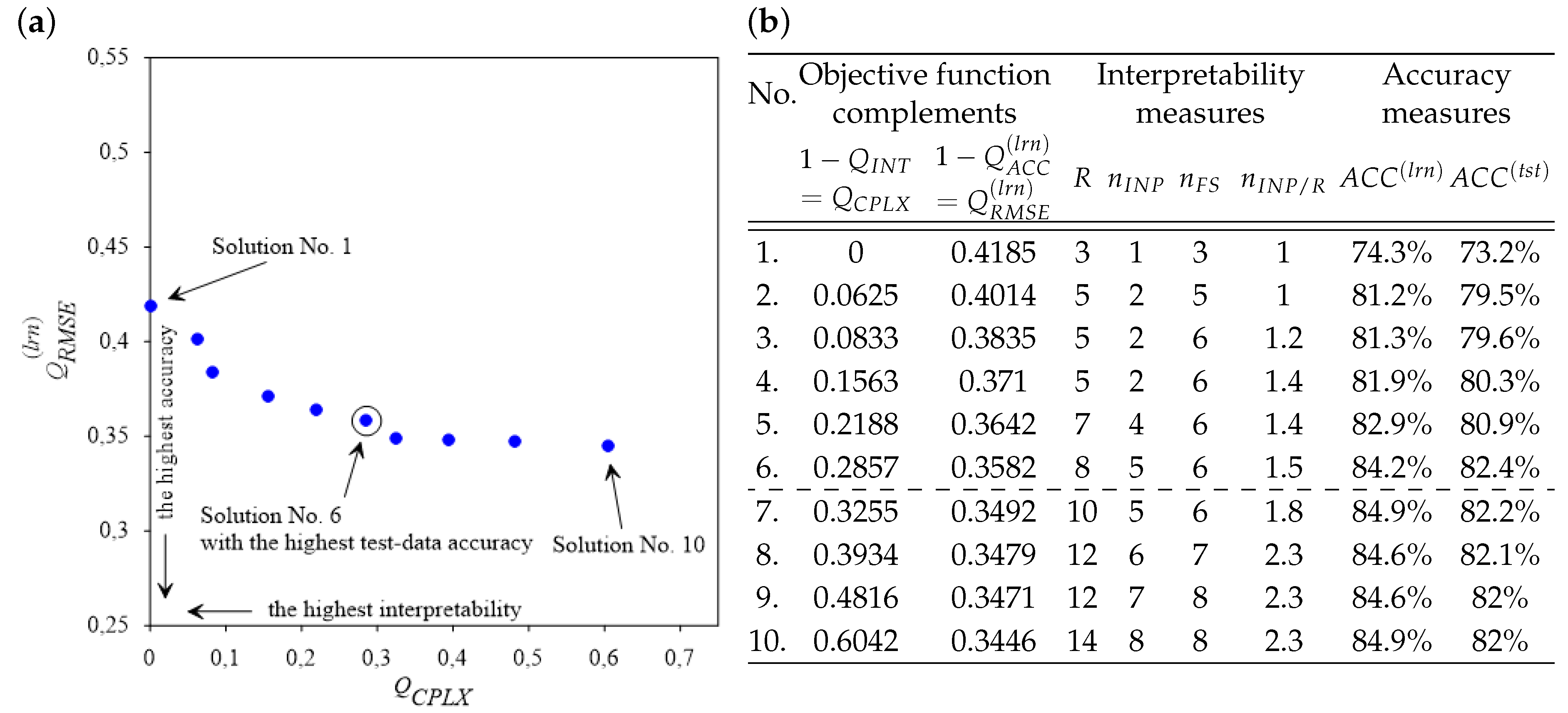
A more concise representation of the above-characterized simulated data set is proposed in [14]. It is based on aggregates—such as minimum, maximum, and average (mean) values—of input attributes across all grid participants. For instance, for the reaction time ${\tau }_j$, $j=1,\cdots ,4$, the input aggregates are the following: ${\tau }_{min}={min}_{j=1,\cdots ,4}{\tau }_j$, ${\tau }_{avg}=\frac{1}{4}{\sum }_{j=1}^4{\tau }_j$, and ${\tau }_{max}={max}_{j=1,\cdots ,4}{\tau }_j$. In the modified simulated data set, they are referred to as tau_min, tau_avg, and tau_max; analogously—p_min, p_avg, and p_max for $P_j$ and g_min, g_avg, and g_max for ${\gamma }_j$, $j=1,\cdots ,4$ (see

Table 2. Details of particular records of the input-aggregate-based version of the Electrical Grid Stability Simulated Data Set (referred to as the Concise Simulated Data Set) used in our experiment.

No.	Attribute Name		Attribute Type	Attribute Domain Details				std.
					min.	max.	avg.	dev.
1.	input attributes	tau_min	numerical		0.50014	8.874	2.4011	1.5649
2.		tau_avg	numerical		0.87644	9.446	5.25	1.3743
3.		tau_max	numerical		1.0217	9.9998	8.0944	1.5482
4.		p_min	numerical		0.5644	1.9999	1.6254	0.2913
5.		p_avg	numerical		0.5275	1.9548	1.25	0.2507
6.		p_max	numerical		1.5526	5.8644	3.75	0.7521
7.		g_min	numerical		0.05	0.8884	0.2397	0.1552
8.		g_avg	numerical		0.1194	0.9536	0.525	0.1369
9.		g_max	numerical		0.1459	0.9999	0.811	0.1539
10.	out. attr.	stabf	categorical (class label)	2 class labels; class balance: “unstable” class (63.8% of all records) and "stable" class (36.2% of all records)

¹⁾ coefficient proportional to price elasticity.

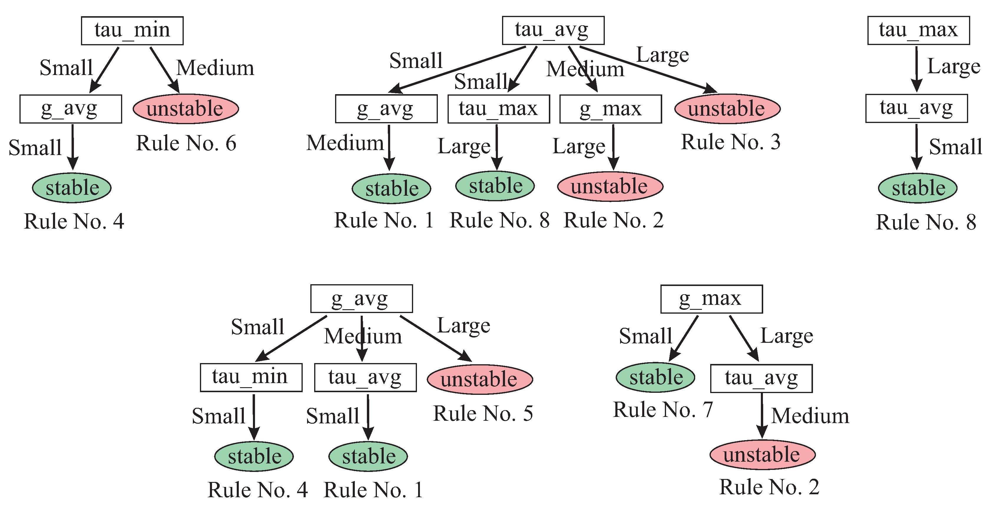
for details). The modified data set (referred to as the Concise Simulated Data Set) is the second set used in our experiments.

4. Methodology: Main Components of the Proposed FRBCs Designed from Data Using MOEOAs

In this section we briefly present the main components of our approach to designing FRBCs from data by means of MOEOAs. They are used to perform FRBCs’ learning and structure-and-parameter optimization, which also results in the optimization of FRBCs’ interpretability-accuracy trade-off (see [20,21,22,28] for details and discussion). The following components are characterized: learning data set, representation of input attributes and class labels, FRBC knowledge base, objectives of the FRBCs’ evolutionary optimization, original dedicated genetic operators introduced, and MOEOAs used in our experiments. An FRBC with n input attributes $x_1,x_2,\cdots ,x_n$ and an output—a fuzzy set over the set $Y=\{y_1,y_2,\cdots ,y_c\}$ of c class labels—is considered. Our approach can process both numerical and categorical attributes. However, in the DSGC-stability prediction problem, only numerical attributes occur. Hence, only numerical attributes will be considered from now on.

Learning data set L: The construction of the proposed FRBC is based on the data set L which contains K input–output samples:

$$\mathit{L}={\{{\mathit{x}}_k^{\left(lrn\right)},y_k^{\left(lrn\right)}\}}_{k=1}^K,$$

(1)

where ${\mathit{x}}_k^{\left(lrn\right)}=(x_{1k}^{\left(lrn\right)},x_{2k}^{\left(lrn\right)},\cdots ,x_{nk}^{\left(lrn\right)})\in \mathit{X}=X_1\times X_2\times \cdots \times X_n$ (× stands for Cartesian product of ordinary sets) represents the collection of input attributes and $y_k^{\left(lrn\right)}$ represents the corresponding class label ($y_k^{\left(lrn\right)}\in Y$) for the k-th data sample, $k=1,2,\cdots ,K$.

Representation of input attributes and class labels: Each numerical attribute $x_i$, $i\in \{1,2,\cdots ,n\}$ is represented by $a_i$ fuzzy sets $A_{i{k}_i}\in F\left(X_i\right)$, $k_i=1,2,\cdots ,a_i$, where $F\left(X_i\right)$ is a family of all fuzzy sets defined in the universe $X_i$, $i=1,2,\cdots ,n$. $A_{i1}$ represents an S-type fuzzy set (corresponding to linguistic term “Small”), $A_{i{a}_i}$ represents an L-type set (corresponding to linguistic term “Large”), and $A_{i2},A_{i3},\cdots ,A_{i,a_i-1}$ represent M-type sets (corresponding to linguistic terms “Medium 1,’ “Medium 2,’ ... , “Medium $a_i-2$”). For simplicity, $A_{i{k}_i}$s denote the corresponding linguistic terms also. 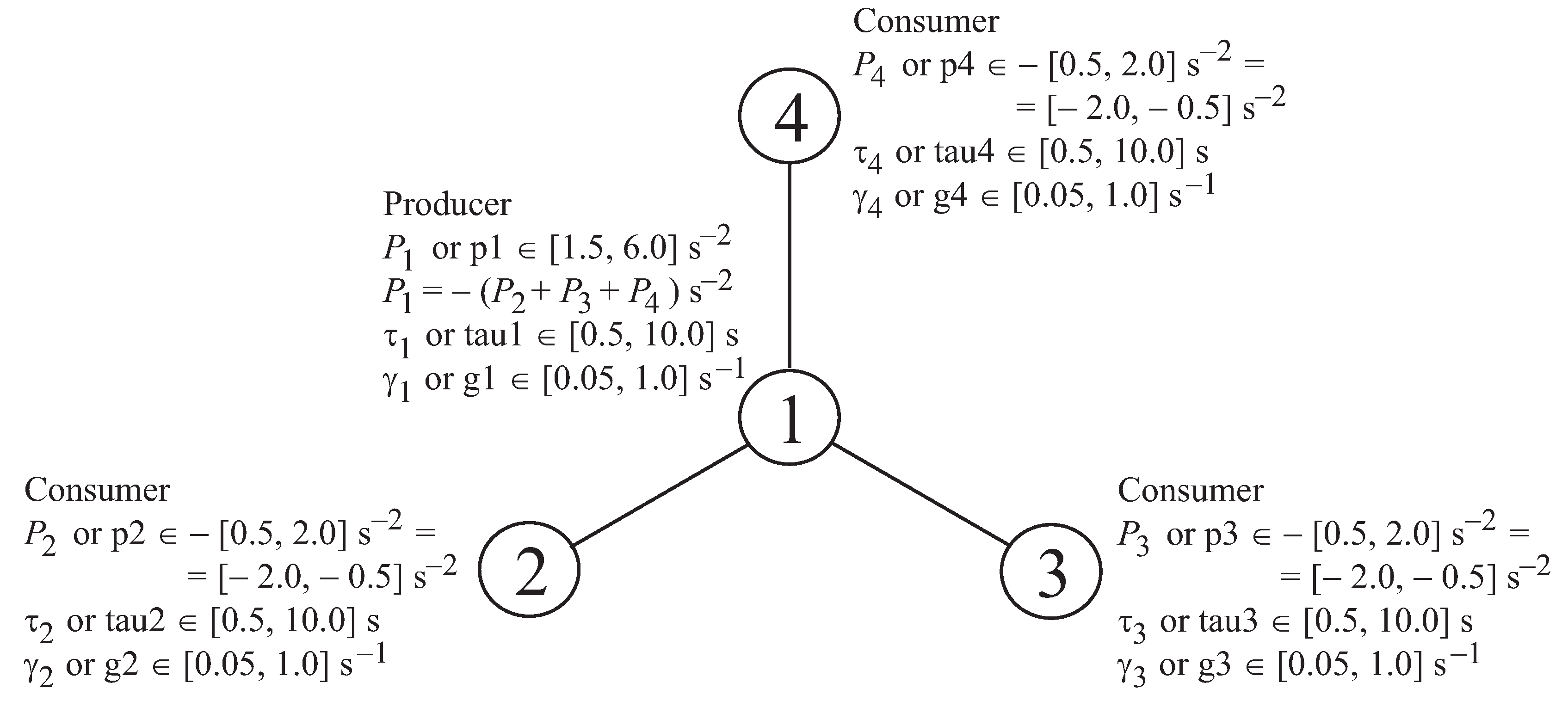Figure 2 shows trapezoidal membership functions for S, M, and L-type fuzzy sets used in our experiments. In turn, each class label $y_j$, $j\in \{1,2,\cdots ,c\}$ is represented by a fuzzy singleton $B_j=B_j^{(singl.)}$ with the following membership function: ${\mu }_{B_j^{(singl.)}}\left(y\right)=1$ for $y=y_j$ and 0 elsewhere.

FRBC’s knowledge base contains R genetically optimized fuzzy rules discovered in the learning data set (1). The form of the r-th rule, $r=1,2,\cdots ,R$, is the following (the overall number of rules R changes as the learning progresses):

$$\mathbf{IF}{[x_1\mathrm{is}{A}_{1,s{w}_1^{\left(r\right)}}]}_{(s{w}_1^{\left(r\right)}>0)}\mathbf{AND}\dots \mathbf{AND}{[x_n\mathrm{is}{A}_{n,s{w}_n^{\left(r\right)}}]}_{(s{w}_n^{\left(r\right)}>0)}\mathbf{THEN}y\mathrm{is}{B}_{j^{\left(r\right)}}^{(singl.)}.$$

(2)

Formula ${\left[expression\right]}_{\left(condition\right)}$ in (2) represents conditional inclusion of the $\left[expression\right]$-part into a given rule assuming that the ($condition$)-part is fulfilled. In turn, $s{w}_i^{\left(r\right)}$ denotes a switch-parameter which controls the presence/absence of the i-th input attribute in the r-th rule, $i=1,2,\cdots ,n$.

$s{w}_i^{\left(r\right)}\in \{0,1,2,\cdots ,a_i\}$, where $a_i$ is the number of fuzzy sets (and the corresponding linguistic terms) defined for the i-th attribute. For $s{w}_i^{\left(r\right)}=0$, the i-th attribute is removed from (not active in) that rule, whereas for $s{w}_i^{\left(r\right)}>0$ the component $\left[x_{i}is{A}_{i{k}_i}\right]$ ($k_i=s{w}_i^{\left(r\right)}$) is included (active) in that rule.

An FRBC’s knowledge base contains two separate modules; i.e., a rule-base-structure module RB and a data-base module DB. We propose a simple, direct, and thus computationally efficient RB representation as follows:

$$RB={\{s{w}_1^{\left(r\right)},s{w}_2^{\left(r\right)},\cdots ,s{w}_n^{\left(r\right)},j^{\left(r\right)}\}}_{r=1}^R.$$

(3)

In turn, DB contains tunable and non-tunable parts. The tunable part contains parameters of membership functions of fuzzy sets representing particular numerical input attributes. These parameters—subject to tuning during the FRBCs’ learning and MOEOA-based optimization—include (see Figure 2): $e_S$ and ${\rho }_S$ for S-type fuzzy sets; ${\sigma }_M$, $d_M$, $e_M$, and ${\rho }_M$ for M-type fuzzy sets; and ${\sigma }_L$ and $d_L$ for L-type fuzzy sets. The non-tunable part of DB contains the set of class labels $Y=\{y_1,y_2,\cdots ,y_c\}$.

Objectives of the FRBC’s evolutionary optimization: Two separate optimization objectives are considered; i.e., the accuracy and the interpretability of the system. The FRBC’s accuracy measure (subject to maximization) is defined as follows [20,21,22,40]:

$$Q_{ACC}^{\left(lrn\right)}=1-Q_{RMSE}^{\left(lrn\right)},$$

(4)

where

$$Q_{RMSE}^{\left(lrn\right)}=\sqrt{\frac{1}{Kc}\sum _{k=1}^K\sum _{j=1}^c{\left[{\mu }_{B_k^{(singl.)\left(lrn\right)}}\left(y_j\right)-{\mu }_{B_k^{\prime }}\left(y_j\right)\right]}^2}.$$

(5)

${\mu }_{B_k^{\prime }}\left(y\right)$ is the membership function of fuzzy set $B_k^{\prime }$, which is a response of system (2) for the learning data sample ${\mathit{x}}_k^{\left(lrn\right)}$. In turn, ${\mu }_{B_k^{(singl.)\left(lrn\right)}}\left(y\right)$ (equal to 1 for $y=y_k^{\left(lrn\right)}$ and to 0 elsewhere) is the membership function of fuzzy singleton $B_k^{(singl.)\left(lrn\right)}$, which is the desired fuzzy-singleton response for that sample ($Q_{RMSE}^{\left(lrn\right)}\in [0,1]$).

As far as the FRBC’s interpretability is concerned, we use the notion of interpretability in a broader sense, which includes two essential aspects; i.e., the FRBC’s complexity and semantic aspects of the FRBC’s operation. We evaluate the FRBC’s complexity-related interpretability using the following measure (subject to maximization):

$$Q_{INT}=1-Q_{CPLX},$$

(6)

where

$$Q_{CPLX}=\frac{Q_{RINP}+Q_{INP}+Q_{FS}}{3},$$

(7)

and

$$Q_{RINP}=\frac{1}{R}\sum _{r=1}^R\frac{n_{INP}^{\left(r\right)}-1}{n-1},Q_{INP}=\frac{n_{INP}-1}{n-1},Q_{FS}=\frac{n_{FS}-1}{{\sum }_{i=1}^n{a}_i-1},n>1.$$

(8)

The FRBC’s complexity measure $Q_{CPLX}$ (7) takes its values from interval [0, 1], where 0 represents the minimal complexity and 1 the maximal one. $Q_{CPLX}$ is an average of three sub-measures that evaluate: (i) an average complexity of particular rules $Q_{RINP}$ (8) ($n_{INP}^{\left(r\right)}$ in (8) denotes the number of active input attributes in the r-th rule); (ii) the complexity of the whole system in terms of its active inputs $Q_{INP}$ (8) ($n_{INP}$ in (8) denotes the number of active inputs in the whole system); and (iii) the whole-system complexity in terms of its active fuzzy sets $Q_{FS}$ (8) ($n_{FS}$ in (8) denotes the numbers of active fuzzy sets (linguistic terms) in the whole system).

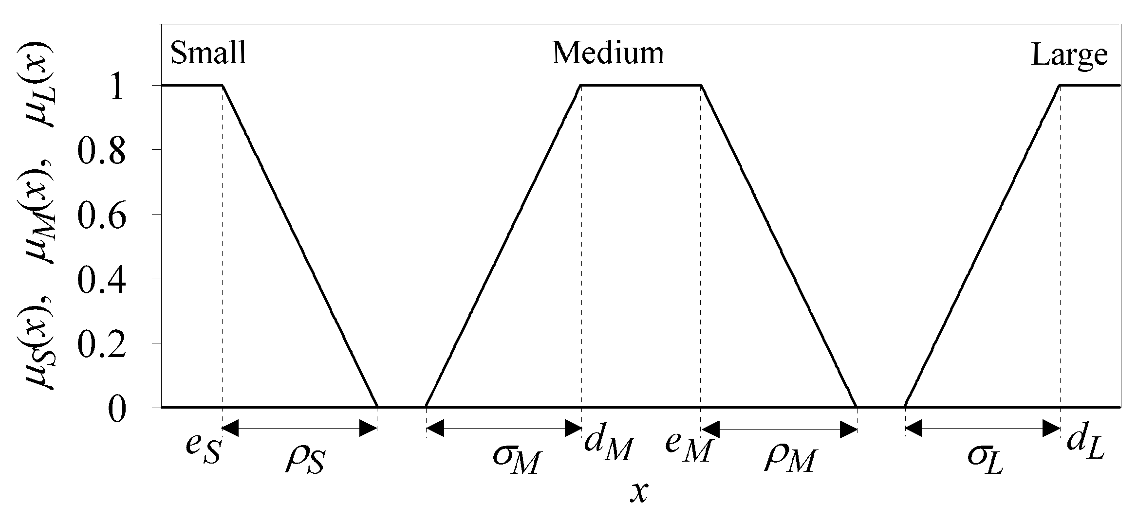
The FRBC’s semantics-related interpretability is addressed by us by imposing—as optimization constraints—the so-called strong fuzzy partitions (SFPs) [41] upon domains of particular numerical attributes. SFPs are special class of fuzzy partitions; namely, for any domain value, the sum of the values of all membership functions constituting SFP is equal to 1. It can be shown [41] that SFPs satisfy the desired demands regarding the semantics-related interpretability. Straightforward implementation of SFP requirements for the case of trapezoidal membership functions can be formulated in the following way (see Figure 3 for illustration of the SFP-requirements’ implementation for the three-set SFP of $x_i$-domain):

$${\sigma }_{i{k}_i}={\rho }_{i,k_i-1}=d_{i{k}_i}-e_{i,k_i-1},k_i=2,3,\cdots ,a_i$$

(9)

and, obviously,

$$e_{i1}\le d_{i2}\le e_{i2}\le \cdots \le d_{i,a_i-1}\le e_{i,a_i-1}\le d_{i{a}_i},i=1,2,\cdots ,n.$$

(10)

Original, dedicated genetic operators introduced: A population of FRBC’s knowledge bases (each represented by its RB and DB) is processed during the genetic learning process. We developed original crossover and mutation operators for the transformation of the RB population. The crossover operator processes two individuals (i.e., two RBs) containing $R_1$ and $R_2$ fuzzy rules, respectively, by performing one sub-operation randomly selected from the set of five sub-operations referred to as Cro-RB1, Cro-RB2, ..., Cro-RB5. They are defined as follows:

Cro-RB1 (labeled as “exchange of many fuzzy rules”) operates in two stages. First, for the r-th rule in both RBs, $r=1,2,\cdots ,min(R_1,R_2)$, a random-switch condition (equivalent to the random selection of 1 from the set {0, 1}) is checked. Then, the r-th rules from both RBs are exchanged, provided that the random-switch condition is fulfilled. Second, each of the remaining rules of the larger RB is moved to the smaller RB, provided that its random-switch condition is fulfilled.

Cro-RB2 (labeled as “exchange of a single fuzzy rule”) is similar to Cro-RB1 but the Cro-RB1 activities are carried out unconditionally and only once for randomly selected single rule from the larger RB.

Cro-RB3 (labeled as “exchange of many fuzzy sets in many fuzzy rules”) is analogous to the first stage of Cro-RB1. This time, the random-switch condition is run for each input attribute and for the output class label from the corresponding rules coming from both RBs. Fuzzy sets describing a given input attribute or class label in both RBs are exchanged provided that their random-switch conditions are fulfilled.

Cro-RB4 (labeled as “exchange of many fuzzy sets in a single fuzzy rule”) performs the activities of Cro-RB3 unconditionally and only once for a randomly selected single rule from the first RB and its counterpart from the second RB.

Cro-RB5 (labeled as “exchange of a single fuzzy set”) is a special case of Cro-RB4. The activities of Cro-RB4 are performed unconditionally and only once for a randomly selected input attribute or output class label.

The mutation operator for the RB transformation processes a single individual (i.e., a single RB) by performing one sub-operation randomly selected from the set of four sub-operations referred to as Mut-RB1, Mut-RB2, Mut-RB3, Mut-RB4. They are defined as follows:

Mut-RB1 (labeled as “fuzzy rule insertion”) inserts into RB a new fuzzy rule (2) with randomly selected values of switches $s{w}_i^{\left(r\right)}$ ($s{w}_i^{\left(r\right)}\in \{0,1,2,\cdots ,a_i\}$, $i=1,2,\cdots ,n$) and class label $j^{\left(r\right)}$ ($j^{\left(r\right)}\in \{1,2,\cdots ,c\}$).

Mut-RB2 (labeled as “fuzzy rule deletion”) removes a randomly selected fuzzy rule from the RB.

Mut-RB3 (labeled as “change a single fuzzy set”) randomly selects one fuzzy rule from the RB and its one i-th input attribute or output class label j. Next, it randomly selects a new value of its switch $s{w}_i$ or class label j.

Mut-RB4 (labeled as “change of an input in a fuzzy rule”) randomly selects: (i) one fuzzy rule from the RB, (ii) its one active input attribute (i.e., with $s{w}_{i_1}>0$), and (iii) its one non-active input attribute (i.e., with $s{w}_{i_2}=0$). Then, the first attribute is set to be non-active (i.e., $s{w}_{i_1}=0$) and the second attribute—to be active (i.e., $s{w}_{i_2}>0$) in that rule.

The crossover and mutation operators for the RB-population transformation are followed by three RB-repairing operators. The first operator removes “empty” fuzzy rules, i.e., the rules with all non-active input attributes (with $s{w}_i=0$ for $i=1,2,\cdots ,n$), whereas the second one removes rule duplicates. In turn, the third operator adds—for each class label that is currently not represented in RB—one fuzzy rule with that class label (in order to preserve the principle “at least one fuzzy rule per class in RB”).

DB population transformation is performed by means of separate genetic operators. The crossover operator (processing two individuals; i.e., two DBs), randomly selects one fuzzy set from each DB. New values of d and e-parameters, which characterize membership functions of both fuzzy sets (see Figure 2) are calculated as linear combinations of their old values from both sets; they also must fulfill condition (10). New values of $\sigma$ and $\rho$-parameters are calculated from (9) using new values of d and e-parameters. The mutation operator (processing a single individual, i.e., a single DB) randomly selects one fuzzy set from the DB and one of its two parameters d and e (say, d is selected). Its new value $d_{new}=d+rand(-0.2,0.2)[x_{i,max}-x_{i,min}]$, where $rand(·)$ returns a random number from the assumed interval and $[x_{i,min},x_{i,max}]$ is a range of the domain of the selected set. New values of $\sigma$ and $\rho$-parameters are calculated from (9).

MOEOAs used in our experiments: The performances of different MOEOAs are usually evaluated and compared in terms of three aspects [42]. First, the accuracy of generated non-dominated solutions is considered. The accuracy represents the closeness of those solutions to either the Pareto-optimal solutions, or if they are not available, to reference solutions. Second, the spread of the solution set is investigated; i.e., how well these solutions arrive at the extrema of the Pareto-optimal or reference solution sets. The spread is usually represented by the distance between the extreme solutions in the set. Third, the distribution of the solutions in the set, i.e., how evenly distributed they are along the approximation of Pareto-optimal front in the objective space, is considered. A set of solutions which are more accurate and are characterized by a higher spread and a better-balanced distribution outperforms the alternative solution sets.

For the purpose of comparison, two MOEOAs are used in experiments reported in this work; i.e., the well-known SPEA2 method and our generalization of SPEA2, referred to as SPEA3. In comparison with SPEA2, the proposed SPEA3 approach generates sets of non-dominated solutions characterized by higher spread and a more even distribution in the objective space. The essence of the proposed SPEA2’s generalization consists of replacing its environmental selection procedure with our original algorithm, which improves both the spread and distribution balance of generated solutions. The environmental selection consists of selecting a representation of the best solutions from all solutions obtained so far and keeping them in an external archive of a fixed size. In SPEA2 all non-dominated solutions from the archive and the current population are copied to the next-generation archive (to fill the archive, the best dominated solutions are copied to it). In the case of overfilling the archive, a truncation procedure is run to reduce the archive size to the predefined level. Thus, only the truncation procedure (if activated) contributes to improving the distribution balance and diversity of the final set of solutions. On the contrary, the proposed environmental selection algorithm implemented in SPEA3 is fully-oriented towards achieving these goals. The archive is iteratively increased by gradual adding of carefully selected non-dominated solutions from the current population (in each subsequent generation, a single solution characterized by possible longest and similar distances to its near neighbors is added). Then, a process of relocation of particular archived solutions aiming at increasing average distances between solutions and their nearest neighbors is carried out. Said relocation is performed by gradual replacement of archived solutions by new solutions selected from the population in such a way as (i) to maximize the distances between extreme solutions (which results in improving the spread of solutions) and (ii) to minimize the distance differences between neighboring solutions (which results in improving the distribution of solutions). Concluding, in our approach, the complementary operations of increasing and reducing the archive aim at obtaining the best available distribution balance and spread of solutions belonging to Pareto-front approximation (see [28,29] for detailed presentation and discussion).

5. Experiments (Application of Our Approach to DSGC-Stability Prediction) and Discussion

In this section we present the results of two experiments (for both data sets characterized in Section 3 of this paper) regarding the application of our approach to interpretable and accurate DSGC-stability prediction.

5.1. Application to Electrical Grid Stability Simulated Data Set

We start with revealing some details of the operation of our method for constructing FRBCs from the considered simulated data set. Figure 4a presents two 10-element-collections of non-dominated solutions (optimized FRBCs) generated in a single run of our FRBCs’ design technique employing, independently, our SPEA3 and SPEA2 algorithms. Both experiments of genetic learning have been performed for a learning-test data split with 1:9 ratio. It means that only 10% of the whole original data set (preserving the class proportions) is used as the learning data to construct the system, whereas the remaining 90% of the original data are used for the system’s testing. It is worth emphasizing that such a data split poses a significant challenge to any system’s design technique. Each collection of solutions of Figure 4a represents the best available approximations of Pareto-optimal solutions generated either by our SPEA3 or SPEA2. Particular solutions from a given collection (front) are characterized by different levels of optimized interpretability-accuracy trade-off. Thus, the user can select a single solution (a specific FRBC) with a desired degree of compromise between the interpretability and accuracy.

Figure 4a shows that our SPEA3-based approach generates the collection of solutions characterized by: (i) a much-better-balanced distribution in the objective space (i.e., the solutions are distributed along the front in a much more even way) and (ii) higher accuracy (i.e., the closeness to Pareto-optimal front). Therefore, our SPEA3-based approach outperforms its SPEA2-based counterpart (see Section 4 of this paper for MOEOAs’ performance evaluation criteria). The interpretability and accuracy-related numerical details of all SPEA3-based solutions (FRBCs) from Figure 4a are collected in Figure 4b, in which $n_{INP/R}$ is the number of input attributes per rule, whereas $AC{C}^{\left(lrn\right)}$ is the percentage of correct decisions in the learning set and $AC{C}^{\left(tst\right)}$—in the test set (the remaining parameters were defined in Section 4 of the paper).

Fuzzy rule bases of exemplary SPEA3-based solutions (FRBCs) are presented in

Table 3. Fuzzy rule bases for SPEA3-based solutions (FRBCs) 1–3 from Figure 4.

No.	Fuzzy Classification Rules
Solution No. 1 ($AC{C}^{\left(tst\right)}=68\%$):
1.	IF	tau1 is Small THEN stable
2.	IF	tau1 is Medium THEN unstable
3.	IF	tau1 is Large THEN unstable
Solution No. 2 ($AC{C}^{\left(tst\right)}=69.5\%$):
1–3.	These rules are the same as rules 1–3 from Solution No. 1.
4.	IF	tau4 is Small THEN stable
Solution No. 3 ($AC{C}^{\left(tst\right)}=70.6\%$):
1,2.	These rules are the same as rules 1, 2 from Solution No. 2.
3.	IF	tau1 is Large AND tau4 is Medium THEN unstable
4.	This rule is the same as rule 4 from Solution No. 2.
5.	IF	tau1 is Large AND tau4 is Large THEN unstable
6.	IF	tau3 is Small AND tau4 is Medium THEN stable
7.	IF	tau3 is Medium AND tau4 is Medium THEN unstable
8.	IF	tau3 is Large AND tau4 is Large THEN unstable

and

Table 4. Fuzzy rule base for SPEA3-based solution (FRBC) 7 from Figure 4 which is characterized by the highest test-data accuracy.

No.	Fuzzy Classification Rules
Solution No. 7 ($AC{C}^{\left(tst\right)}=84.5\%$):
1.	IF	tau1 is Small AND tau2 is Small THEN stable
2.	IF	tau1 is Small AND tau3 is Small THEN stable
3.	IF	tau1 is Small AND tau4 is Small THEN stable
4.	IF	tau1 is Small AND g2 is Small THEN stable
5.	IF	tau1 is Small AND g4 is Small THEN stable
6.	IF	tau1 is Medium AND g4 is Large THEN unstable
7.	IF	tau1 is Large AND g1 is Large THEN unstable
8.	IF	tau2 is Small AND tau3 is Small THEN stable
9.	IF	tau2 is Small AND tau4 is Small THEN stable
10.	IF	tau2 is Small AND g3 is Small THEN stable
11.	IF	tau2 is Medium AND g2 is Large THEN unstable
12.	IF	tau2 is Large AND g2 is Large THEN unstable
13.	IF	tau3 is Small AND tau4 is Small THEN stable
14.	IF	tau3 is Small AND g4 is Small THEN stable
15.	IF	tau3 is Large AND g3 is Large THEN unstable
16.	IF	tau4 is Small AND g3 is Small THEN stable
17.	IF	tau4 is Large AND g4 is Large THEN unstable
18.	IF	g1 is Small AND g2 is Small THEN stable
19.	IF	g1 is Small AND g2 is Medium AND g4 is Medium THEN stable
20.	IF	g2 is Small AND g3 is Small THEN stable

(membership functions of fuzzy sets representing input attributes used are also included). Table 4 presents the fuzzy rule base for the SPEA3-based solution (FRBC) 7 from Figure 4 which is characterized by the highest test-data accuracy. In turn, Table 3 reveals an interesting regularity, i.e., the fuzzy rule base of the solution 2 contains three rules from the solution 1. In turn, the fuzzy rule base of the solution 3 contains three rules from the solution 2, etc. Therefore, if higher system accuracy is required, then our approach adds some additional fuzzy rules (or extends the earlier-discovered rules) to provide a more detailed, and thus, more accurate description of the considered prediction problem. Said regularity confirms the internal integrity of our approach. This regularity is also illustrated in

Table 5. Illustration of attribute presence and significance in the Electrical Grid Stability Simulated Data Set.

Attribute Name		${ACC}_1^{\left(\mathrm{tst}\right)}$ $\Delta {ACC}_{\mathit{j}}^{\left(\mathrm{tst}\right)}$ $\mathit{j}=2,3,\cdots$	Attribute Presence in the
			Rules of Solution No.:
			1	2	3	4	5	6	7	8	9	10
Part A—Number of input attributes: 12 (all)
Low⟵Attribute significance⟶High	tau1	68.0%	■	■	■	■	■	■	■	■	■	■
	tau4	+1.5%		■	■	■	■	■	■	■	■	■
	tau3	+1.1%			■	■	■	■	■	■	■	■
	tau2	+3.9%				■	■	■	■	■	■	■
	g3	} +2.6%					■	■	■	■	■	■
	g4						■	■	■	■	■	■
	g2	+4.8%						■	■	■	■	■
	g1	+2.6%							■	■	■	■
	p1	} −0.4%									■	■
	p4										■	■
	p2	} −0.7%										■
	p3											■
Part B—Number of input attributes: 11
Low⟵Attribute significance⟶High	tau1—removed attribute
	tau4	67.7%	■	■	■	■	■	■	■	■	■	■
	tau3	+0.7%		■	■	■	■	■	■	■	■	■
	tau2	+2.0%			■	■	■	■	■	■	■	■
	g3	+2.2%				■	■	■	■	■	■	■
	g4	+3.4%					■	■	■	■	■	■
	g2	+3.9%						■	■	■	■	■
	g1	+1.8%								■	■	■
	p2	} −0.6%									■	■
	p4										■	■
	p3	} +0.2%										■
	p1											■
Part C—Number of input attributes: 10
Low⟵Attribute significance⟶High	tau1
	tau4
	tau3	66.1%	■	■	■	■	■	■	■	■	■	■
	tau2	+2.2%		■	■	■	■	■	■	■	■	■
	g3	+2.4%				■	■	■	■	■	■	■
	g2	+3.0%					■	■	■	■	■	■
	g4	+2.5%						■	■	■	■	■
	g1	+3.7%							■	■	■	■
	p1	+0.3%								■	■	■
	p3	−0.2%									■	■
	p2	} −0.1%										■
	p4											■
Part D—Number of input attributes: 9
Low⟵Attribute significance⟶High	tau1
	tau4
	tau3
	tau2	66%	■	■	■	■	■	■	■	■	■	■
	g4	+2.6%		■	■	■	■	■	■	■	■	■
	g3	+1.7%				■	■	■	■	■	■	■
	g2	+2.8%						■	■	■	■	■
	g1	+1.4%							■	■	■	■
	p1	−0.3%								■	■	■
	p2	} −0.8%									■	■
	p3										■	■
	p4	−2.4%										■
Part E—Number of input attributes: 8
Low⟵Attribute significance⟶High	tau1
	tau4
	tau3
	tau2
	g3	64%	■	■	■	■	■	■	■	■	■	■
	g2	+3.6%		■	■	■	■	■	■	■	■	■
	g1	+0.6%				■	■	■	■	■	■	■
	g4	+2.2%					■	■	■	■	■	■
	p3	−0.1%							■	■	■	■
	p2	−0.5%								■	■	■
	p1	0.0%									■	■
	p4	−0.2%										■
Part F—Number of input attributes: 7
Low⟵Attribute significance⟶High	tau1
	tau4
	tau3
	tau2
	g3
	g2	+62.7%	■	■	■	■	■	■	■	■	■	■
	g4	+5.1%		■	■	■	■	■	■	■	■	■
	p1	−3.1%					■	■	■	■	■	■
	g1	+3.1%						■	■	■	■	■
	p4	−1.9%								■	■	■
	p3	+0.6%									■	■
	p2	+0.8%										■
Part G—Number of input attributes: 6
Low⟵Attribute significance⟶High	tau1
	tau4
	tau3
	tau2
	g3
	g2
	g4	62.2%	■	■	■	■	■	■	■	■	■	■
	p1	+1.3%		■	■	■	■	■	■	■	■	■
	g1	+1.6%					■	■	■	■	■	■
	p2	+0.1%								■	■	■
	p4	+0.3%									■	■
	p3	−0.6%										■
Part H—Number of input attributes: 5
Low⟵Attribute significance⟶High	tau1
	tau4
	tau3
	tau2
	g3
	g2
	g4
	g1	62.1%	■	■	■	■	■	■	■	■	■	■
	p1	+1.1%		■	■	■	■	■	■	■	■	■
	p2	0.0%						■	■	■	■	■
	p4	−0.1%								■	■	■
	p3	−0.1%									■	■

(see, first, Part A of Table 5) in which each black square denotes the presence of a given input attribute in the fuzzy rule base of a given solution (FRBC). $AC{C}_1^{\left(tst\right)}$ is the test-data accuracy of the system exclusively based on the most significant input attribute. In Part A of Table 5 the most significant attribute is tau1, occurring in the solution 1 and giving $AC{C}_1^{\left(tst\right)}=68\%$. Moreover, $\Delta AC{C}_j^{\left(tst\right)}$, $j=2,3,\cdots$ is the accuracy increase following the inclusion of the 2nd, 3rd, ⋯ most significant attributes into the system. In Part A of Table 5, the inclusion of tau4 (2nd most significant attribute) yields 1.5% increase in the test-data-accuracy and is related to the solution 2. In turn, the inclusion of tau3 (3rd most significant attribute) gives a further 1.1% test-data-accuracy-increase and is related to the solution 3, etc.

In such a way, we can uncover the hierarchy of significance of particular attributes. However, the obtained attribute-significance hierarchy is correct provided that no “overlapping” of some input attributes over the other ones occurs in the simulated data set. In order to verify that, we remove from the original data set the so-far most significant attribute, i.e., tau1, and we repeat, in an analogous way, the learning experiment. Its results are presented in Part B of Table 5, giving tau4 attribute the most significance place. Tau4 occupied second position in the experiment of Part A. Therefore, we conclude that tau4 is not "overlapped" by tau1. In the next step, we remove tau4 from the present data set and repeat the learning experiment—see Part C of Table 5—obtaining tau3 as the most significant attribute at this stage. It occupied second position in experiment of Part B. Therefore, tau3 is not “overlapped” by tau4. We repeat analogous experiments several times; i.e., we remove the most significant—at a given stage—input attribute and repeat the learning process on the reduced data set—see Parts D–H of Table 5. In such a way, we arrive to the real final hierarchy of input attribute significance in the DSGC-stability prediction problem. It is shown in the left part of

Table 6. Final hierarchy of attribute significance—a comparison of our approach and an alternative method of [43] (Electrical Grid Stability Simulated Data Set).

	Our Approach		Alternative Approach of [43] (Panda and Das (2019))
	Attribute Name	${ACC}_1^{\left(tst\right)}$	Attribute Name	Importance
Attribute significance Low⟵ ⟶High	tau1	68.2%	tau2	0.064
	tau4	67.8%	tau4	0.061
	tau3	66%	tau3	0.06
	tau2	66%	tau1	0.058
	g3	64%	g3	0.057
	g2	62.7%	g2	0.05
	g4	62.2%	g4	0.044
	g1	62.1%	g1	0.041
	p1, p2, p3, and p4 1)	-	p1, p2, p3, and p4	≪ 0.001

¹⁾ The attributes p1, p2, p3, and p4 do not occur in the fuzzy rule base of our most accurate solution 7 (see Table 4) and have not been tested.

that $AC{C}_1^{\left(tst\right)}$ has the same meaning as in Table 5; i.e., it is the test-data-accuracy of the system exclusively based on a single attribute listed to the left of $AC{C}_1^{\left(tst\right)}$ in Table 6.

The results of an alternative approach addressing the hierarchy of importance of particular input attributes in the considered simulated data set and proposed in [43] are presented in the right part of Table 6. The following remarks are formulated in [43]: “The time response of the consumers and producer to the price fluctuation play a more important role in the grid stability, as compared to the price elasticity index... Unstable grid conditions generally prevail for higher values of $\tau$ and $\gamma$...The power consumption pattern does not show any difference under stable and unstable grid conditions thus conforming with the analysis of feature selection obtained.” (a quote from [43]). The results of our experiments are consistent with all the above comments.

The cross-validation experiment with 1:9 learning-test data split ratio is the next and important part of our work. Each single learning experiment begins with generation of a Pareto-front approximation. Next, a single solution with, first, the highest test-data accuracy, and second, the highest interpretability, is chosen from that front approximation. In turn, the results from all partial experiments are averaged. The experiment is then repeated 10 times for different initializations of our approach. The averaged results are shown in the last row of

Table 7. Results of our approach and comparison with alternative methods for the Electrical Grid Stability Simulated Data Set.

Source		Method	Learn-to- Test Ratio	Number of Runs	Average Accuracy Measures for Learning and Test Data		Average Interpretability Measures
					$\overline{{ACC}^{\left(lrn\right)}}$	$\overline{{ACC}^{\left(tst\right)}}$	$\overline{\mathit{R}}$	${\overline{\mathit{n}}}_{ATR}$	${\overline{\mathit{n}}}_{FS}$	${\overline{\mathit{n}}}_{ATR/\mathit{R}}$
[44] (Moldovan and Salomie (2019))		-	n/a	63.9%	n/a	-	10	-	-
		-	n/a	87.8%	n/a	n/a	10	n/a	n/a
		-	n/a	88%	n/a	n/a	10	n/a	n/a
		-	n/a	91.9%	n/a	-	10	-	-
		-	n/a	66.3%	n/a	-	102	-	-
		-	n/a	83.7%	n/a	n/a	102	n/a	n/a
		-	n/a	88.8%	n/a	n/a	102	n/a	n/a
		-	n/a	91.5%	n/a	-	102	-	-
		-	n/a	64.7%	n/a	-	111	-	-
		-	n/a	84.3%	n/a	n/a	111	n/a	n/a
		-	n/a	87%	n/a	n/a	111	n/a	n/a
		-	n/a	93.8%	n/a	-	111	-	-
[45] (Karim (2019))	kNN	n/a	n/a	80.4%	n/a	-	12	-	-
	SVM	n/a	n/a	82.2%	n/a	-	12	-	-
	RBF	n/a	n/a	62.7%	n/a	-	12	-	-
	Decision Tree	n/a	n/a	84%	n/a	n/a	12	n/a	n/a
	RF	n/a	n/a	88.5%	n/a	n/a	12	n/a	n/a
	Naive Bayes	n/a	n/a	83.6%	n/a	-	12	-	-
	QDA	n/a	n/a	82.7%	n/a	-	12	-	-
[46] (Balali et al. (2020))	Fine Tree	n/a	n/a	84.2%	n/a	n/a	12	n/a	n/a
	Bagged Tree	n/a	n/a	91.5%	n/a	n/a	12	n/a	n/a
	Fine KNN	n/a	n/a	81.1%	n/a	-	12	-	-
	Weighted KNN	n/a	n/a	86.6%	n/a	-	12	-	-
	LR	n/a	n/a	81.5%	n/a	-	12	-	-
	Linear SVM	n/a	n/a	81.5%	n/a	-	12	-	-
	Quadratic SVM	n/a	n/a	94.2%	n/a	-	12	-	-
	Cubic SVM	n/a	n/a	96.9%	n/a	-	12	-	-
[47] (Chen, Chan, Wu and Lam (2019))		4:1	50	n/a	87.55%	-	12	-	-
		4:1	50	n/a	87.68%	-	12	-	-
		4:1	50	n/a	86.72%	-	12	-	-
		4:1	50	n/a	86.72%	-	12	-	-
		4:1	50	n/a	86.72%	-	12	-	-
		4:1	50	n/a	52.69%	-	12	-	-
		4:1	50	n/a	87.56%	-	12	-	-
		4:1	50	n/a	87.67%	-	12	-	-
		4:1	50	n/a	87.27%	-	12	-	-
		4:1	50	n/a	87.27%	-	12	-	-
		4:1	50	n/a	87.27%	-	12	-	-
		4:1	50	n/a	64.53%	-	12	-	-
This paper		Our approach based on SPEA3	1:9	10	91.1%	85.5%	22.7	9.7	26.9	4.1

n/a stands for not available.

, which also collects the results of as many as 39 alternative approaches applied to the considered data set; i.e., the Electrical Grid Stability Simulated Data Set. There are four groups of them. The first one, considered in [44], includes four methods: logistic regression (LR), random forest (RF), gradient boosted trees (GBT), and multilayer perceptron classifier (MPC). Each of them was supported, independently, by three feature selection algorithms: multivariate adaptive regression splines (MARS) algorithm, binary kangaroo mob optimization feature selection (BKMOFS) algorithm, and binary particle swarm optimization feature selection (BPSOFS) algorithm. The second group, considered in [45], includes seven methods: k-nearest neighbors (kNN) algorithm, support vector machine (SVM), radial basis function (RBF) network, decision trees, RF, naive Bayes approach, and quadratic discriminant analysis (QDA). The third group, considered in [46], includes eight methods: fine and bagged-tree algorithms, fine and weighted-kNN, LR, and linear, quadratic, and cubic-SVMs. The last group, considered in [47], includes six methods: the stochastic damped regularized LBFGS algorithm (Sd-REG-LBFGS; LBFGS stands for the limited memory Broyden–Fletcher–Goldfarb–Shanno algorithm), stochastic damped regularized LBFGS without regularization (SdLBFGS), robust stochastic approximation (RSA), stochastic approximation averaging (SAA), stochastic gradient difference (SGD), and a method of gradient-based stochastic optimization (Adam [48]). Each of them was used, independently, with logistic regression and Bayesian logistic regression algorithms.

The overwhelming majority of the alternative approaches of Table 7 are the black-box methods focused only on the system’s accuracy. Moreover, for methods applied in [44,45,46] only the learning-data-accuracy is available. Therefore, it is not possible to assess their generalizing capabilities (usually measured by test-data-accuracy), which belong to essential performance-evaluation criteria of any system designed from data. Some of the methods of [44] operate on more than 100 features, whereas the remaining approaches typically use 12 attributes; i.e., all the input attributes from the simulated data set. The experiments of [47] are performed for the 4:1 learning-test data split ratio, which significantly favors them in regard to our experiments using only 1:9 learning-test data split ratio. Despite that, our approach provides not only comparable test-data accuracy but also a detailed insight—in the form of fuzzy linguistic rules—into the mechanisms governing the DSGC stability.

5.2. Application to an Input-Aggregate-Based, Concise Version of the Simulated Data Set of Section 5.1

As already said in Section 3 of this paper, a concise, input-aggregate-based representation of the Electrical Grid Stability Simulated Data Set was proposed in [14]. According to [14]: “Since the system has symmetries, we hypothesize that a more concise representation of simulation results is feasible based on input aggregates, i.e., features. To create features, we take the minimum, maximum and mean values across all N participants of each input; e.g., $min{\tau }_j$ for $j=1,\cdots ,N$.” (a quote from [14]). Following that, we constructed such a set (referred to as the Concise Simulated Data Set) as shown in Section 3. It will be used in experiments reported in this section.

Figure 5a presents a 10-element-collection of non-dominated solutions (optimized FRBCs) generated in a single run of our SPEA3 algorithm. Similarly to Section 5.1, the genetic learning experiment has been performed for the learning-test data split with a 1:9 ratio. Figure 5b presents the interpretability and accuracy-related numerical details for solutions of Figure 5a.

Table 8. Fuzzy rule bases for SPEA3-based solutions (FRBCs) 1–3 from Figure 5.

No.	Fuzzy Classification Rules
Solution No. 1 ($AC{C}^{\left(tst\right)}=73.2\%$):
1.	IF	tau_avg is Small THEN stable
2.	IF	tau_avg is Medium THEN unstable
3.	IF	tau_avg is Large THEN unstable
Solution No. 2 ($AC{C}^{\left(tst\right)}=79.5\%$):
1–3.	These rules are the same as rules 1–3 from Solution No. 1.
4.	IF	g_avg is Small THEN stable
5.	IF	g_avg is Large THEN unstable
	Membership functions of fuzzy sets for particular input attributes are the same as in Solution No. 5
Solution No. 3 ($AC{C}^{\left(tst\right)}=79.6\%$):
1.	IF	tau_avg is Small AND g_avg is Medium THEN stable
2–5.	These rules are the same as rules 2–5 from Solution No. 2.
	Membership functions of fuzzy sets for particular input attributes are the same as in Solution No. 5
Solution No. 4 ($AC{C}^{\left(tst\right)}=80.3\%$):
1.	This rule is the same as rule 1 from Solution No. 3.
2.	IF	tau_avg is Medium AND g_max is Large THEN unstable
3–5.	These rules are the same as rules 3–5 from Solution No. 3.
	Membership functions of fuzzy sets for particular input attributes are the same as in Solution No. 5
Solution No. 5 ($AC{C}^{\left(tst\right)}=80.9\%$):
1–3.	These rules are the same as rules 1–3 from Solution No. 4.
4.	IF	tau_min is Small AND g_avg is Small THEN stable
5.	This rule is the same as rule 5 from Solution No. 4.
6.	IF	tau_min is Medium THEN unstable
7.	IF	g_max is Small THEN stable

—presenting fuzzy rule bases of exemplary solutions from Figure 5—shows the same regularity as for experiments of Section 5.1. Namely, if the higher accuracy of the system is required, our approach adds additional rules or extends the existing ones to provide a more detailed and accurate model for decision support.

Table 9. Fuzzy rule base for SPEA3-based solution (FRBC) 6 from Figure 5.

No.	Fuzzy Classification Rules
Solution No. 6 ($AC{C}^{\left(tst\right)}=82.4\%$):
1.	IF	tau_avg is Small AND g_avg is Medium THEN stable
2.	IF	tau_avg is Medium AND g_max is Large THEN unstable
3.	IF	tau_avg is Large THEN unstable
4.	IF	tau_min is Small AND g_avg is Small THEN stable
5.	IF	g_avg is Large THEN unstable
6.	IF	tau_min is Medium THEN unstable
7.	IF	g_max is Small THEN stable
8.	IF	tau_avg is Small AND tau_max is Large THEN stable
Rules 1-7 are the same as rules 1-7 from Solution No. 5.
(for the convenience of the reader, they have been repeated here)

presents fuzzy rule base of the solution 6 which achieves the highest test-data accuracy (see Figure 5). Transformation of fuzzy classification rules from Table 9 into decision-tree form is shown in Figure 6. It reveals the mechanisms governing the DSGC-stability from the perspective of essential input aggregates such as tau_min, tau_avg, tau_max, g_avg, and g_max.

In the work [14] we can say that, “If $min\left({\tau }_j\right)<2.1$ and $avg\left({\gamma }_j\right)\ge 0.5$ and $avg\left({\tau }_j\right)<4.8$ and $max\left({\tau }_j\right)\ge 8$ then the system is stable. This means that, in a stable grid, a consumer may have a reaction time higher than ${\tau }_c\approx 8s$) as long as there is a consumer reacting quite fast, and the average reaction time is moderate" (a quote from [14]). We can formulate a similar conclusion based on the much simpler (and thus more interpretable) rule 8 from our fuzzy rule base of Table 9. It is obvious that as long as tau_avg is small, then tau_min is also small; therefore, it is not necessary to include tau_min into the rule. In turn, the grid stability suffers when all participants react relatively slowly (see the rule 6 of Table 9) or very slowly (see the rule 3 of that table). In general, higher values of tau and g lead to unstable grid conditions—see the rules 2 and 5 of Table 9 from the "unstable"-class perspective and the rules 1, 4, and 7 of that table—from the "stable"-class point of view.

In the final part of this section, we would like to put a "bridge" between solutions for the Electrical Grid Stability Simulated Data Set of Section 5.1 and its input-aggregate-based Concise Simulated Data Set of Section 5.2. Figure 7 shows the best Pareto-front approximations generated by our SPEA3 algorithm for both considered data sets (they were earlier presented independently in Figure 4a and Figure 5a). Figure 7 confirms an intuitively obvious regularity; namely, the solutions for the input-aggregate-based concise data set are more interpretability-oriented ones, whereas the solutions for the original data set with non-aggregated input attributes are more accuracy-oriented ones.

6. Conclusions

In this paper we address the problem of transparent and accurate prediction of decentral smart grid control stability using our knowledge-based data-mining approach implemented as the fuzzy rule-based classifier. Our approach employs multi-objective evolutionary optimization algorithms to optimize the interpretability-accuracy trade-off of the classification system. The transparency and interpretability (i.e., the ability to provide the user with understandable and compact explanations of generated predictions) and the accuracy (i.e., the ability to generate correct and precise predictions) are important aspects of the operation of decision support systems for smart grid stability prediction. Compact, linguistic, fuzzy classification rules generated by our approach—due to their high readability and easy-to-grasp interpretation—belong to the most effective knowledge-representation structures in the considered domain. Our approach, in a single run, generates a set of non-dominated solutions (a collection of fuzzy classification systems) characterized by different levels of optimized interpretability-accuracy trade-off; the user can select a single solution according to his/her needs. Recently published and available at the UCI Database Repository (https://archive.ics.uci.edu/ml) Electrical Grid Stability Simulated Data Set and its input-aggregate-based concise version referred to as Concise Simulated Data Set are used in our experiments.

The contribution of this paper is twofold. First, by means of broad cross-validation-based experiments, we show that our approach significantly outperforms alternative methods (altogether 39 alternative methods are considered) in terms of the transparency and interpretability of generated predictions while remaining competitive or superior in terms of the accuracy of those predictions. It is worth emphasizing that the overwhelming majority of the existing studies on smart grid stability prediction concentrate on the accuracy-oriented approaches not providing an insight into the prediction mechanisms.

Second, our approach—besides being interpretable and accurate in the considered domain—is also an effective method for uncovering the hierarchy of significance of particular input attributes contributing to the smart grid stability prediction process. In order to uncover the real attribute-significance hierarchy we also analyze the possible “overlapping” of some input attributes over the other ones from the DSGC-stability perspective.

Our further work will concentrate on improving the optimization of the systems’ interpretability-accuracy trade-off. It is essential from the point of view of generating highly interpretable and highly accurate modern systems (cf. explainable artificial intelligence [49,50] or interpretable machine learning [51,52] systems) for decision support in various areas of applications including smart grid modeling and control.

References

1. Ackermann, T.; Andersson, G.; Söder, L. Distributed generation: A definition. Electr. Power Syst. Res. 2001, 57, 195–204. [Google Scholar] [CrossRef]
2. Kotler, P. The prosumer movement: A new challenge for marketers. Adv. Consum. Res. 1986, 13, 510–513. [Google Scholar]
3. Butler, D. Energy efficiency: Super savers: Meters to manage the future. Nature 2007, 445, 586–588. [Google Scholar] [CrossRef]
4. Albadi, M.; El-Saadany, E. A summary of demand response in electricity markets. Electr. Power Syst. Res. 2008, 78, 1989–1996. [Google Scholar] [CrossRef]
5. Palensky, P.; Dietrich, D. Demand side management: Demand response, intelligent energy systems, and smart loads. IEEE Trans. Ind. Inform. 2011, 7, 381–388. [Google Scholar] [CrossRef] [Green Version]
6. Ernst & Young GmbH. Cost-Benefit Analysis for the Comprehensive Use of Smart Metering Systems—Final Report—Summary; On behalf of the Federal Ministry of Economics and Technology, Germany; 2013; Available online: https://www.bmwi.de/Redaktion/EN/Publikationen/cost-benefit-analysis-for-the-comprehensive-use-of-smart-metering-systems.html (accessed on 1 May 2020).
7. Kok, K.; Warmer, C.; Kamphuis, R. PowerMatcher: multiagent control in the electricity infrastructure. In Proceedings of the Fourth International Joint Conference on Autonomous Agents and Multiagent Systems, Utrecht, The Netherlands, 25–29 July 2005; pp. 75–82. [Google Scholar]
8. Gungor, V.C.; Sahin, D.; Kocak, T.; Ergut, S.; Buccella, C.; Cecati, C.; Hancke, G.P. Smart grid technologies: Communication technologies and standards. IEEE Trans. Ind. Inform. 2011, 7, 529–539. [Google Scholar] [CrossRef] [Green Version]
9. Ericsson, G.N. Cyber security and power system communication—essential parts of a smart grid infrastructure. IEEE Trans. Power Deliv. 2010, 25, 1501–1507. [Google Scholar] [CrossRef]
10. Liu, J.; Xiao, Y.; Li, S.; Liang, W.; Chen, C. Cyber security and privacy issues in smart grids. IEEE Commun. Surv. Tutor. 2012, 14, 981–997. [Google Scholar] [CrossRef]
11. Schäfer, B.; Matthiae, M.; Timme, M.; Witthaut, D. Decentral smart grid control. New J. Phys. 2015, 17, 1–15. [Google Scholar] [CrossRef]
12. Short, J.; Infield, D.; Freris, L. Stabilization of grid frequency through dynamic demand control. IEEE Trans. Power Syst. 2007, 22, 1284–1293. [Google Scholar] [CrossRef] [Green Version]
13. Schäfer, B.; Grabow, C.; Auer, S.; Kurths, J.; Witthaut, D.; Timme, M. Taming instabilities in power grid networks by decentralized control. Eur. Phys. J. Spec. Top. 2015, 225, 1–19. [Google Scholar] [CrossRef]
14. Arzamasov, V.; Böhm, K.; Jochem, P. Towards concise models of grid stability. In Proceedings of the 2018 IEEE International Conference on Communications, Control, and Computing Technologies for Smart Grids, SmartGridComm 2018, Aalborg, Denmark, 29–31 October 2018; pp. 1–6. [Google Scholar]
15. McCalley, J.; Wang, S.; Zhao, Q.; Zhou, G.; Treinen, R.T.; Papalexopoulos, A.D. Security boundary visualization for systems operation. IEEE Trans. Power Syst. 1997, 12, 940–947. [Google Scholar] [CrossRef]
16. Jayasekara, B.; Annakkage, U.D. Derivation of an accurate polynomial representation of the transient stability boundary. IEEE Trans. Power Syst. 2006, 21, 1856–1863. [Google Scholar] [CrossRef]
17. Moulin, L.S.; da Silva, A.; El-Sharkawi, M.A.; Marks, R.J., II. Support vector machines for transient stability analysis of large-scale power systems. IEEE Trans. Power Syst. 2004, 19, 818–825. [Google Scholar] [CrossRef] [Green Version]
18. Amraee, T.; Ranjbar, S. Transient instability prediction using decision tree technique. IEEE Trans. Power Syst. 2013, 28, 3028–3037. [Google Scholar] [CrossRef]
19. Wood, D. Predicting stability of a decentralized power grid linking electricity price formulation to grid frequency applying an optimized data-matching learning network to simulated data. Technol. Econ. Smart Grids Sustain. Energy 2020, 5, 1–21. [Google Scholar] [CrossRef] [Green Version]
20. Rudziński, F. A multi-objective genetic optimization of interpretability-oriented fuzzy rule-based classifiers. Appl. Soft Comput. 2016, 38, 118–133. [Google Scholar] [CrossRef]
21. Gorzałczany, M.B.; Rudziński, F. A multi-objective genetic optimization for fast, fuzzy rule-based credit classification with balanced accuracy and interpretability. Appl. Soft Comput. 2016, 40, 206–220. [Google Scholar] [CrossRef]
22. Gorzałczany, M.B.; Rudziński, F. Interpretable and accurate medical data classification—a multi-objective genetic-fuzzy optimization approach. Expert Syst. Appl. 2017, 71, 26–39. [Google Scholar] [CrossRef]
23. Gorzałczany, M.B.; Rudziński, F. Handling fuzzy systems’ accuracy-interpretability trade-off by means of multi-objective evolutionary optimization methods—selected problems. Bull. Pol. Acad. Sci. Tech. Sci. 2015, 63, 791–798. [Google Scholar] [CrossRef] [Green Version]
24. Fazzolari, M.; Alcala, R.; Nojima, Y.; Ishibuchi, H.; Herrera, F. A review of the application of multiobjective evolutionary fuzzy systems: Current status and further directions. IEEE Trans. Fuzzy Syst. 2013, 21, 45–65. [Google Scholar] [CrossRef]
25. Gorzałczany, M.B.; Rudziński, F. Accuracy vs. interpretability of fuzzy rule-based classifiers—An evolutionary approach. In Artificial Intelligence and Soft Computing—ICAISC 2012; Lecture Notes in Computer Science; Rutkowski, L., Korytkowski, M., Scherer, R., Tadeusiewicz, R., Zadeh, L.A., Żurada, J.M., Eds.; Springer: Berlin, Germany, 2012; Volume 7269, pp. 222–230. [Google Scholar]
26. Gorzałczany, M.B.; Rudziński, F. A modified Pittsburg approach to design a genetic fuzzy rule-based classifier from data. In Artificial Intelligence and Soft Computing— ICAISC 2010; Lecture Notes in Computer Science; Rutkowski, L., Scherer, R., Tadeusiewicz, R., Zadeh, L.A., Żurada, J.M., Eds.; Springer: Berlin, Germany, 2010; Volume 6113, pp. 88–96. [Google Scholar]
27. Zitzler, E.; Laumanns, M.; Thiele, L. SPEA2: Improving the strength Pareto evolutionary algorithm for multi-objective optimization. In Proceedings of the Evolutionary Methods for Design, Optimization and Control with Applications to Industrial Problems (EUROGEN 2001); Athens, Greece, 19–21 September 2001, pp. 95–100.
28. Rudziński, F. Finding sets of non-dominated solutions with high spread and well-balanced distribution using generalized strength Pareto evolutionary algorithm. In Proceedings of the 2015 Conference International Fuzzy Systems Association and European Society for Fuzzy Logic and Technology (IFSA-EUSFLAT-15), Gijón, Spain, 30 June–3 July 2015; Atlantis Press: Gijón, Spain, 2015; Volume 89, pp. 178–185. [Google Scholar]
29. Gorzałczany, M.B.; Rudziński, F. An improved multi-objective evolutionary optimization of data-mining-based fuzzy decision support systems. In Proceedings of the 2016 IEEE International Conference Fuzzy Systems (FUZZ-IEEE), Vancouver, BC, Canada, 25–29 July 2016; pp. 2227–2234. [Google Scholar]
30. Gorzałczany, M.B.; Rudziński, F. A multi-objective-genetic-optimization-based data-driven fuzzy classifier for technical applications. In Proceedings of the 2016 IEEE 25th International Symposium Industrial Electronics (ISIE), Santa Clara, CA, USA, 8–10 June 2016; pp. 78–83. [Google Scholar]
31. Xu, Y.; Dong, Z.Y.; Meng, K.; Zhang, R.; Wong, K.P. Real-time transient stability assessment model using extreme learning machine. IET Gener. Transm. Distrib. 2011, 5, 314–322. [Google Scholar] [CrossRef]
32. Menke, J.H.; Schäfer, F.; Braun, M. Performing a virtual field test of a new monitoring method for smart power grids. In Proceedings of the 2018 IEEE International Conference on Communications, Control, and Computing Technologies for Smart Grids, SmartGridComm 2018, Aalborg, Denmark, 29–31 October 2018; pp. 1–7. [Google Scholar]
33. Sogabe, T.; Malla, D.B.; Takayama, S.; Sakamoto, K.; Yamaguchi, K.; Singh, T.P.; Masaru, S. Smart grid optimization by deep reinforcement learning over discrete and continuous action space. In Proceedings of the 32nd Annual Conference of the Japanese Society for Artificial Intelligence (JSAI 2018), Kagoshima-shi, Japan, 5–8 June 2018; pp. 1–4. [Google Scholar]
34. Kosek, A. Contextual anomaly detection for cyber-physical security in smart grids based on an artificial neural network model. In Proceedings of the 2016 Joint Workshop on Cyber-Physical Security and Resilience in Smart Grids, Vienna, Austria, 12 April 2016; pp. 1–6. [Google Scholar]
35. Kaygusuz, C.; Babun, L.; Aksu, H.; Uluagac, S. Detection of compromised smart grid devices with machine learning and convolution techniques. In Proceedings of the 2018 IEEE International Conference Communications (ICC 2018), Kansas City, MO, USA, 20–24 May 2018; pp. 1–6. [Google Scholar]
36. Wang, B.; Fang, B.; Wang, Y.; Liu, H.; Liu, Y. Power system transient stability assessment based on big data and the core vector machine. IEEE Trans. Smart Grid 2016, 7, 2561–2570. [Google Scholar] [CrossRef]
37. Sajan, K.; Kumar, V.; Tyagi, B. Genetic algorithm based support vector machine for on-line voltage stability monitoring. Electr. Power Energy Syst. 2015, 73, 200–208. [Google Scholar] [CrossRef]
38. Malbasa, V.; Zheng, C.; Chen, P.C.; Popovic, T.; Kezunovic, M. Voltage stability prediction using active machine learning. IEEE Trans. Smart Grid 2017, 8, 3117–3124. [Google Scholar] [CrossRef]
39. Kofinas, P.; Dounis, A.; Vouros, G. Fuzzy Q-learning for multi-agent decentralized energy management in microgrids. Appl. Energy 2018, 219, 53–67. [Google Scholar] [CrossRef]
40. Japkowicz, N.; Shah, M. Evaluating Learning Algorithms: A Classification Perspective; Cambridge University Press: Cambridge, UK, 2011. [Google Scholar]
41. Gacto, M.J.; Alcala, R.; Herrera, F. Interpretability of linguistic fuzzy rule-based systems: an overview of interpretability measures. Inf. Sci. 2011, 181, 4340–4360. [Google Scholar] [CrossRef]
42. Okabe, T.; Jin, Y.; Sendhoff, B. A critical survey of performance indices for multi-objective optimisation. In Proceedings of the 2003 Congress on Evolutionary Computation, CEC ’03, Canberra, Australia, 8–12 December 2003; Voume 2, pp. 878–885. [Google Scholar]
43. Panda, D.; Das, S. Regression analysis of grid stability under decentralized control. In Proceedings of the 2019 International Conference Engineering, Science, and Industrial Applications (ICESI), Tokyo, Japan, 22–24 August 2019; pp. 1–6. [Google Scholar]
44. Moldovan, D.; Salomie, I. Detection of sources of instability in smart grids using machine learning techniques. In Proceedings of the 2019 IEEE 15th International Conference Intelligent Computer Communication and Processing (ICCP), Cluj-Napoca, Romania, 5–7 September 2019; pp. 175–182. [Google Scholar]
45. Karim, J. Line Stability Analysis of the Decentral Smart Grid Control(DSGC). 2020. Available online: https://medium.com/analytics-vidhya/line-stability-analysis-of-the-decentral-smart-grid-control-d5ef7e94fe77 (accessed on 1 May 2020).
46. Balali, F.; Nouri, J.; Nasiri, A.; Zhao, T. Data Intensive Industrial Asset Management: IoT-Based Algorithms and Implementation; Springer: Cham, Switzerland, 2020. [Google Scholar]
47. Chen, H.; Wu, H.; Chan, S.; Lam, W. A Stochastic Quasi-Newton Method for Large-Scale Nonconvex Optimization with Applications. IEEE Trans. Neural Netw. Learn. Syst. 2019, 1–15. [Google Scholar] [CrossRef] [Green Version]
48. Kingma, D.P.; Ba, J. Adam: A method for stochastic optimization. In Proceedings of the 3rd International Conference on Learning Representations, ICLR 2015, San Diego, CA, USA, 7–9 May 2015; Conference Track Proceedings. Bengio, Y., LeCun, Y., Eds.; pp. 1–15. [Google Scholar]
49. Arrieta, A.B.; Diaz-Rodriguez, N.; Del Ser, J.; Bennetot, A.; Tabik, S.; Barbado, A.; Garcia, S.; Gil-Lopez, S.; Molina, D.; Benjamins, R.; et al. Explainable artificial intelligence (XAI): Concepts, taxonomies, opportunities and challenges toward responsible AI. Inf. Fusion 2020, 58, 82–115. [Google Scholar] [CrossRef] [Green Version]
50. Samek, W.; Montavon, G.; Vedaldi, A.; Hansen, L.; Müller, K.R. (Eds.) Explainable AI: Interpreting, Explaining and Visualizing Deep Learning; Lecture Notes in Artificial Intelligence; Springer Nature Switzerland AG: Cham, Switzerland, 2019. [Google Scholar]
51. Monar, C. Interpretable Machine Learning. A Guide for Making Black Box Models Explainable. 2020, pp. 1–318. Available online: https://christophm.github.io/interpretable-ml-book/ (accessed on 1 May 2020).
52. Escalante, H.J.; Escalera, S.; Guyon, I.; Baró, X.; Güçlütürk, Y.; Güçlü, U.; Gerven, M. (Eds.) Explainable and Interpretable Models in Computer Vision and Machine Learning; The Springer Series on Challenges in Machine Learning; Springer Nature Switzerland AG: Cham, Switzerland, 2018. [Google Scholar]
Figure 1. An illustration of the four-node star DSGC system structure in a simulation experiment.
Energies 13 02559 g001
Figure 2. S-type, M-type, and L-type fuzzy sets with trapezoidal membership functions and their parameters.
Energies 13 02559 g002
Figure 3. Illustration of the strong fuzzy partition (SFP) requirements for the three-set SFP of x i -domain.
Energies 13 02559 g003
Figure 4. (a) The best Pareto-front approximation generated by our SPEA3 and SPEA2; (b) interpretability and accuracy measures of SPEA3-based solutions from (a) (Electrical Grid Stability Simulated Data Set).
Energies 13 02559 g004
Figure 5. (a) The best Pareto-front approximation generated by our SPEA3; (b) interpretability and accuracy measures of solutions from (a) (Concise Simulated Data Set).
Energies 13 02559 g005
Figure 6. Transformation of fuzzy classification rules from Table 9 into decision-tree form.
Energies 13 02559 g006
Figure 7. The best Pareto-front approximations generated by our SPEA3 for the Electrical Grid Stability Simulated Data Set and the Concise Simulated Data Set.
Energies 13 02559 g007