1. Introduction
Although the development of WECs has been a popular research topic since the 1970s, technologies for ocean wave energy harvesting are not yet technically mature enough to contribute to clean electricity production along with other established renewable sources. Despite large investments, many Research & Development (R&D) projects have never reached production stage or commercial status. It is essential to adopt a scaled approach to WECs’ development ensuring that components are tested onshore before experimenting the system in the sea [
1,
2].
In recent years, the International Electrotechnical Commission (TC 114) has been working on standards for marine energy conversion systems that are defining best practices for WEC’s R&D. The Implementing Agreement for a Co-operative Programme on Ocean Energy Systems (OES IA) has also released reports on guidelines for the development of WECs aiming to avoid duplication of effort, ensure effective engagement, and allow the comparison of different systems [
3,
4,
5,
6,
7].
A growing interest towards the exploitation of sea energy has produced over the last few years an acceleration in funding, building infrastructure, and policy initiatives for the R&D of ocean power converters. Nevertheless, at present a single technology or suite of technologies has not emerged as the best, most reliable and cost-effective solution [
8,
9,
10,
11]. In fact, different technologies are now reaching a pre-commercial stage [
12,
13,
14].
Considering the experimented cases, the tests carried out, and the operational experiences collected on full-scale prototypes under real conditions, the Oscillating Water Column (OWC) is one of the most promising technologies [
15,
16,
17] OWC devices are appropriate for shoreline fixed structure or moored floating applications. The power capabilities of shoreline converters are quite limited because they are site specific. Offshore systems operate in a much more powerful wave energy regime compared to shoreline devices. Therefore, offshore OWCs can potentially play a prevalent role in the large-scale diffusion of wave energy devices.
This work focuses on a procedure tending to optimize the efficiency of a WEC at early development stages when a real system or prototype has not yet been installed and running. Works carried out in FP7 MaRINET Project [
18,
19] highlighted the limitations of numerical modeling such the lack of representation of response delays, physical constraints, as well as apparatus thermal behavior under standard and extreme operating conditions. A good trade-off between expensive tests on real systems and approximated simulations is the Hardware-In-the-Loop (HIL) testing. It is a technique typically used for testing control systems, where some physical parts of the system are replaced by numerical models to simulate them. If the HIL is well designed, it will accurately mimic the plant, and can be used mainly to test the control system. At the design stage, HIL facilities provide a safe controlled and repeatable test environment at a lower cost than real sea testing. Moreover, with HIL testing errors can be early found and solved as well. Therefore, it is also an effective technique to reduce the commissioning time.
There are many works in the literature that use simulations and HIL testing. In some cases, they are used to design specific components, in other cases to design or optimize the control of a WEC (e.g., [
20,
21,
22,
23,
24]). However, each work shows a specific modeling, and few give guidelines on how to generalize the procedure used for setting up the HIL taking into account the actual hydrodynamic response of the WEC.
The procedure here proposed can be potentially used for different WECs with different power rates. It can be considered to be a guide for who wants to design the control of a WEC since the early stages, when data from the real application are not available. If data from a real WEC are available, they can be used instead the simulated ones to obtain more reliable results.
As a case study, we will show the application of this design method to a floating OWC, composed of two oscillating chambers that create a unidirectional airflow, feeding a ducted turbine. It is based on a kind of multi-chamber OWC whose details are in [
25,
26]. Its W2W model considers a multi-chamber OWC, where the interaction between the structure and the waves produces a pneumatic power. Here, the pneumatic power was obtained by simulations of a numerical model (3D physical simulations with ANSYS Aqwa of the hydrodynamics supplying wave forcing and a time domain model for the air flow, as a function of the turbine head loss) validated with wave flume experiments on a scaled prototype working at different sea states. As best practice suggests, the design of the power electronics control was considered from the early stages of the project.
The use of the procedure here proposed, with accurate models, compared to testing using solely an HIL and considering a fixed time to spend for the control design, allows increase of the number of trials (simulations can be faster than HIL tests) that in turn allows evaluation of more solutions taking the same amount of time to: (i) choose the best turbine, (ii) develop the control strategies, (iii) optimize the size of the electrical power converter.
The tests carried out in this work became very useful in selecting the optimum turbine and setting the control technique and strategy. The two-chamber OWC prototype here considered, as reference will generate a not-constant one-direction air flow at the turbine inlet. Thus, a turbine can be selected also among those that properly work with pulsed air flows.
Another problem is modeling a turbine as small as the one needed in this work. Ducted air turbines with a power rate of around 4 kW, the one needed for the real scale WEC considered here, are not in the market. Furthermore, the turbine characteristics needed are not always available. Hence, the turbine modeling in this case is not a direct and easy task.
2. The Proposed Procedure
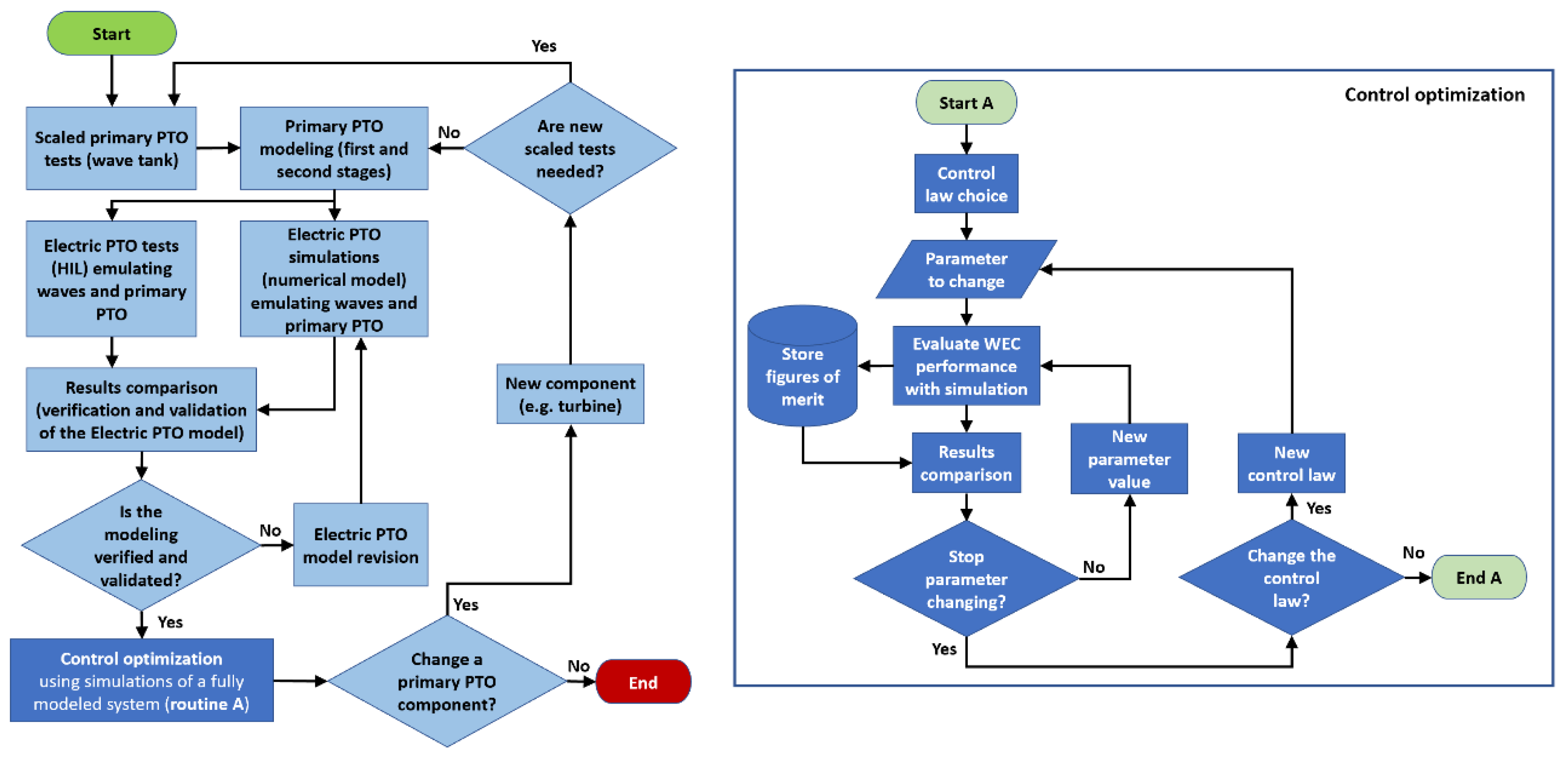
Figure 1 shows the flowchart of the proposed procedure. As it is independent of the PTO, it can be applied to different kind of WECs, both with rotating and linear electric machines. Here we will focus on systems where a rotating generator is used. Furthermore, with a scaling process the same test rig for the electric PTO tests can be used for WECs with different power rates.
It should be noted that when the primary PTO is designed for the real size, rarely it fits exactly the size of the test rig available. Then, within the allowed range of test equipment, the WEC model needs to be scaled before being used for the electric PTO tests and simulations. More details about the scaling can be found in [
18], while the scaling applied to the case study here presented will be shown in
Section 4.5.
Regarding the procedure, once the primary PTO has been chosen or defined, typically the primary PTO is tested by means of scaled prototypes in the wave flume. This allows primary PTO numerical modeling. Hence, it is possible to simulate the whole WEC focusing on the electric PTO to design it and the control. Now, can the whole model be considered valid? With large prototypes, it is possible to give an answer to this question, but generally, the cost of suitable WEC prototypes is too high to justify the necessary validation tests with real systems. The problem can be mitigated with the use of HIL testing to validate at least the electric PTO model. Then, it can be validated comparing the simulations with HIL tests results. If the model is not validated, it can be revised until the difference between tests and simulations results are not below a maximum tolerated value. Once the numerical model of the electric PTO has been validated, the optimum control law of the system can be found with an iterative final step by means of simulations. This iterative step can be carried out more easily and faster with simulations than using a HIL.
The control is optimized with nested iterative cycles where it is possible to change a parameter of the system (e.g., the turbine diameter, the moment of inertia with a flywheel, and so on), and the control law. The parameter values range and step, as well as the set of control laws, are fixed before the tests to limit the number of simulations, in turn limiting to an acceptable time-length the duration of the whole simulations set for this optimization step.
The procedure can be re-iterated for the same system if a component with different features (e.g., type of turbine) can be chosen from a set of suitable ones.
The following sections show a case study as an example of how to apply this procedure. Here are shown only some iterations to improve the efficiency of the system, just to give an example of how it is possible to tend toward an optimum solution.
The same HIL test rig has been applied to develop other WECs with high Technological Readiness Level (e.g., for the development of different WECs named REWEC3, OWC Spar-buoy, Ocean Energy buoy, and ISWEC [
19,
22]). Good results were also obtained to set a predictive control for the full-scale biradial turbine of the Mutriku OWC plant [
27].
3. HIL Test Bench
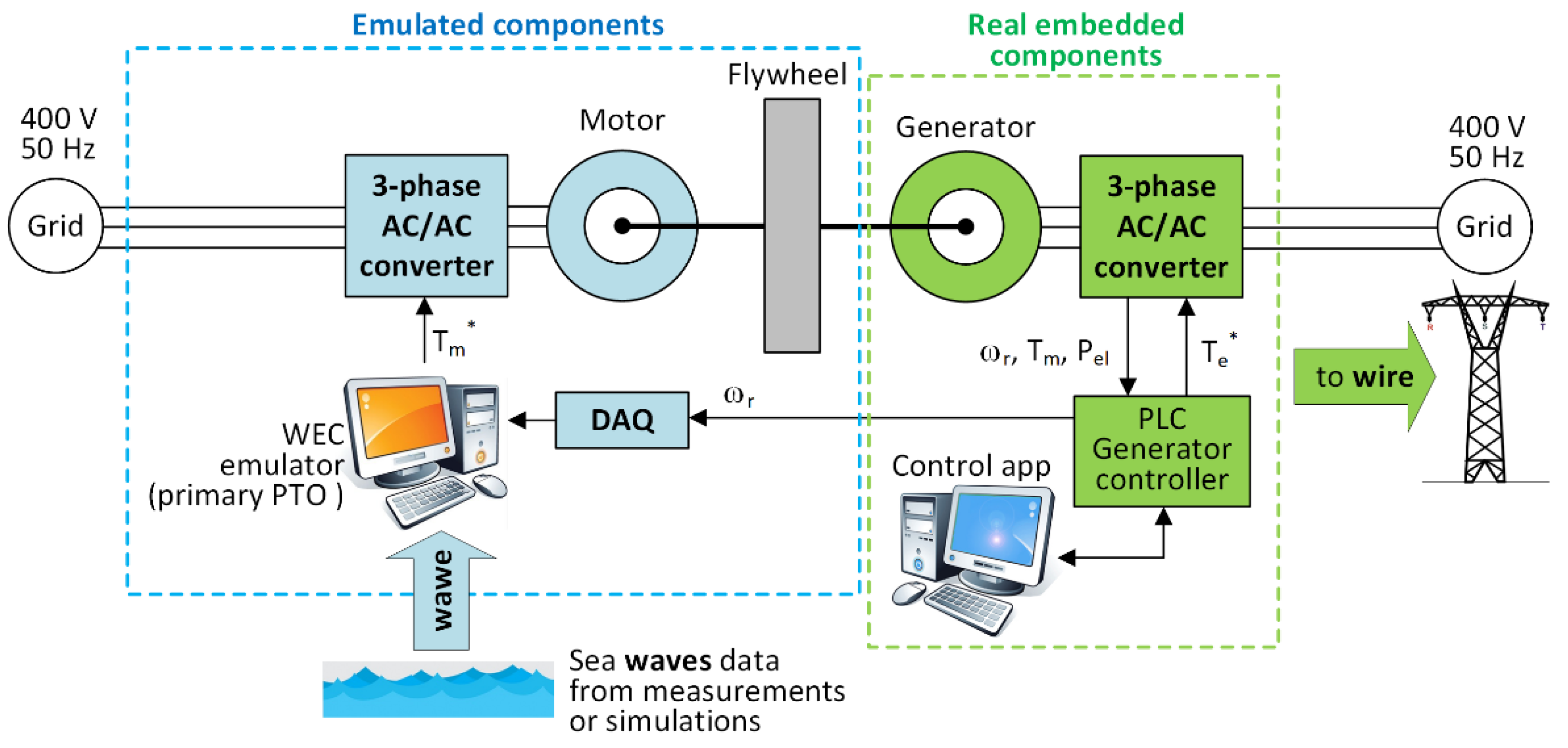
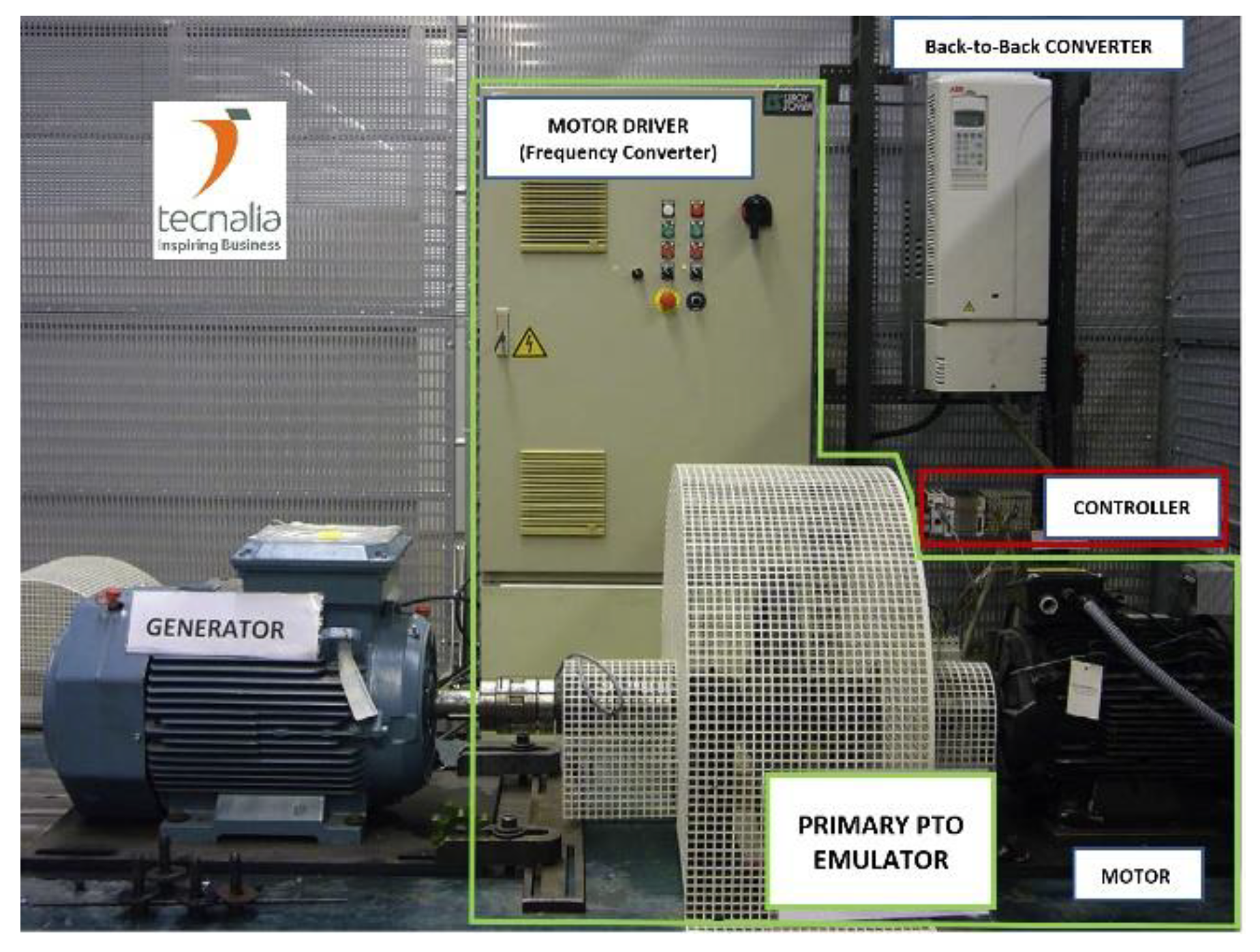
Figure 2 shows the HIL used for this work. The test bench is composed by two sections: the first one is that of the emulated parts (primary PTO in this case), the second one contains the embedded real components, in particular the generator, the AC/AC power converter and the controller.
The emulator includes the AC/AC frequency converter, the 3-phase motor, an optional flywheel, a data acquisition card (DAQ), and a PC with a dedicated software for real-time application (dSPACE with ControlDesk [
28], in this case).
The block with real components includes a generator, a power converter and a Programmable Logic Controller (PLC) that run the system control law. This section is the apparatus that connects a real WEC installed in the sea with the grid, but it can be replaced by other kind of control units based on microcontrollers and FPGAs. In the real system, the motor shaft is joined to that of the generator by a gearbox or a joint, and the system inertia can be increased up to 8 kg⋅m2 by adding a flywheel.
3.1. Wave Energy Converter Emulator
Preliminary wave flume tests, carried out scaling the device with Froude law, are frequently used to set up an interpretative model at the first stages of design, to calibrate the system hydrodynamic and the mooring. In the numerical model, the floating body hydrodynamic characteristics were found with ANSYS Aqwa, and the air flow pattern is the same described in [
26]. Please note that he turbine head losses simulated at lab scale are specific for the tests and the turbine modeling needs to be completely different at larger scales, hence the model must be integrated by a specific module for the turbine. Actually, air behaves as incompressible at low scale, and hence the numerical model should model, at large scale, also the compressibility effects.
The developed hydrodynamic MATLAB-Simulink software emulates, in the time domain, the hydraulic response of the (moored) WEC behavior under realistic sea states, the pressures in the chambers and the air flow for a given turbine head loss [
26]. The behavior of the turbine (head loss) was then added to the MATLAB-Simulink model, and everything was compiled in dSPACE, which allow interfacing the real and simulated parts of the HIL. The model still needs the turbine speed, which is read by a dSPACE real-time Interface RTI1104t, which is also used to apply the output torque to the shaft.
This approach allows emulating any energy converter using a rotating generator. The WEC is then practically emulated using a Leroy–Somer squirrel-cage induction motor type LSES 160 LUR 6-pole [
29]. The specifications of the motor are the following: voltage 400 V (delta connection), maximum speed 1800 rpm, rated speed 1468 rpm @ 50 Hz, power: 15 kW. The drive can be used with motors with a maximum speed of 3000 rpm, withstanding power surges up to 28 kW.
3.2. Electric Generator
The generator is a squirrel-cage induction machine by ABB (type M3BP 180MLA 8-pole) [
30]. Its specifications are the following: rated speed 731 rpm @ 50Hz, power 11 kW, voltage 400 V (delta connection).
An ABB ACS800 back-to-back converter connects the generator to the mains, allowing the remote control of the speed and torque by sending and analog speed/torque reference signal to the converter input. A Beckhoff CXI020 PLC controller with a series of digital and analog signal boards, which are suitable for installation on a marine energy system, implements the control. The generator and the controller communicate through several analog and digital inputs/outputs channels. The inputs of the PLC are the speed of the generator (ωr), the mechanical torque (Tm) and electrical power (Pe), while its outputs are a torque or speed set-point, depending on the implemented control.
3.3. Programming the PLC
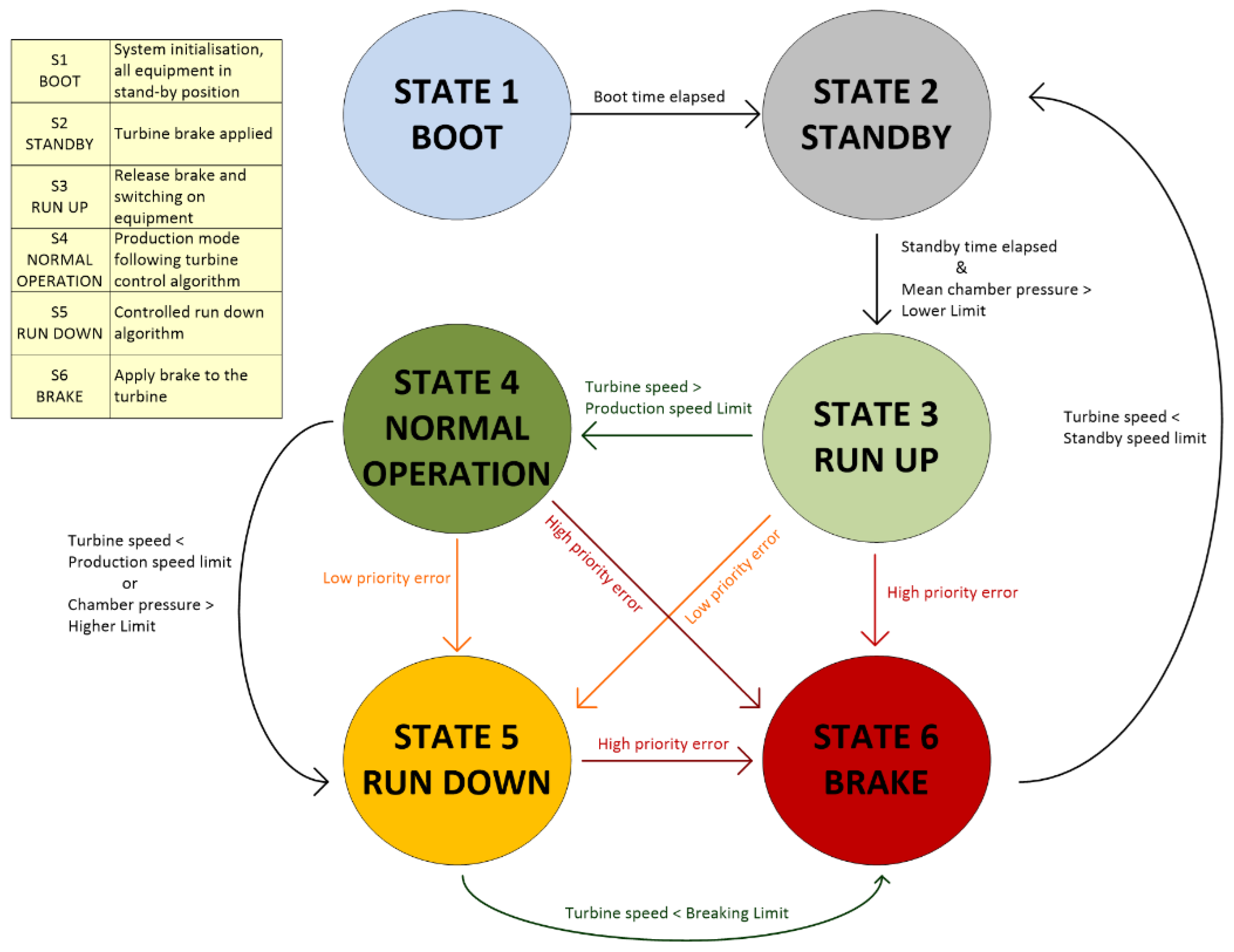
The PLC runs the control routine that handles the analog and digital inputs. It can be customized to implement various strategies for different WECs. A state machine program (
Figure 3) is implemented in the PC used for PLC programming. It goes through a series of safety check procedures and grants the operation, through a set of various control algorithms if no alarms are triggered. In this case, the output of the control routine is the electric torque (
Te*) that is applied to the generator to get the required turbine speed. This reference torque is sent to the back-to-back converter where the current control loops follow this set-point as well as control the voltage on the DC link and the injected grid power.
4. Simulink Models and Adaptations for HIL Testing Framework
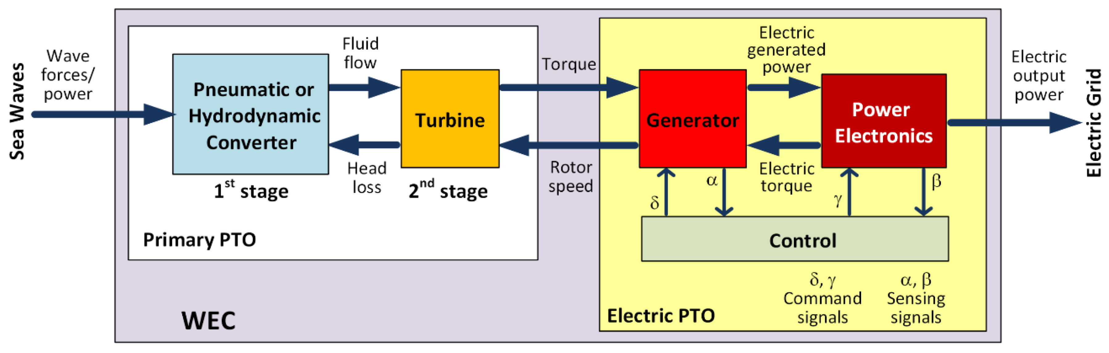
4.1. Wave-to-Wire Model
To follow the conversion path from the sea waves energy to the electrical one on the grid the W2W model [
31,
32] is commonly used (
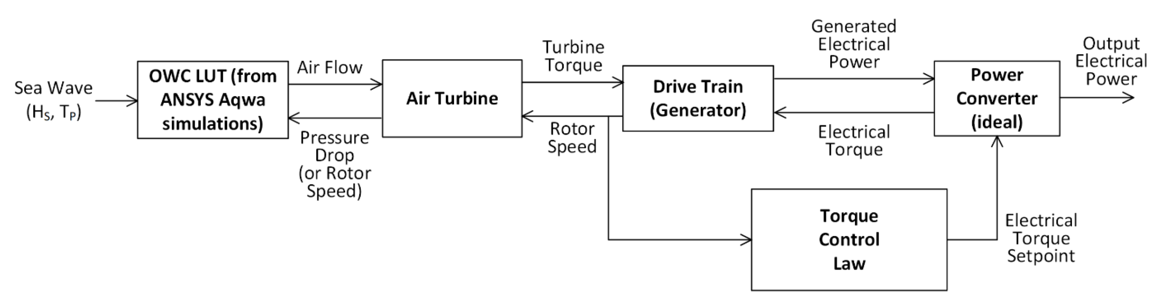
Figure 4).
Generally, the control block reads variables of the generator (e.g., rotor speed and torque) and the power electronics (e.g., output voltage and frequency) and responds with command signals to set the controlled variables to the desired values. In this case study, it will be shown how to control the rotor speed of the generator measuring the same speed and the shaft torque (evaluating with different laws the electric torque).
Once drawn the specific W2W diagram, which models the WEC at a high level of abstraction, it is possible to translate it, block by block, into a numerical model. The hydrodynamic model of the WEC is a set of MATLAB scripts and functions, where in our case the pneumatic behavior in each chamber is computed taking into account the coupling between the overall system dynamics and the turbine rigidity (in the uncoupled model, the floating body oscillations are given by the incident waves only).
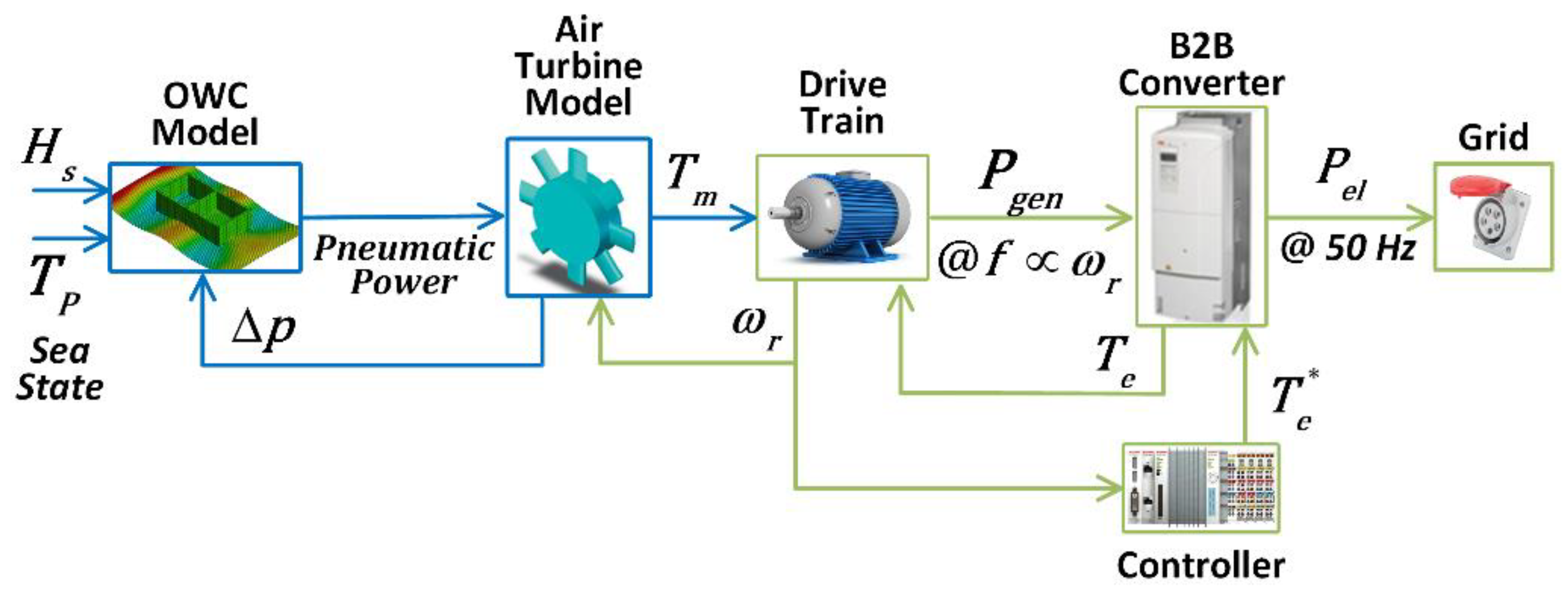
The input of the resulting W2W model shown in
Figure 5 is a regular sea state defined by the peak period
Tp, the significant wave height H
s, and the turbine head loss. Please note that to have an accurate W2W model, it is reasonable that the OWC block has a fully coupled approach, where the primary PTO pneumatic output power is influenced by the following elements in the whole conversion system.
The pressure drop across the turbine Δp is an input of the OWC model, the rotational speed ωr of the generator is an input of the air turbine model, and the load torque Te due to the electric load of the generator (B2B converter and electric grid) is an input of the drive train model. When the pneumatic power of the air flow generated by the OWC is higher than the turbine load, the turbine rotates applying a torque Tm to the generator (drive train), which produces a sinusoidal electricity at a frequency fgen proportional to the rotational speed ωr, with a generated power Pgen. The B2B converter is the interface with the electrical grid. It converts the AC input at fgen to an AC output synchronized with the voltage at 50 Hz of the grid. Pel is the power at the output of the whole WEC.
The control loop is closed to set the rotational speed at the desired value, which depends on the applied control law. Then, ωr is also the input of the controller, who generates a control signal Te*, giving information to the B2B converter on the load torque (or electrical torque) Te needed to have the desired rotational speed.
In real systems the load of the turbine is the electric PTO (generator-power converter-grid) which includes a feedback control to regulate the turbine rotational speed. Then, in practice a complete WEC is a closed-loop controlled system, which is not implemented in hydraulic lab test in small scale.
In a HIL test rig, the primary PTO must be emulated by a numerical simulator that provides the dynamic response in the time domain. These types of models usually provide the dynamic response of the WEC for a constant load on the generator. Obviously, in reality, the floating body oscillations, with its non-linear mooring, and the pressure in the chambers, depend on the real turbine head loss, which will only be defined during the HIL tests. However, models often do not take into account the physical constraints, response times and delays, and the characteristics of real equipment under normal and extreme sea-operating conditions [
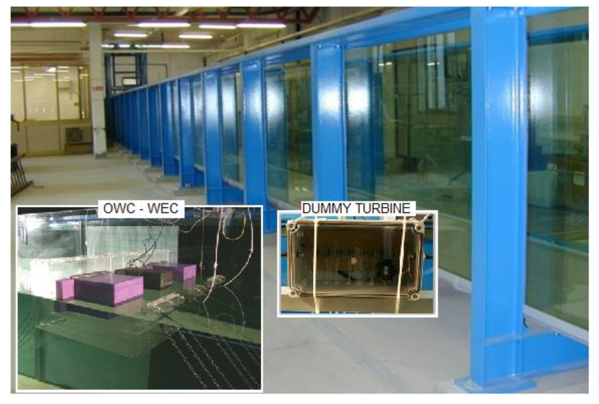
22]. One must ask whether this approximation is acceptable. Here, the problem was solved with the validation of a numerical model through wave flume tests with a dummy turbine [
25,
26]. The numerical model is calibrated to find the expected air flux induced by the incident waves, taking into account the hydrodynamic effects, for a few tested turbine head losses. Then, the numerical model is adapted to run based on a real-time input, the rotational speed. In the case taken as an example, we implemented this function with a Look-Up Table (LUT) to ensure that the air flow is obtained in real time. This made it possible to carry out closed-loop HIL tests considering the effects of time dependent turbine load on the primary PTO.
Except for the first stage of the primary PTO (OWC model), all the other parts of the systems were modeled with Simulink using LUTs and mathematical equations in order to evaluate the same variables which can be measured by the HIL bench.
Hereafter, the Simulink models will be depicted with formulae and gains applied by math and gain blocks, respectively. More information on Simulink’s symbolic notations can be found in [
33].
4.2. Air Turbines Modeling
The turbine modeling is an important step to obtain a valid model of the whole OWC. Here, to model the turbine in Simulink avoiding expensive experimental and complex 3D Computational Fluid Dynamics (CFD) simulations, a literature review was fundamental in finding equations and formulae to obtain the power and torque characteristics of different kind of turbines [
34,
35,
36].
Considering the following nomenclature:
l blade length;
n number of blades;
b chord length;
r turbine rotor radius;
A area of turbine duct;
ρ air density;
Vx air speed at the turbine inlet;
ωr rotational speed;
characteristic constant;
flow coefficient; Δ
p pressure drop across the turbine;
Q flow rate;
Tm mechanical torque;
Te electrical torque;
J moment of inertia;
Prot mechanical power at the shaft;
Ppneu pneumatic power at the inlet;
Ca input coefficient;
Ct torque coefficient;
η efficiency, the equations for the turbine are given by [
37]:
Then, the turbine efficiency can be evaluated as follows:
Table 1 resumes the parameters set for the Simulink model of different turbines: Wells, Dennis-Auld, and Impulse.
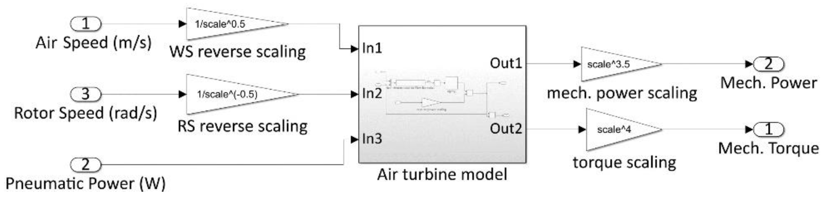
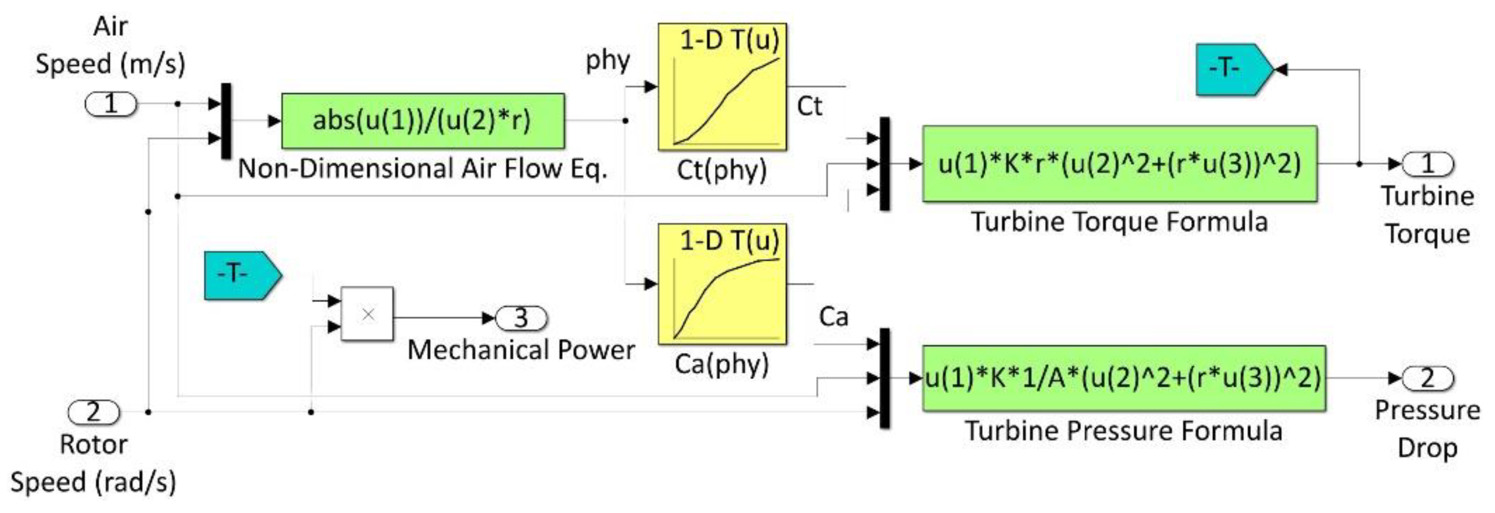
The Simulink model of the turbine is shown in
Figure 6. Considering the scaling applied (see
Section 4.5) to match the model with the HIL, it is necessary the reverse scaling of inputs and the scaling of outputs to match the air turbine model with other blocks of the whole model. The scaling is simply made by means of proportional gain blocks (triangular).
Figure 7 shows the model used for Dennis-Auld and Wells turbines. Input coefficient, efficiency, and torque coefficient from literature data were used.
Ct and
Ca are evaluated by mean of LUTs.
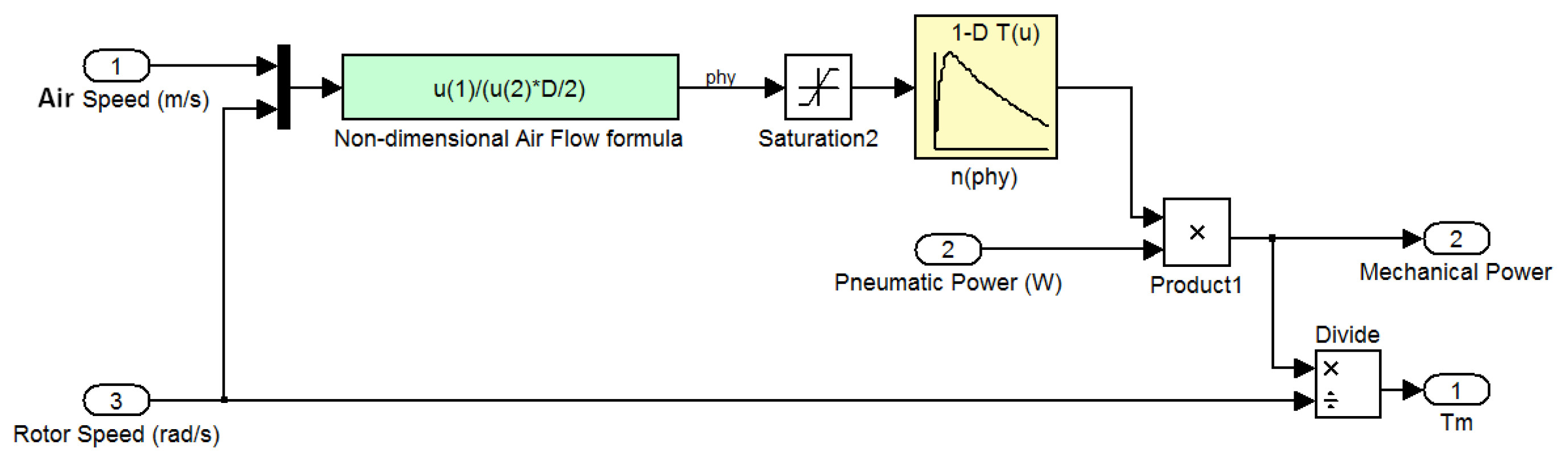
To model the Impulse turbine (
Figure 8) it was used the efficiency vs. the flow coefficient characteristic. The saturation block limits the input values given by the “Non-dimensional Air Flow Formula” used to compute the flow coefficient
φ (here u(1) is the air speed, u(2) is the rotor speed, and D is the turbine rotor diameter). This limitation is needed to match the input range of the following LUT of the turbine efficiency vs.
φ.
4.3. Drive Train Modeling
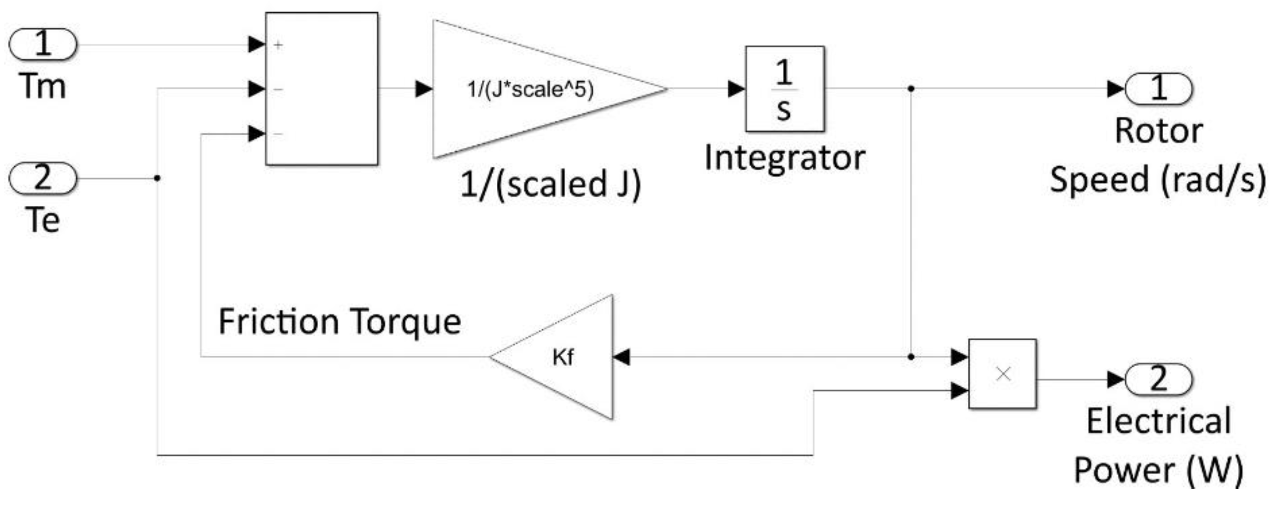
The following well-known equation of rotating mechanical systems considering the viscous friction can be used to model the generator:
where
Tfriction is the resistive frictional torque.
Figure 9 shows the Simulink model of the drive train, scaled to match the nominal torque of the WEC emulator in the HIL. It calculates the rotor speed inverting Equation (6) and the electrical power multiplying the rotor speed by the electrical torque.
4.4. Control Laws
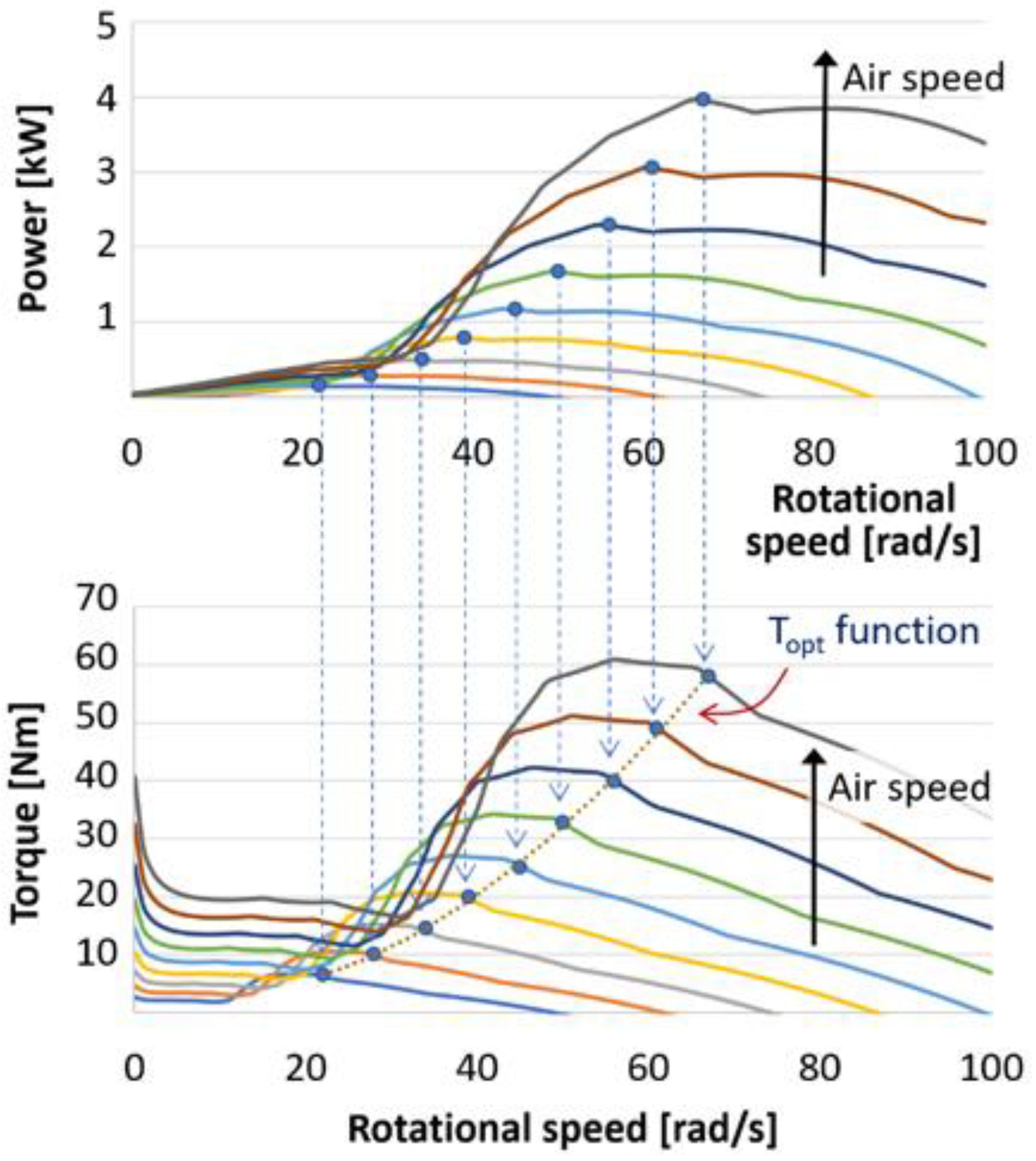
Two possible control strategies were implemented to set the torque applied to the electric generator: (i) Maximum Power Point Tracking (MPPT) which can be done using the
Topt function shown in
Figure 10; (ii) a torque control where the current rotor speed is compared to a reference value to maintain constant the speed. Typically, the former is an instantaneous control that can be effectively applied to systems with low inertia. The latter is a sea-state control that needs an offline calculation of the optimum reference speed for each sea state and is more suitable for high inertia systems. In our system, the inertia has an intermediate value, and then we cannot say in advance what is better [
38]. Thus, we chose to test both to find the optimum (the one that gives the highest power at the output given the same input). Issues related to peak-to-average power ratio and the need for overrating the power converters are not considered in this work but are well discussed in Refs. [
20,
39].
4.5. Scaling, Compensations, and Adaptations
One of the key problems of this kind of tests is that the WEC considered does not match the laboratory equipment (inertia, rated generator speed and torque, inverter nominal power). For this reason, the Simulink model has to be adapted to account for the differences with the test bench, in order to get a consistent relationship between the HIL and the models of the 2-chambers OWC considered here.
The scaling of the model should be done in order not to modify the proportionality of the forces with those of the real prototype (inertial, gravitational, viscous, elastic, and pressure). This is not feasible when the scale factor is not unitary, but in all other cases the dominant forces in the system can be found and relationship maintained.
The wave behavior is dependent by the gravity; for this reason, the Froude’s law is used, to keep the strong relationship between gravitational and inertial forces in the scaled model. Froude scaling is typical for WECs scaling (e.g., [
40,
41,
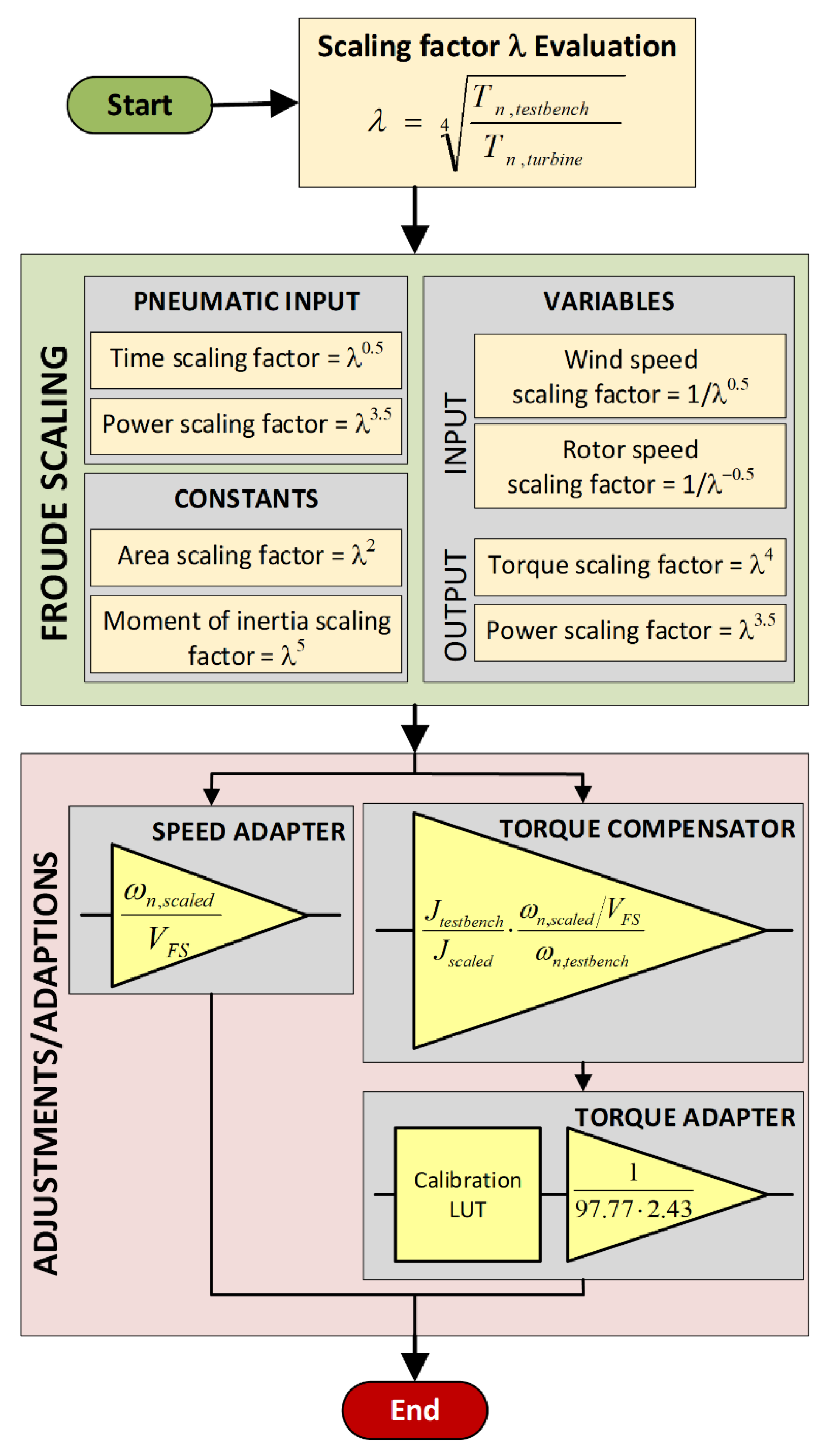
42]). The used scaling, compensations, adaptions, and the customization for this case are shown in
Figure 11. The scaling factor
λ is set to adjust the nominal torque of the turbine model
Tn,turbine to the one of the test bench
Tn,testbench. Consequently, it can be calculated by the relation:
To use the pneumatic power scaled to the HIL range, variables and constants are modified by applying Froude’s law at the output of the original blocks, while at the input the same must obviously be scaled using the inverse formulae.
Other adjustments are needed to match the values of some variables, such as the rotational speed (
ωn in
Figure 11) or the torque reference, with the electric signal that represents them at the dSPACE and the PLC interfaces.
VFS in
Figure 11 is the full-scale range of the rotational speed signal.
The same consideration was made for the simulated torque signal. Torque compensation was applied, due to the different inertia and different nominal rotational speed of the test rig and the ones of the converter under test.
4.6. Simulink Models of the Electric PTO
Following the procedure described in
Section 3 and drawing the block diagram of
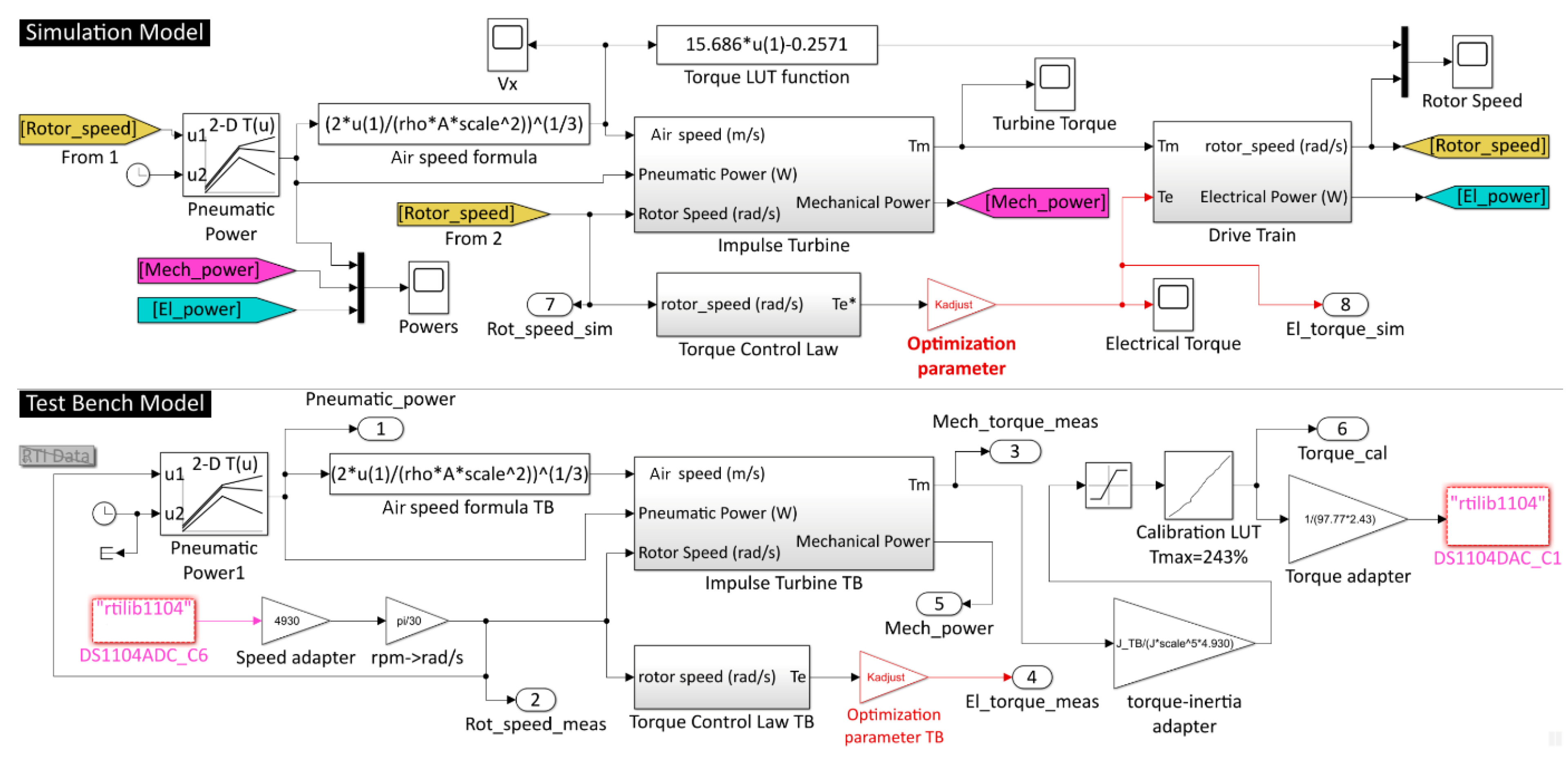
Figure 12, we obtained the Simulink model of the electric PTO of the wave converter considered here, as depicted in
Figure 13. The pneumatic power is given by a 2D LUT; the Torque Control Law block supplies the electric torque reference for the generator from the rotational speed of the turbine; the drive train block models the electric generator, while the turbine model (Impulse in
Figure 13) block models the chosen turbine giving the mechanical torque applied by the turbine to the shaft from the air speed and the rotational speed.
The power converter is assumed ideal. This is acceptable because its efficiency is high and will only depend on the power rate, and the small delay of around 1.5 cycles of the switching frequency [
43], is negligible compared to the slow dynamics of the system. Thus, it is represented by the control loops implemented on it.
As can be seen, the whole model consists of two subsystems, one to fully simulate the electric PTO (top), and one for the HIL where the drive train is real (bottom) and the rotor speed can be measured. Then, in the Test Bench Model there is not the drive train block, but there are two blocks of the hardware dSPACE real-time Interface RTI1104t to set the torque and to read the rotor speed. The speed coming from the interface is adapted according to the scheme of
Figure 11 and converted in rad/s, while the torque computed by the Impulse Turbine TB block needs to be calibrated and adapted, still using the scheme of
Figure 11. In the Test Bench Model, the Torque Control Law TB to evaluate
Te* is not strictly necessary, because this signal is really generated by the PLC. We put this block only to easily export the signal data in MATLAB.
The gain block with the optimization parameter comes from a verification step that required a revision of the model according to the procedure of
Figure 1, as will be shown in the following section.
In addition to MPPT implemented by the Torque Control Law block in
Figure 13 applying the optimum torque function of
Figure 10, we considered other two kinds of control laws to set a constant speed: an on-off strategy (
Figure 14), and a Proportional–Integral (PI) regulator (
Figure 15).
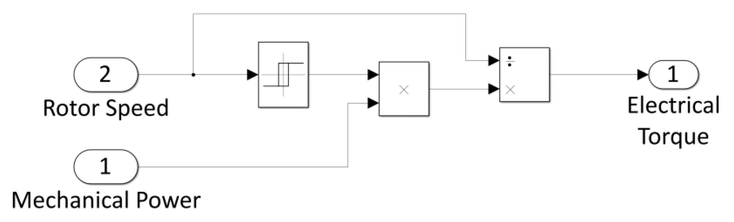
For the on-off control, a Simulink Relay block is used to switch between an electrical torque evaluated dividing the mechanical power by the rotor speed and a null torque. The hysteresis coming from different thresholds for the switch on and the switch off is also used to filter the noise added to the rotor speed signal.
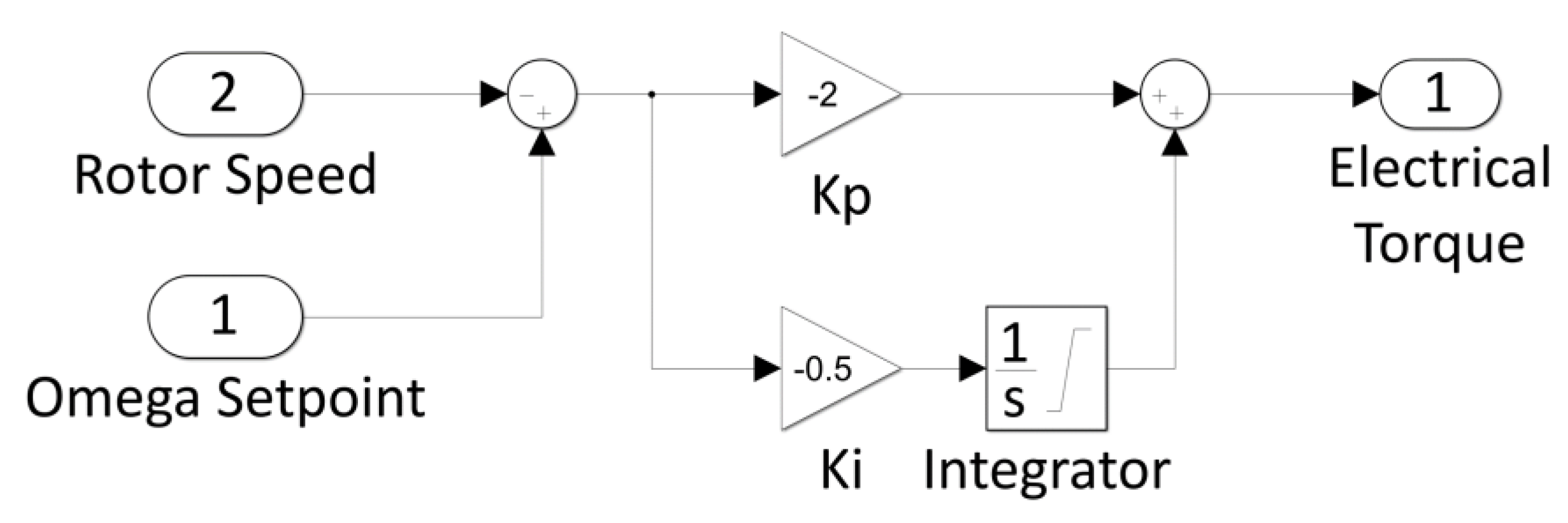
The PI regulator in
Figure 15 is set to implement the function:
where
ωsp is the constant set-point of the rotor speed,
ωr(
t) is the actual rotor speed,
Kp and
Ki are the proportional and the integral coefficients, respectively.
5. Experimental Results
First, a set of tests was conducted to assess which turbine is the most suitable for the OWC being studied. In this case, given the turbines in
Table 1, the best choice was the Impulse turbine, because it led to obtain the highest average powers at the shaft with all the considered sea wave conditions.
Before the second phase of the work, a test protocol to plan the experimental test following the algorithm in
Figure 1 was prepared. It is presented in
Table 2. For each case of
Table 2, the test was repeated considering the six sea states in
Table 3.
The next phases were carried out to get a clearer correlation between the simulations and the HIL experiments. Each test described was repeated for all the sea states listed in the right-hand column.
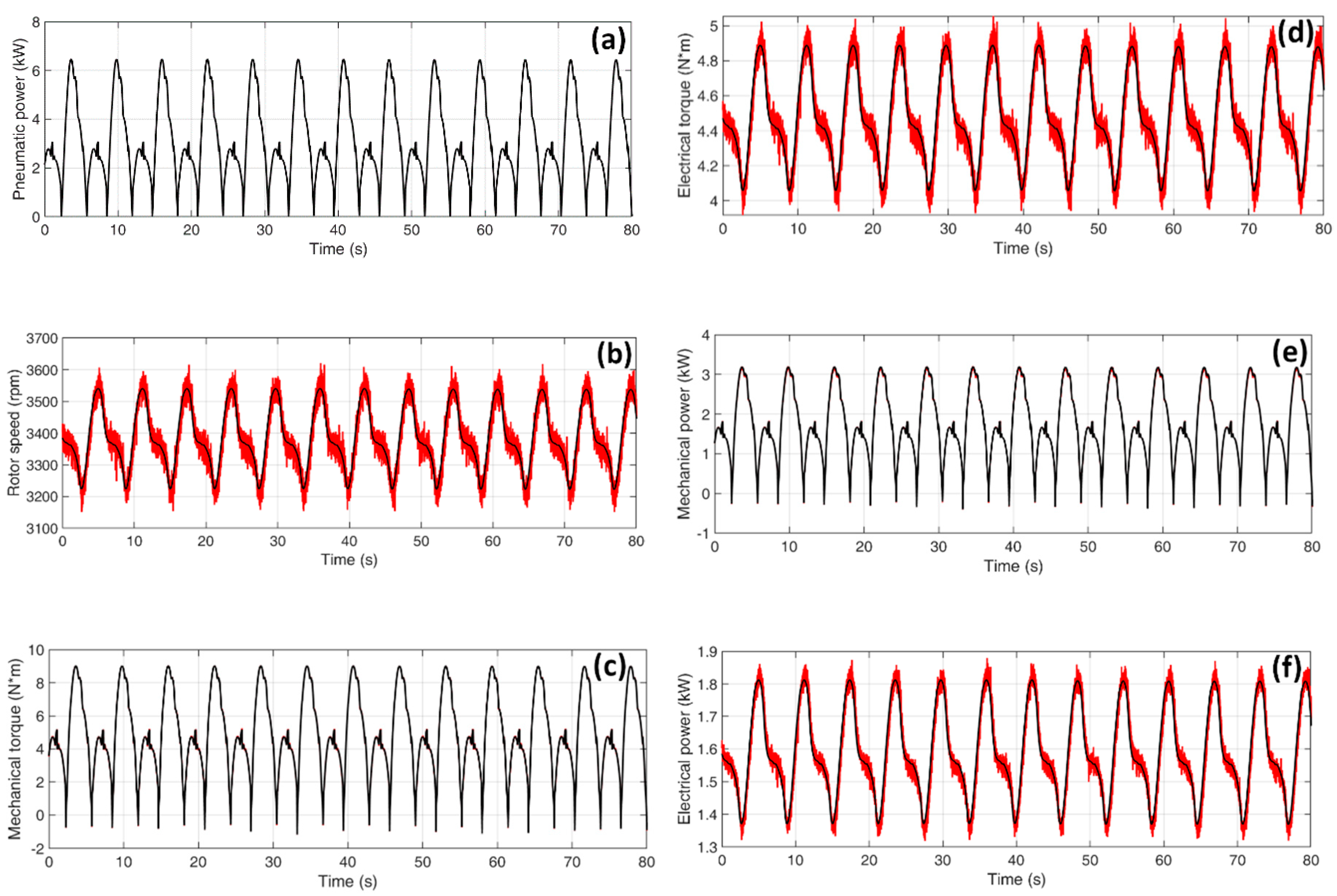
The main goal was to verify that the models are sufficiently accurate for future design and optimization purposes. For this reason, we compared simulations with measurements. For example,
Figure 16 shows measured and simulated power, torque and rotor speed for an Impulse turbine and
Hs = 1.6 m. As shown, the match between measurements and simulations is very good.
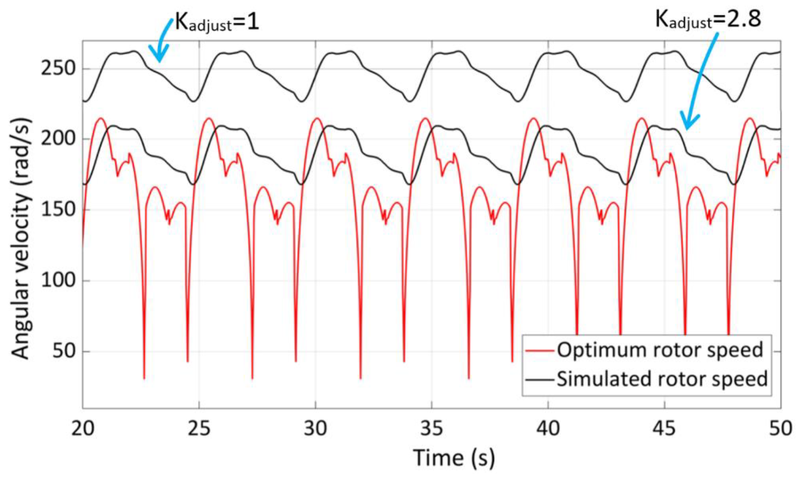
The test with the HIL showed that applying the MPPT control for the torque as obtained from the characteristics in
Figure 10 for an Impulse turbine (setting
Kadjust = 1 in the model of
Figure 13), the rotational speed is always higher than the optimum one (e.g., as shown in
Figure 16 with
Hs = 1 m). The rotor speed cannot vary rapidly as the optimum one due to the inertia (in this case, at the real scale, it is 0.1 kg⋅m
2).
Thus, to increase the power at the generator output (drive train) the rotational speed can be lowered to be closer to the optimum, applying to the drive train a higher electrical torques, by setting Kadjust > 1.
To better analyze what happens changing Kadjust, the mean power measured during the tests can be taken as reference.
Let <P
pneu> be the mean pneumatic power at the turbine inlet, <P
mech> the mean power at the shaft of the turbine and <P
el> the mean power at the output of the electric generator, then these powers change with K
adjust. For each sea state, an optimum value of K
adjust can be found to obtain the maximum efficiency of the whole converter. For example, considering the conditions of
Figure 16, the <P
el> can be increased from 3.2 kW to 4 kW changing K
adjust from 1 to 2.8 as shown in
Figure 17. This value results the one that gives the highest mean generator power when H
s = 1 m, then optimizing the applied control law only for a specific sea-state.
The constant speed control with on-off law has been demonstrated to be the less efficient, while the MPPT is the best.
Table 4 and
Table 5 show the results obtained with the MPPT control and the constant speed control with PI regulator, respectively. Using the constant speed control with a PI regulator, the total efficiency is lower, around 10% less, than the one obtained with the MPPT for all the sea states. In addition, the MPPT is an adaptive control type and is to be preferred because on the opposite of the fixed speed control, it is not sea-state dependent.
With the MPPT control, Kadjust can be changed to maximize the <Pel>. At each wave height, the optimum Kadjust is different. Then, the control law is dependent on the incident wave.
6. Conclusions
In this paper, a method to perform experiments coupled to numerical analysis on the electrical PTO of a WEC at the early stages of development has been thoroughly investigated.
The relevance of this paper mainly stays on the proposed methodology, which links wave flume (
Figure 18) and HIL (
Figure 19) tests carried out at different scales: hydraulic models based on physical model tests in the wave flume (e.g., in scale 1:20) should not be built around a closed dummy turbine model, but should be interpreted by a model that can be coupled to a HIL test rig (e.g., in scale 1:5).
The proposed procedure, schematically presented in
Figure 1, has been described also with an example, considering some iterations to improve the power at the output of the generator. The aim was to significantly increase efficiency at an early design stage through the choice of the turbine and the control regulation. To do this, we needed to solve several aspects of coupled modeling, and the procedure described in this paper is our best solution for this combined hydrodynamic-electrical approach.
The experiments allow one to verify the validity of the modeling technique applied with the pneumatic power generated by 3D hydro-pneumatic simulations, and to demonstrate that the method can be useful to design the power conversion equipment also thanks to accurate development of the WEC’s control strategies. Although the method is in principle extendible to irregular wave conditions, the actual applicability under irregular sea states has not yet to be proved.
About the OWC considered here, the following main results were obtained.
The pneumatic power (as the electrical and mechanical ones) significantly depends on the turbine working conditions (a fully coupled modeling approach is important for this type of device).
The MPPT control is more effective in following the optimum rotational speed than a torque control where the actual rotor speed is kept as much as possible equal to a set-point.
The control law depends on the incident wave. Then, we can say that to improve the efficiency of the system, the OWC should be equipped with a system that measures the incident wave.
The work here presented may be extended and applied to a more advanced design (e.g., considering a predictive strategy with artificial neural network) of the control system for the OWC taken as reference, to improve its performance. The usefulness of the HIL test rig is in fact demonstrated not only by the study case of this work, but also by the works in [
19] and [
22] for different WECs at the design stage. More recently, it has been validated also for a real [
27], but it was never defined and structured as in the present work.
Author Contributions
Conceptualization, methodology, software, modeling, validation, and formal analysis, N.D., E.R., J.L., F.G., P.C., P.R. and L.M.; Investigation, N.D., P.C., F.G., L.M. and F.X.F.; Resources, and data analysis, N.D., L.M. and F.G.; Writing-Review & Editing, N.D., E.R., F.X.F., F.G., P.C. and L.M. All authors have read and agreed to the published version of the manuscript.
Funding
This work was supported by MARINET, a European Community—Research Infrastructure Action under the FP7 “Capacities” Specific Programme, grant agreement n. 262552.
Acknowledgments
The authors would like to express special thanks to the editors and anonymous reviewers for their constructive comments on this manuscript.
Conflicts of Interest
The authors declare no conflict of interest.
References
- MaRINET Research Reports. Available online: http://www.marinet2.eu/archive-reports-2/research-reports/ (accessed on 6 January 2020).
- Ocean Energy Strategic Roadmap 2016, Building Ocean Energy for Europe. Available online: https://webgate.ec.europa.eu/maritimeforum/sites/maritimeforum/files/OceanEnergyForum_Roadmap_Online_Version_08Nov2016.pdf (accessed on 6 January 2020).
- IEA-Ocean Energy Systems. Annex II-Implementing Agreement on Ocean Energy Systems-Report 2003; Nielsen, K., Ed.; IEA-Ocean Energy Systems: Lisbon, Portugal, 2003. [Google Scholar]
- Davies, P. Guidelines for the Design Basis of Marine Energy Converters ANNEX II-Task 3.3 Guidelines on Design, Safety and Installation Procedures; European Marine Energy Centre BSI: London, UK, 2009. [Google Scholar]
- Nielsen, K. ANNEX II Extension-Development of Recommended Practices for Testing and Evaluating Ocean Energy Systems-Summary Report August 2010; Ramboll: København, Denmark, 2010. [Google Scholar]
- Committee of Ocean Energy Systems. Annual Report-An Overview of Ocean Energy Activities in 2017; Brito e Melo, A., Jeffrey, H., Eds.; Executive Committee of Ocean Energy Systems: Lisbon, Portugal, 2017. [Google Scholar]
- Executive Committee of Ocean Energy Systems. An Overview of Ocean Energy Activities in 2018; Brito e Melo, A., Jeffrey, H., Eds.; Executive Committee of Ocean Energy Systems: Lisbon, Portugal, 2019. [Google Scholar]
- Shalby, M.; Dorrell, D.G.; Walker, P. Multi–chamber oscillating water column wave energy converters and air turbines: A review. Int. J. Energy Res. 2018, 43, 681–696. [Google Scholar] [CrossRef]
- Delmonte, N.; Barater, D.; Giuliani, F.; Cova, P.; Buticchi, G. Oscillating water column power conversion: A technology review. In Proceedings of the IEEE Energy Conversion Congress and Exposition (ECCE), Pittsburgh, PA, USA, 14–18 September 2014; pp. 1852–1859. [Google Scholar]
- Delmonte, N.; Barater, D.; Giuliani, F.; Cova, P.; Buticchi, G. Review of oscillating water column converters. IEEE Trans. Ind. Appl. 2016, 52, 1698–1710. [Google Scholar] [CrossRef]
- Falcão, A.F.O.; Henriques, J.C.C. Oscillating-water-column wave energy converters and air turbines: A review. Renew. Energy 2016, 85, 1391–1424. [Google Scholar] [CrossRef]
- Carnegie Clean Energy. Available online: https://www.carnegiece.com (accessed on 31 December 2019).
- Seabased. Available online: https://www.seabased.com (accessed on 31 December 2019).
- Wello–Penguin. Available online: https://wello.eu/technology (accessed on 31 December 2019).
- Boake, C.B.; Whittaker, T.J.T.; Folley, M.; Ellen, H. Overview and Initial Operational Experience of the LIMPET Wave Energy Plant. In Proceedings of the 12th International Offshore and Polar Engineering Conference, Kitakyushu, Japan, 26–31 May 2002; pp. 586–594. [Google Scholar]
- Falcão, A.D.O. The shoreline OWC wave power plant at the Azores. In Proceedings of the 4th European Wave Energy Conference, Aalborg, Denmark, 4–6 December 2000; pp. 42–48. [Google Scholar]
- Faÿ, F.; Robles, E.; Marcos, M.; Aldaiturriaga, E.; Camacho, E.F. Sea trial results of a predictive algorithm at the Mutriku Wave power plant and controllers assessment based on a detailed plant model. Renew. Energy 2020, 146, 1725–1745. [Google Scholar] [CrossRef]
- Report on Dynamic Test Procedures. MARINET-document n. D4.02: 2014. Available online: http://www.marinet2.eu/wp-content/uploads/2017/04/D4.2-Report-on-dynamic-test-procedures-1.pdf (accessed on 9 April 2020).
- Armstrong, S.; Rea, J.; Faÿ, F.; Robles, E. Lessons learned using electrical research test infrastructures to address the electrical challenges faced by ocean energy developers. Int. J. Mar. Energy 2015, 12, 46–62. [Google Scholar] [CrossRef]
- Tedeschi, E.; Molinas, M. Tunable Control Strategy for Wave Energy Converters With Limited Power Takeoff Rating. IEEE Trans. Ind. Electron. 2012, 59, 3838–3846. [Google Scholar] [CrossRef]
- Trapanese, M.; Boscaino, V.; Cipriani, G.; Curto, D.; Dio, V.D.; Franzitta, V. A Permanent Magnet Linear Generator for the Enhancement of the Reliability of a Wave Energy Conversion System. IEEE Trans. Ind. Electron. 2019, 66, 4934–4944. [Google Scholar] [CrossRef]
- Bracco, G.; Giorcelli, E.; Mattiazzo, G.; Orlando, V.; Raffero, M. Mechatronics Hardware-In-the-Loop test rig for the ISWEC wave energy system. Mechatronics 2015, 25, 11–17. [Google Scholar] [CrossRef]
- De Koker, K.L.; Crevecoeur, G.; Vantorre, M.; Vandevelde, L. Design of a Froude Scaled PTO Lab Setup. In Proceedings of the 11th European Wave and Tidal Energy Conference, Nantes, France, 6–11 September 2015. [Google Scholar]
- Henriques, J.C.C.; Gato, L.M.C.; Falcão, A.F.O.; Robles, E.; Faÿ, F.X. Latching control of a floating oscillating-water-column wave energy converter. Renew. Energy 2016, 90, 229–241. [Google Scholar] [CrossRef]
- Martinelli, L.; Ruol, P.; Fassina, E.; Giuliani, F.; Delmonte, N. A wave-2-wire experimental investigation of the new ‘Seabreath’ wave energy converter: The hydraulic response. In Proceedings of the 34th Conference on Coastal Engineering, Seoul, Korea, 15–20 June 2014. [Google Scholar]
- Martinelli, L.; Pezzutto, P.; Ruol, P. Experimentally based model to size the geometry of a new OWC device, with reference to the mediterranean sea wave environment. Energies 2013, 6, 4696–4720. [Google Scholar] [CrossRef]
- Faÿ, F.X.; Henriques, J.C.; Kelly, J.; Mueller, M.; Aobusara, M.; Sheng, W.; Marcos, M. Comparative assessment of control strategies for the biradial turbine in the Mutriku OWC plant. Renew. Energy 2020, 146, 2766–2784. [Google Scholar] [CrossRef]
- dSPACE Release 7.4. Available online: https://www.dspace.com/en/pub/home/products/releases/relarchive/dspace_release_74.cfm#143_12926 (accessed on 25 April 2020).
- IMfinity® 3-phase Induction Motors. Leroy-Somer catalogue 5147 en-2016.09/f. Available online: http://mlatsos.gr/img/cms/LS-Catalogue-5147f_en.pdf (accessed on 9 April 2020).
- Low Voltage-Process Performance Motors. ABB Motors and Generators Catalogue 9AKK105944 EN 02-2020. Available online: https://library.e.abb.com/public/0653647a8fe94c888731ff6fa3fee417/Process%20perf%209AKK105944%20EN%2002-2020%20Final.pdf (accessed on 9 April 2020).
- Penalba, M.; Ringwood, J.V. A high-fidelity wave-to-wire model for wave energy converters. Renew. Energy 2019, 134, 367–378. [Google Scholar] [CrossRef]
- Tedeschi, E.; Santos-Mugica, M. Modeling and Control of a Wave Energy Farm Including Energy Storage for Power Quality Enhancement: The Bimep Case Study. IEEE Trans. Power Syst. 2014, 29, 1489–1497. [Google Scholar] [CrossRef]
- Get Started with Simulink. Available online: https://it.mathworks.com/help/simulink/getting-started-with-simulink.html (accessed on 30 April 2020).
- Gareev, A. Analysis of Variable Pitch air Turbines for Oscillating Water Column (OWC) Wave Energy Converters. Ph.D. Thesis, University of Wollongong, School of Mechanical, Materials and Mechatronic Engineering, Wollongong, Australia, 2011. [Google Scholar]
- Falcão, A.F.O.; Gato, L.M.C. Air turbines. In Comprehensive Renewable Energy; Sayigh, A., Bahaj, A.S., Eds.; Elsevier: Amsterdam, The Netherlands, 2012; pp. 111–149. [Google Scholar]
- Setoguchi, K.K.T.; Raghunathan, S.; Takao, M. Air-Turbine with Self-Pitch-Controlled Blades for Wave Energy Conversion (Estimation of Performances in Periodically Oscillating Flow). Int. J. Rotating Mach. 1997, 3, 233–238. [Google Scholar] [CrossRef]
- Setoguchi, T.; Santhakumar, S.; Maeda, H.; Takao, M.; Kaneko, K. A review of impulse turbines for wave energy conversion. Renew. Energy 2001, 23, 261–292. [Google Scholar]
- Ceballos, S.; Rea, J.; Lopez, I.; Pou, J.; Robles, E.; O’Sullivan, D.L. Efficiency optimization in low inertia wells turbine-oscillating water column devices. IEEE Trans. Energy Convers. 2013, 28, 553–564. [Google Scholar] [CrossRef]
- Tedeschi, E.; Carraro, M.; Molinas, M.; Mattavelli, P. Effect of Control Strategies and Power Take-Off Efficiency on the Power Capture From Sea Waves. IEEE Trans. Energy Convers. 2011, 26, 1088–1098. [Google Scholar] [CrossRef]
- Palm, J.; Eskilsson, C.; Bergdahl, L.; Bensow, R.E. Assessment of Scale Effects, Viscous Forces and Induced Drag on a Point-Absorbing Wave Energy Converter by CFD Simulations. J. Mar. Sci. Eng. 2018, 6, 124. [Google Scholar] [CrossRef] [Green Version]
- Schmitt, P.; Elsäßer, B. The application of Froude scaling to model tests of Oscillating Wave Surge Converters. Ocean Eng. 2017, 141, 108–115. [Google Scholar] [CrossRef] [Green Version]
- Bosma, B.; Lewis, T.; Brekken, T.; Von Jouanne, A. Wave Tank Testing and Model Validation of an Autonomous Wave Energy Converter. Energies 2015, 8, 8857–8872. [Google Scholar] [CrossRef]
- Wang, X.; Harnefors, L.; Blaabjerg, F. Unified Impedance Model of Grid-Connected Voltage-Source Converters. IEEE Trans. Power Electron. 2018, 33, 1775–1787. [Google Scholar] [CrossRef] [Green Version]
Figure 1.
Flowchart of the procedure to set and optimize the control of a WEC at the early development stages.
Figure 1.
Flowchart of the procedure to set and optimize the control of a WEC at the early development stages.
Figure 2.
Schematic architecture of the test rig setup.
Figure 2.
Schematic architecture of the test rig setup.
Figure 3.
Diagram of the state machine executed by the PLC.
Figure 3.
Diagram of the state machine executed by the PLC.
Figure 4.
Wave-to-wire model of a wave energy converter.
Figure 4.
Wave-to-wire model of a wave energy converter.
Figure 5.
HIL block diagram: the OWC is fully coupled with the turbo-generator.
Figure 5.
HIL block diagram: the OWC is fully coupled with the turbo-generator.
Figure 6.
Simulink model with rotor and wind speeds as inputs, and power and torque at the shaft as outputs.
Figure 6.
Simulink model with rotor and wind speeds as inputs, and power and torque at the shaft as outputs.
Figure 7.
Simulink model of air turbine using the torque and the input coefficients.
Figure 7.
Simulink model of air turbine using the torque and the input coefficients.
Figure 8.
Simulink model of air turbine using efficiency vs. flow coefficient characteristic.
Figure 8.
Simulink model of air turbine using efficiency vs. flow coefficient characteristic.
Figure 9.
Simulink model of the drive train.
Figure 9.
Simulink model of the drive train.
Figure 10.
Power characteristic of the Impulse turbine in
Table 1. The air speed varies from 4 m/s to 12 m/s with a step of 1 m/s.
Figure 10.
Power characteristic of the Impulse turbine in
Table 1. The air speed varies from 4 m/s to 12 m/s with a step of 1 m/s.
Figure 11.
Scheme of the methodology for scaling, compensations, and adaptations that must be applied to the original model for the two-chambers OWC here considered.
Figure 11.
Scheme of the methodology for scaling, compensations, and adaptations that must be applied to the original model for the two-chambers OWC here considered.
Figure 12.
PTO block diagram for Simulink modeling.
Figure 12.
PTO block diagram for Simulink modeling.
Figure 13.
Simulink model of the electric PTO with an MPPT control law.
Figure 13.
Simulink model of the electric PTO with an MPPT control law.
Figure 14.
Detail of the on-off constant rotational speed control law.
Figure 14.
Detail of the on-off constant rotational speed control law.
Figure 15.
Detail of the PI regulator.
Figure 15.
Detail of the PI regulator.
Figure 16.
Simulated (black traces) and measured (red traces) variables: (a) pneumatic power; (b) rotor speed; (c) mechanical torque; (d) electrical torque; (e) mechanical power; (f) electrical power. Sea state: Hs = 1.6 m, Ts = 5.1 s. Turbine: Impulse. Control law: MPPT.
Figure 16.
Simulated (black traces) and measured (red traces) variables: (a) pneumatic power; (b) rotor speed; (c) mechanical torque; (d) electrical torque; (e) mechanical power; (f) electrical power. Sea state: Hs = 1.6 m, Ts = 5.1 s. Turbine: Impulse. Control law: MPPT.
Figure 17.
Optimum and simulated rotor speeds with
Hs = 1 m,
Tp = 4.3 s using the model of
Figure 13.
Figure 17.
Optimum and simulated rotor speeds with
Hs = 1 m,
Tp = 4.3 s using the model of
Figure 13.
Figure 18.
Wave flume of the Maritime Laboratory at the University of Padua.
Figure 18.
Wave flume of the Maritime Laboratory at the University of Padua.
Figure 19.
Test rig at the Tecnalia Electrical PTO Lab.
Figure 19.
Test rig at the Tecnalia Electrical PTO Lab.
Table 1.
Parameters of the turbines modeled for the tests.
Table 1.
Parameters of the turbines modeled for the tests.
| | Turbine |
|---|
| Parameter | Wells | Dennis-Auld | Impulse |
|---|
| r [m] | 0.25 | 0.25 | 0.25 |
| l [m] | 0.16 | 0.16 | 0.15 |
| b [m] | 0.055 | 0.1 | 0.1 |
| n | 10 | 40 | 20 |
| A [m2] | 0.196 | 0.196 | 0.196 |
| J [kg⋅m2] | 0.2 | 0.5 | 0.1 |
Table 2.
Test plan applying different control laws with the Impulse turbine.
Table 2.
Test plan applying different control laws with the Impulse turbine.
| Test ID | Description |
|---|
| #1 | MPPT control law (torque vs. rotational speed) |
| #2 | Adjustment of the control law adopted for #1 tests to get the maximum output power at the grid |
| #3 | Constant speed control with on-off law |
| #4 | Constant speed control with PI |
Table 3.
Sea states applied to each control law of the test plan in
Table 2.
Table 3.
Sea states applied to each control law of the test plan in
Table 2.
| | Sea state ID (Regular Waves) |
|---|
| #1 | #2 | #3 | #4 | #5 | #6 |
|---|
| Hs [m] | 0.6 | 0.8 | 1.0 | 1.2 | 1.4 | 1.6 |
| TP [s] | 3.1 | 3.6 | 4.0 | 4.4 | 4.7 | 5.1 |
Table 4.
Powers and efficiencies obtained considering an Impulse turbine, with MPPT control; Kadjust = 1.
Table 4.
Powers and efficiencies obtained considering an Impulse turbine, with MPPT control; Kadjust = 1.
| | Average Power [W] | Efficiency [%] |
|---|
| Hs [m] | Pneumatic | Mechanical | Electrical | Turbine | Generator | Total |
|---|
| 0.6 | 1941 | 1364 | 999 | 70.3 | 73.2 | 51.5 |
| 0.8 | 3883 | 2655 | 2065 | 68.4 | 77.8 | 53.2 |
| 1 | 5894 | 4326 | 3256 | 73.4 | 75.3 | 55.2 |
| 1.2 | 7799 | 5258 | 4295 | 67.4 | 81.7 | 55.1 |
| 1.4 | 9658 | 6503 | 5385 | 67.3 | 82.8 | 55.8 |
| 1.6 | 11,820 | 7953 | 6663 | 67.3 | 83.8 | 56.4 |
Table 5.
Powers and efficiencies obtained considering an Impulse turbine, with constant speed control (PI regulator).
Table 5.
Powers and efficiencies obtained considering an Impulse turbine, with constant speed control (PI regulator).
| | Average Power [W] | Efficiency [%] |
|---|
| Hs [m] | Pneumatic | Mechanical | Electrical | Turbine | Generator | Total |
|---|
| 0.6 | 1974 | 1526 | 824 | 77.3 | 54.0 | 41.7 |
| 0.8 | 3999 | 3075 | 1845 | 76.9 | 60.0 | 46.1 |
| 1 | 3975 | 2960 | 1774 | 74.5 | 59.9 | 44.6 |
| 1.2 | 8053 | 6135 | 3681 | 76.2 | 60.0 | 45.7 |
| 1.4 | 10,168 | 7777 | 4666 | 76.5 | 60.0 | 45.9 |
| 1.6 | 12,265 | 9229 | 5537 | 75.2 | 60.0 | 45.1 |
© 2020 by the authors. Licensee MDPI, Basel, Switzerland. This article is an open access article distributed under the terms and conditions of the Creative Commons Attribution (CC BY) license (http://creativecommons.org/licenses/by/4.0/).

 ,
, 


