Demand Response of Residential Houses Equipped with PV-Battery Systems: An Application Study Using Evolutionary Algorithms

Abstract

Households equipped with distributed energy resources, such as storage units and renewables, open the possibility of self-consumption of on-site generation, sell energy to the grid, or do both according to the context of operation. In this paper, a model for optimizing the energy resources of households by an energy service provider is developed. We consider houses equipped with technologies that support the actual reduction of energy bills and therefore perform demand response actions. A mathematical formulation is developed to obtain the optimal scheduling of household devices that minimizes energy bill and demand response curtailment actions. In addition to the scheduling model, the innovative approach in this paper includes evolutionary algorithms used to solve the problem under two optimization approaches: (a) the non-parallel approach combine the variables of all households at once; (b) the parallel-based approach takes advantage of the independence of variables between households using a multi-population mechanism and independent optimizations. Results show that the parallel-based approach can improve the performance of the tested evolutionary algorithms for larger instances of the problem. Thus, while increasing the size of the problem, namely increasing the number of households, the proposed methodology will be more advantageous. Overall, vortex search overcomes all other tested algorithms (including the well-known differential evolution and particle swarm optimization) achieving around 30% better fitness value in all the cases, demonstrating its effectiveness in solving the proposed problem.

1. Introduction

In the current environmental world scenario, countries are adopting a series of counter measures in what regards to the use of energy, renewable sources and DG (Distributed generator) [1]. In fact, the European Union, according to the EU (European Union) renewable energy directive (2009/28/EC), is pushing to their country members to achieve strict targets such as the of penetration of 20% of renewables into the energy mix by 2020, and increase the quantity up to by 100% by 2050. Thus, in order to achieve such ambitious targets, it is expected a systematic and elaborated transformation of the electrical grid, in line with the ambitions of the EU [2].

In this scenario, new technologies such as PV (Photovoltaic) panels and battery systems emerge as a viable solution to promote the penetration of renewables at the local level of the distribution networks. Households equipped with PV generation and storage units became small producers (the so-called prosumers due to their condition of consumer and producer at the local level) and provide a new source of flexibility to the systems [3]. Also, prosumers allow the implementation of innovative energy management mechanisms to take advantage of DR (Demand Response) and on-site generation. The correct coordination and use of such devices, through effective management and optimization approaches, promises several benefits such as the reduction of energy bills for households and the reduction of carbon-emission footprints in general.

Different approaches have been proposed to address the optimization of households equipped with PV-battery systems. For instance, a MILP (Mixed-integer Linear Programming) problem was formulated in [4] for the management of a residential community grid with renewables, batteries, electric vehicles, and DR capabilities. This formulation searched for the minimization of purchased energy cost. In [5], a similar approach was used to minimize operation cost of a smart building considering DR and day-ahead energy resource management. In [6], the capabilities of MILP were tested again under a similar problem formulation, showing that DR can be very effective in different scenarios when a high penetration of renewables is available. On the other hand, some MINLP (Mixed-integer Non-linear Programming) have extended the mathematical formulation to include non-linearities and make the models close to real-world situations. For instance, in [7] a unit commitment problem of a microgrid is formulated to optimize the amount of load reduction and incentives given due to DR at different time intervals. Also, in [8], gas and electricity are included into the energy mix model, and the day-ahead energy scheduling is optimized for energy hubs. Some other approaches have explored the idea of an aggregator that works as an energy service provider. In this case, households can apply DR actions following incentives or responding to a direct control signals dictated by the aggregator. For instance, in [9], an aggregation of air conditioning loads is considered to perform DR actions. The study in [10] is not only limited to DR actions but also considers storage units to participate in energy and regulation markets. Also, in [11], a demand response simulator to study actions and schemes of users in distribution networks was proposed. The study took into account the technical validation of solutions including load reduction using a consumer-based price elasticity approach supported by real time pricing.

Finally, due to the complexity of the problem, EA (Evolutionary Algorithms) has been proposed in the literature trying to face issues such as scalability, memory requirements, time constraints, and other related problems that arise in the context of demand response and hybrid PV-battery systems. For instance, in [12], a bi-level formulation for optimal day-ahead price-based DR is proposed and solved by a hybrid approach in which a multi-population genetic algorithm is used for the upper level and distributed individual optimization algorithm for the lower level. Another hybrid genetic algorithm is used in [13] to consider the interaction of electricity retailers and DR. More recently, in [14] a PSO (Particle Swarm Optimization) algorithm is used for load shifting of appliances and the scheduling of PV and storage equipment using a home energy management system. In [15], the performance of evolutionary algorithms is compared solving a flexibility management model in which home appliances can perform DR actions. In addition, evolutionary algorithms have been used not only to optimize hybrid renewable energy systems [16] but also to coordinate the scheduling of PV-storage systems [17,18,19].

In this paper, we extend the model proposed in [20], for optimization of households equipped with PV-battery systems and DR capabilities. Different EAs, including DE (Differential Evolution, PSO, VS (Vortex Search, and other variants, are implemented to solve the optimization problem (MILP), and their performance and results are compared under two novel frameworks (one following the typical framework of EAs and another taking advantage of parallel computing). Households are provided with an independent management of resources minimizing energy bills and optimizing DR curtailment. With the objective of improving the minimization of electricity costs for households, with the support of an energy service provider, the contributions of this paper are as follows:

• An optimization framework for the optimization of PV-battery system of households minimizing energy bills and DR actions.
• A MILP formulation to optimize the resources of several households.
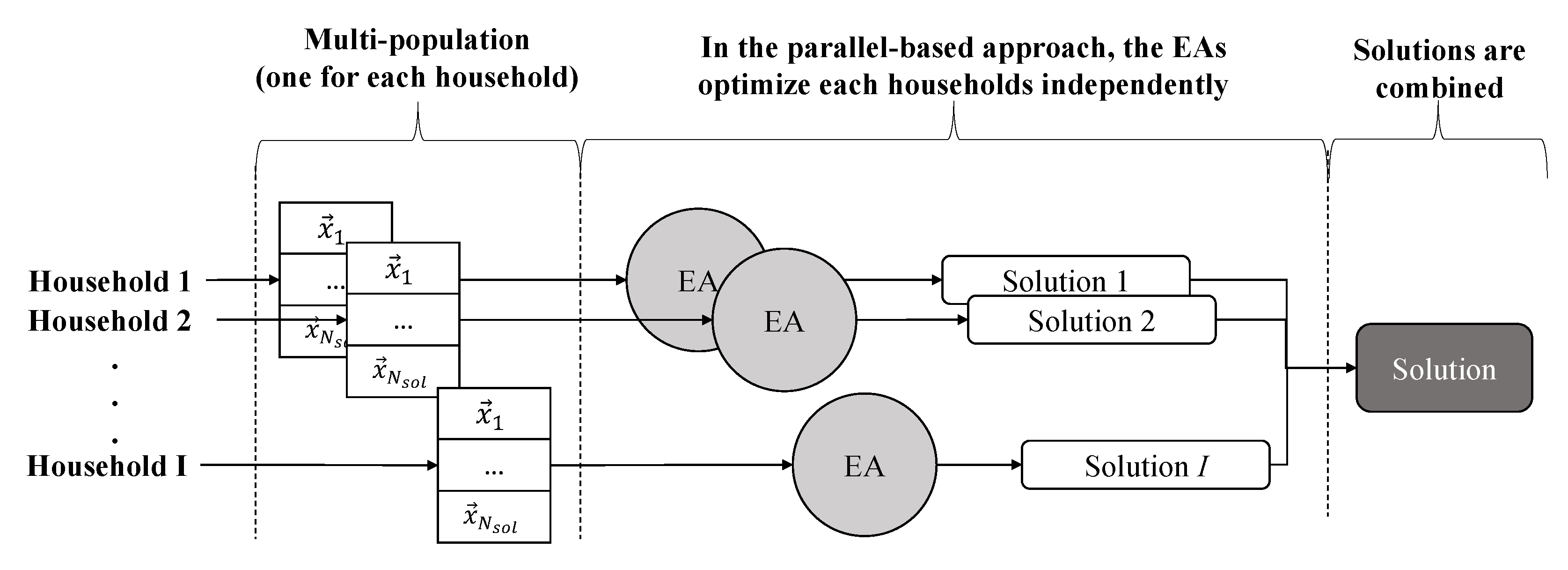
• Implementation of different EAs under two optimization approaches, one based on standard evolutionary computation and a second one taking advantage of parallel computing.
• Assessment of the effectiveness of EAs and the optimization framework under a case study considering up to 20 households.

The paper is organized as follows: after the introduction in Section 1; the proposed methodology and the mathematical formulation is presented in in Section 2; Evolutionary algorithms applied in this work are introduced in Section 3; Section 4 presents the two proposed optimization approaches employed with the use of EAs to make use of parallel computing; the case study and results are provided in Section 5 and Section 6 respectively; and finally, the conclusions of this work are presented in Section 7.

2. Households Demand Response Optimization

In this section, is provided the description of the proposed optimization model, which aims to minimize the energy bill and the user discomfort. The change in the consumption pattern is considered to be a way of user discomfort. Since it is a rather complex problem to be computed at house level, the proposed methodology considers an Energy Service Provider that performs the optimization for a large set of households, and makes the results available for each one.

In each house, distributed energy resources are available, like PV generation, storage, and DR. Accordingly, each household is a prosumer (a consumer able to produce electricity), equipped with a PV and an energy storage system. Three appliances can be controlled by the optimization algorithm to reduce the consumption in periods when the electricity price is higher. For this, it is assumed that the household owns the needed control devices (e.g., plc). The PLC (Programmable Logic Controller) controller unit manages the consumption and generation resources in the houses according to the schedule received from the Energy Service Provider.

The mathematical formulation of the problem is an extension of [20] to consider up to I households (unlike the original model designed to target only one household). Thus, the formulation corresponds to a MILP model having as OF (Objective Function) Equation (1):

$$\mathrm{Minimize}OF=EnergyBill+DRCurtailmentWeight,$$

(1)

where $EnergyBill$ represents the costs of buying and selling electricity, while $DRCurtailmentWeight$ quantifies the weight of the curtailment of loads due to DR. Thus, Equation (2) represents the energy bill that households must pay due to the flow of energy exchanged with the main grid:

$$EnergyBill=\sum _{i=1}^I\left(\sum _{t=1}^T\left(P_{i,t}^{\mathrm{Grid}\mathrm{In}}\times C_{i,t}^{\mathrm{Grid}\mathrm{In}}-P_{i,t}^{\mathrm{Grid}\mathrm{Out}}\times C_{i,t}^{\mathrm{Grid}\mathrm{Out}}\right)\times \frac{1}{\Delta t}\right)+FixCos{t}_i,$$

(2)

where $P_{i,t}^{\mathrm{Grid}\mathrm{In}}$ represents the energy flow from the grid to the household, $C_{i,t}^{\mathrm{Grid}\mathrm{In}}$ represents the cost of buying energy, $P_{i,t}^{\mathrm{Grid}\mathrm{Out}}$ is the energy flow from household to the grid, $C_{i,t}^{\mathrm{Grid}\mathrm{Out}}$ corresponds to the revenue of selling energy to the grid, $\frac{1}{\Delta t}$ is a term that considers the modification of hourly values to another time interval (e.g., 15 min in this article), $FixCos{t}_i$ represents the fixed tariff costs pay by each household. $i=\{1,\dots ,I\}$ is used to identify households, and $t=\{1,\dots ,T\}$ for the periods. Notice that Equation (2) includes the sum of energy bill over all households. Therefore, minimizing this overall value corresponds to reduce the bill for each particular household. Moreover, the energy consumption/generation from households is independent, and thus, finding the minimum value for Equation (2) guarantees that the minimum possible bill for each household is obtained.

On the other hand, Equation (3) is used to calculate the weight of DR actions:

$$DRCurtailmentWeight=\sum _{i=1}^I\left(\sum _{t=1}^T\left(\sum _{l=1}^L\left(P_{i,t,l}^{\mathrm{Cut}}\times X_{i,t,l}^{\mathrm{Cut}}\times W_{i,t,l}^{\mathrm{Cut}}\right)\right)\right),$$

(3)

where $P_{i,t,l}^{\mathrm{Cut}}$ represents the energy load cuts, $X_{i,t,l}^{\mathrm{Cut}}$ are binary decision variables indicating a DR action, $W_{i,t,l}^{\mathrm{Cut}}$ represents the weight of energy cuts, $l=\{1,\dots ,L\}$ is used to represent loads available for DR.

It is important to point out, as explained in [20] that the energy bill (first term) and DR curtailment (second term) can be seen as opposite objectives in Equation (1). This is because the curtailment of loads reduces energy bills, but at the same time affects user comfort in different ways depending on user preferences. In this work, however, we decided to select the DR weights of energy cuts following a trend contrary to the buy from grid tariff to promote the use of DR when the price of energy is higher. Other assumptions and targets can be explored in future work.

Equation (4) represents the energy balance at each period:

$$P_{i,t}^{\mathrm{Grid}}=P_{i,t}^{\mathrm{Load}}+P_{i,t}^{\mathrm{Bat}}-\sum _{l=1}^L\left(P_{i,t,l}^{\mathrm{Cut}}\times X_{i,t,l}^{\mathrm{Cut}}\right)-P_{i,t}^{\mathrm{PV}},\forall i\in \{1,\dots ,I\},\forall t\in \{1,\dots ,T\},$$

(4)

where $P_{i,t}^{\mathrm{Grid}}$ represents the energy flow between grid and household, $P_{i,t}^{\mathrm{Load}}$ represents consumption from non-controllable loads, $P_{i,t}^{\mathrm{Bat}}$ corresponds to energy charge/discharge of batteries (charge or discharge) and $P_{i,t}^{\mathrm{PV}}$ represents the energy generated by PV panels.

Equation (5) is applied to obtain the flow of energy between the grid to household:

$$P_{i,t}^{\mathrm{Grid}\mathrm{In}}=P_{i,t}^{\mathrm{Grid}}\ge 0,\forall i\in \{1,\dots ,I\},\forall t\in \{1,\dots ,T\}.$$

(5)

Equation (6) is applied to obtain the energy flow from households to the grid (exported energy):

$$P_{i,t}^{\mathrm{Grid}\mathrm{Out}}=P_{i,t}^{\mathrm{Grid}}<0,\forall i\in \{1,\dots ,I\},\forall t\in \{1,\dots ,T\}.$$

(6)

Equation (7) represents the balance of the batteries for all households at all periods:

$$E_{i,t}^{\mathrm{Bat}}=E_{i,t-1}^{\mathrm{Bat}}+P_{i,t}^{\mathrm{Bat}}\times \frac{1}{\Delta t},\forall i\in \{1,\dots ,I\},\forall t\in \{2,\dots ,T\},$$

(7)

where $E_{i,t}^{\mathrm{Bat}}$ is the state of the battery of household i at period t, and $E_{i,t-1}^{\mathrm{Bat}}$ represents the previous state of the battery of household i at period $t-1$. Equation (7) is applied from the second to the last period of optimization, while $E_{i,1}^{\mathrm{Bat}}$ is an input parameter of the case study.

Equation (8) is used to represent the bounds of $P_{i,t}^{\mathrm{Grid}}$ variable:

$$P_{i,t}^{\mathrm{Gridmin}}\le P_{i,t}^{\mathrm{Grid}}\le P_{i,t}^{\mathrm{Gridmax}},\forall i\in \{1,\dots ,I\},\forall t\in \{1,\dots ,T\},$$

(8)

where $P_{i,t}^{\mathrm{Gridmin}}$ corresponds to the lower bond and $P_{i,t}^{\mathrm{Gridmax}}$ to the upper bound values of $P_{i,t}^{\mathrm{Grid}}$.

Equation (9) represents the upper bound (maximum cut capacity) for the variable $P_{i,t,l}^{\mathrm{Cut}}$:

$$P_{i,t,l}^{\mathrm{Cut}}=P_{i,t,l}^{\mathrm{Cutmax}},\forall i\in \{1,\dots ,I\},\forall t\in \{1,\dots ,T\},\forall l\in \{1,\dots ,L\}.$$

(9)

Equation (10) presents the bonds for the variable $E_{i,t}^{\mathrm{Bat}}$.

$$0\le E_{i,t}^{\mathrm{Bat}}\ge E_{i,t}^{\mathrm{Batmax}},\forall i\in \{1,\dots ,I\},\forall t\in \{1,\dots ,T\},$$

(10)

where $E_{i,t}^{\mathrm{Batmax}}$ are the upper bound of variables $E_{i,t}^{\mathrm{Batmax}}$.

Equation (11) presents the bound for the variable $P_{i,t}^{\mathrm{Bat}}$:

$$-P_{i,t}^{\mathrm{Batdch}}\le P_{i,t}^{\mathrm{Bat}}\ge P_{i,t}^{\mathrm{Batch}},\forall i\in \{1,\dots ,I\},\forall t\in \{1,\dots ,T\},$$

(11)

where $-P_{i,t}^{\mathrm{Batdch}}$ and $P_{i,t}^{\mathrm{Batch}}$ are the lower and upper bounds of the variable $P_{i,t}^{\mathrm{Bat}}$.

Equation (12) represents the bounds for the variable $X_{i,t,l}^{Cut}$.

$$X_{i,t,l}^{Cut}=\left\{\begin{array}{c}1\hfill \\ 0\hfill \end{array}\right.,\forall i\in \{1,\dots ,I\},\forall t\in \{1,\dots ,T\},\forall l\in \{1,\dots ,L\},$$

(12)

where variable $X_{i,t,l}^{Cut}$ can takes the value of ‘1’ when the cut is active and the ‘0’ when the cut is not active.

3. Evolutionary Computation

EC (Evolutionary Computation) is one of the three pillars of computational intelligence (along with artificial neural networks and fuzzy systems). EC includes a set of algorithms for optimization inspired in biological and evolutionary processes [21]. In fact, there are in the literature now a huge set of algorithms available for optimization, but in general, they can be grouped in some popular categories such as EA, SI (Swarm Intelligence), nature-inspired algorithms, natural computation, etc.

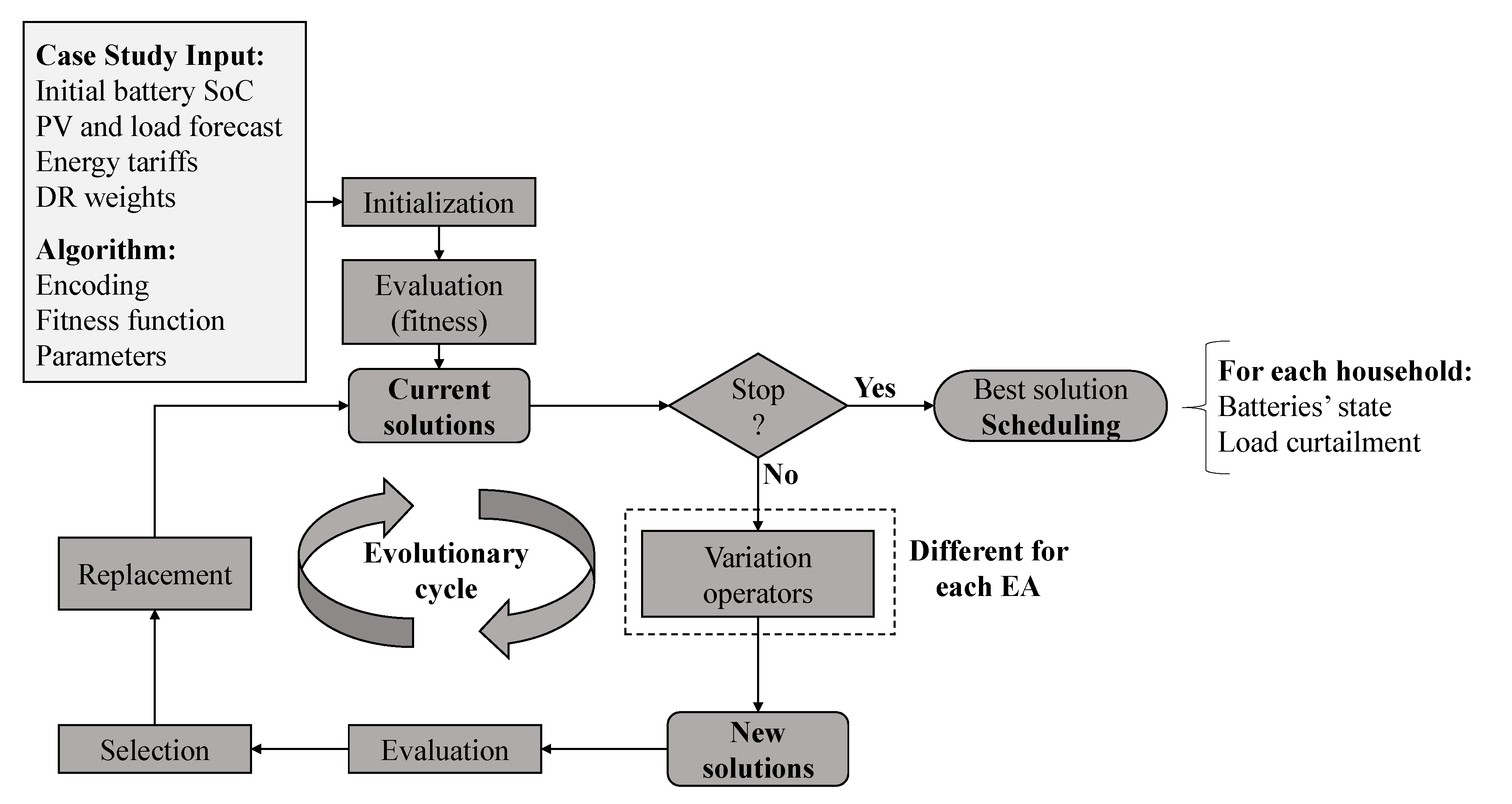
In this paper, we focus our attention in a class of algorithms that share some common mechanisms. This choice eases the experimental analysis since a fair comparison can be performed between the algorithms. Figure 1 illustrates the evolutionary mechanism employed by the selected EAs. Thus, in a first stage, an encoding of solutions and a fitness function are defined for a particular problem. The EAs act over an initial set of candidate solutions encoded as vectors (i.e., a population) that is iteratively updated through generations. The way in which new solutions are created from the initial population is what distinguish each EAs (i.e., each of the selected EAs has its own variation operator). Solutions’ performance is measured by the fitness function, and at each generation, solutions with inferior performance are replaced by the new solutions with better performance. It is empirically proved that by the principles of natural selection (or artificial selection in this case), the population will gradually evolve towards an optimal fitness value.

We describe the solution encoding and fitness function shared by the selected EAs in Section 3.1. After that, a brief description of the chosen algorithms is provided in Section 3.2.

3.1. Solution Encoding and Fitness

The optimization problem searches for the optimal scheduling of charging and discharging cycles of batteries and the choice of which loads are used for DR curtailment, for each user (as stated in Section 2).

Therefore, the selected encoding should include all the information to validate a solution, and it is very similar to that used in [20], but generalized for I users. Figure 2 shows the structure of a given solution in our framework. The solution first include continues variables representing the charging/discharging state (positive for charging, and negative for discharging) of the users’ battery, at all periods t, for each user i. Therefore, this set includes $T\times I$ variables Then, a second set of binary variables is used to indicate a cut action in all load l (‘1’ if load l is curtailed, and ‘0’ if not), at all periods t, for each user i. Therefore, this second set includes $L\times T\times I$ binary variables. In general, a complete given solution to the problem is of dimension $D=T\times I\times (1+L)$. The variables are bounded by:

$$\overrightarrow{xlb}=\{-P_{i,t}^{\mathrm{dchmax}},X_{i,l,t}^{\mathrm{cutmin}}\},i=\{1,\dots ,I\},t=\{1,\dots ,T\},l=\{1,\dots ,L\},$$

(13)

$$\overrightarrow{xub}=\{P_{i,t}^{\mathrm{chmax}},X_{i,l,t}^{\mathrm{cutmax}}\},i=\{1,\dots ,I\},t=\{1,\dots ,T\},l=\{1,\dots ,L\}.$$

(14)

Thus, the EAs can generate initial populations with random candidate solutions between those bounds using a random function such as:

$${\overrightarrow{x}}_j=\mathrm{rand}(\overrightarrow{xlb},\overrightarrow{xub}),j=\{1,\dots ,N_{sol}\},$$

(15)

where $\mathrm{rand}(\overrightarrow{xlb},\overrightarrow{xub})$ generates a random solution between the bounds defined in Equations (13) and (14), and $N_{\mathrm{sol}}$ is the size of the population defined by the user.

Since the formulation includes constraints that can be difficult to optimize by the algorithms, we apply some direct repair techniques to ease the generation of feasible solutions. Equation (16) presents the direct repair mechanism employed to keep variables $E_{i,t}^{\mathrm{Bat}}$ into the allowed limits:

$$E_{i,t}^{\mathrm{Bat}}=\left\{\begin{array}{c}0,if{E}_{i,t}^{\mathrm{Bat}}<0\hfill \\ E_{i,t}^{\mathrm{Batmax}},if{E}_{i,t}^{\mathrm{Bat}}>E_{i,t}^{\mathrm{Batmax}}\hfill \\ P_{i,t}^{\mathrm{Bat}},otherwise\hfill \end{array}\right.,\forall i\in \{1,\dots ,I\},\forall t\in \{2,\dots ,T\},$$

(16)

where variable $E_{i,t}^{\mathrm{Bat}}$ represent the energy state of charge of the battery. $E_{i,t}^{\mathrm{Bat}}<0$ represents a discharge state greater than the allowed one, so that the variable is fixed to its minimum value. When $E_{i,t}^{\mathrm{Bat}}>E_{i,t}^{\mathrm{Batmax}}$, the battery has charged more energy than the allowed, thus, the value of maximum energy in the battery is fixed the maximum allowed value. After repairing the state of charge, variables $P_{i,t}^{\mathrm{Bat}}$ should also being repaired as:

$$P_{i,t}^{\mathrm{Bat}}=\left\{\begin{array}{c}{E}_{i,t}^{\mathrm{Bat}}-E_{i,t-1}^{\mathrm{Bat}},if{E}_{i,t}^{\mathrm{Bat}}<0\hfill \\ E_{i,t}^{\mathrm{Bat}}-E_{i,t-1}^{\mathrm{Bat}},if{E}_{i,t}^{\mathrm{Bat}}>E_{i,t}^{\mathrm{Batmax}}\hfill \\ P_{i,t}^{\mathrm{Bat}},otherwise\hfill \end{array}\right.,\forall i\in \{1,\dots ,I\},\forall t\in \{2,\dots ,T\}.$$

(17)

Notice that variable $P_{i,t}^{\mathrm{Bat}}$ is repaired following the same conditions of Equation (16). This procedure guarantees feasible solutions, helping in the iterative process of the EAs.

Since the encoding has been designed to include all information needed to evaluate the mathematical model from Section 2, the fitness function is taken directly from Equation (1) including penalties due to the possibility of generate infeasible solutions. Therefore, the fitness value includes the energy bill (costs and revenues), fixed costs, and DR curtailment weight off all users plus penalties:

$$Fitness({\overrightarrow{x}}_j)=f({\overrightarrow{x}}_j)+p_{\mathrm{function}}({\overrightarrow{x}}_j),$$

(18)

where $f({\overrightarrow{x}}_j)$ is equivalent to Equation (1), and $p_{\mathrm{function}}({\overrightarrow{x}}_j)$ is a function that returns a penalty value associated with the violation of the limits of variable $P_{i,t}^{\mathrm{Grid}}$ for each user i at each time t, defined as:

$$p_{\mathrm{function}}({\overrightarrow{x}}_j)=\sum _{i=1}^I\sum _{t=1}^T{\rho }_{i,t},$$

(19)

$${\rho }_{i,t}=\left\{\begin{array}{c}0-P_{i,t}^{\mathrm{Grid}},\mathrm{if}(P_{i,t}^{\mathrm{Grid}}<0)\hfill \\ P_{i,t}^{\mathrm{Grid}}-P_{i,t}^{\mathrm{Gridmax}},\mathrm{if}(P_{i,t}^{\mathrm{Grid}}>P_{i,t}^{\mathrm{Grid}\min })\hfill \\ 0otherwise\hfill \end{array}\right.,$$

(20)

where ${\rho }_{i,t}$ is a penalty factor related to the limits of variable $P_{i,t}^{\mathrm{Grid}}$. Notice that direct repair methods are used to avoid as much as possible violations of constraints (see direct repair methods in [20]), yet, due to the stochastic nature of EAs, infeasible solutions may arise for large instances (as the result section shows).

3.2. EAs Used for DR of Households

Now that we defined the encoding of individuals and the fitness function, we apply EAs following the scheme from Figure 1 to solve the problem. In this paper, we apply DE and two of its variants hyde and HyDE (Hybrid Differential Evolution) (due to its success in many applications and easy implementation [22]), an improved version of the well-known PSO, and the vs [23]. In the following subsections, we provide a brief description of the algorithms, and their variation operators that distinguish each of them.

3.2.1. Differential Evolution

DE uses a Pop (Population) of individuals ${\overrightarrow{x}}_{j,i,G}=[x_{1,i,G},\dots ,x_{D,i,G}]$, where G is the number of iterations, $i=[1,\dots ,NP]$ is the index of individuals in the population, and $j=[1,\dots ,D]$ is the index for the variables to optimize. In the initialization stage, $NP$ solutions are generated randomly within lower and upper ranges $\overrightarrow{xlb}$ and $\overrightarrow{xub}$. In the standard form of DE, the so-called DE/rand/1 algorithm, new solutions are created applying a mutation and recombination operator defined by:

$${\overrightarrow{m}}_{i,G}={\overrightarrow{x}}_{r1,G}+F({\overrightarrow{x}}_{r2,G}-{\overrightarrow{x}}_{r3,G}),$$

(21)

$${\overrightarrow{t}}_{j,i,G}=\left\{\begin{array}{cc}{\overrightarrow{m}}_{i,G}\hfill & \mathrm{if}({\mathrm{rand}}_{i,j}[0,1]<\mathrm{Cr})\vee (j=\mathrm{Rnd})\hfill \\ {\overrightarrow{x}}_{j,i,G}\hfill & \mathrm{otherwise}\hfill \end{array}\right.,$$

(22)

where ${\overrightarrow{x}}_{r1,G},{\overrightarrow{x}}_{r2,G},{\overrightarrow{x}}_{r3,G}\in \mathrm{Pop}$ are three random individuals from the Pop, mutually different from each other. F and $Cr$ are the mutation and recombination parameters of DE, usually set in the range $[0,1]$. The fitness function, (i.e., Equation (18)), is used to evaluate the performance of new individuals. An elitist selection procedure is applied in DE by replacing solution with worse performance than the new generated ones. A detailed explanation of DE can be found in [24,25].

3.2.2. Hybrid Adaptive DE

HyDE is a new self-adaptive version of DE proposed in [25]. The distinguish HyDE variation operator, known as “DE/target-to-$perturbe{d}_{best}$/1”, modifies the well-known DE/target-to-best/1 strategy [22] perturbing the best individual (similar to the evolutionary PSO [26]). HyDE also integrate a self-adaptive parameter mechanism (taken from the jDE (Self-Adaptive Differential Evolution algorithmm [27]). The main operator of HyDE is defined as follows:

$${\overrightarrow{m}}_{i,G}={\overrightarrow{x}}_{i,G}+F_i^1(ϵ·{\overrightarrow{x}}_{\mathrm{best}}-{\overrightarrow{x}}_{i,G})+F_i^2({\overrightarrow{x}}_{r1,G}-{\overrightarrow{x}}_{r2,G}),$$

(23)

where $F_i^1$ and $F_i^2$, are scale factors in the range $[0,1]$ independent for each individual i, and $ϵ=\mathcal{N}(F_i^3,1)$ is a random perturbation factor following a normal distribution with mean $F_i^3$ (random number in the range $[0,1]$) and standard deviation 1. $F_i^1$, $F_i^2$ and $F_i^3$ are updated at each iteration with the same rule of jDE algorithm (see Section III.B of [25]).

3.2.3. Hybrid Adaptive DE with Decay Function

HyDE-DF is an improved version of HyDE used for function optimization [28]. The main different in its operation is the incorporation of a decay function that allows a transition in the iterative process from the main operator of HyDE (Equation (23)) to the basic operator of DE (Equation (21)):

$$\begin{array}{c}{\overrightarrow{m}}_{i,G}={\overrightarrow{x}}_{i,G}+{\delta }_G·[F_i^1(ϵ·{\overrightarrow{x}}_{\mathrm{best}}-{\overrightarrow{x}}_{i,G})]+F_i^2({\overrightarrow{x}}_{r1,G}-{\overrightarrow{x}}_{r2,G})\hfill \end{array},$$

(24)

where ${\delta }_G$ is a decreasing function (from $1\to 0$) that gradually mitigates the influence towards $x_{\mathrm{best}}$, and takes advantage of the inherent DE exploitation capabilities in later stages of the evolutionary process. The decay factor at each generation G is calculated as:

$$\begin{array}{c}{\delta }_G=e^{1-1/a^2};\mathrm{with}a=(GEN-G)/GEN\hfill \end{array}.$$

(25)

${\delta }_G$ factor alleviate the premature convergence effect towards the best individual in the population (i.e., due to the term $F_i^1(ϵ·{\overrightarrow{x}}_{best}-{\overrightarrow{x}}_{i,G})$). Such transition also allows an enhance exploration phase in the early stages of evolution, and improves exploitation in later stages of the optimization. HyDE-DF achieved third place (out of 36 algorithms) in the 100-digit challenge at CEC/GECCO 2019 [29].

3.2.4. PSO-LVS

PSO [20] belongs to the class of SI, in which particles (solutions to the problem) coordinate their actions by modifying their position towards the optimum value. Particles are evaluated in the fitness function and improve their position in each iteration using the following variation operator:

$$\overrightarrow{x_{j,i,G}}=\overrightarrow{x_{j,i,G-1}}+\overrightarrow{v_{j,i,G}},$$

(26)

$$\overrightarrow{v_{j,i,G}}=w_G·\overrightarrow{v_{j,i,G-1}}+c{1}_G·rand()·(P_i^{\mathrm{best}}-\overrightarrow{x_{j,i,G-1}})+c{2}_G·\mathrm{rand}()·(G^{\mathrm{best}}-\overrightarrow{x_{j,i,G-1}}),$$

(27)

where $\overrightarrow{v_{j,i,G}}$ represents the velocity vector, $w_G$ is the inertia weight, $c{1}_G$ and $c{2}_G$ are the are acceleration coefficients for personal and global component, $\mathrm{rand}()$ is a uniformly distributed random number, $P_i^{\mathrm{best}}$ is the historical best position obtained by particle i while $G^{\mathrm{best}}$ is the population historical best position obtained by the swarm.

PSO-LVS (PSO with Local Vortex Search) (Equation (28)) is a variant of PSO developed by the authors that includes a local search based on the VS algorithm. The movement of PSO-LVS is therefore obtained by following equation:

$$\overrightarrow{x_{j,i,G}}=\left\{\begin{array}{c}\overrightarrow{x_{j,i,G}}=\overrightarrow{x_{j,i,G-1}}+\overrightarrow{v_{j,i,G}}if,\mathrm{rand}()\le P^{{\mathrm{PSO}}_G}\hfill \\ p(\overrightarrow{m}/\mu ,\Sigma )=\frac{1}{\sqrt{{(2\pi )}^d\left|\Sigma \right|}}\exp \left\{-\frac{1}{2}{(\overrightarrow{x}-\mu )}^G{\Sigma }^{-1}(\overrightarrow{x}-\mu )\right\}otherwise,\hfill \end{array}\right.$$

(28)

where $P^{{\mathrm{PSO}}_G}$ is a probability factor that switch between PSO standard equation and VS. Another difference is that $\mu$ in Equation (29) is replaced by $G^{\mathrm{best}}$. In addition, $P^{{\mathrm{PSO}}_G}={0.9}^{\frac{G}{8}}$ is a probability that decreases in function of the number of generations. With this method, it is expected the execution of LVS (Local Vortex Search) in later stages of the iterative process.

3.2.5. Vortex Search

VS is classified as a single-solution-based metaheuristic, although it has an analogous framework to the EAs selected for this study. In each iteration, N given number of neighbor solutions are generated using a multivariate Gaussian distribution around the initial solution using:

$$p(\overrightarrow{m}/\mu ,\Sigma )=\frac{1}{\sqrt{{(2\pi )}^d|\Sigma |}}\exp \left\{-\frac{1}{2}{(\overrightarrow{x}-\mu )}^G{\Sigma }^{-1}(\overrightarrow{x}-\mu )\right\},$$

(29)

where d represents the dimension, $\overrightarrow{x}$ is the $d\times 1$ vector of a random variable, $\mu$ is the $d\times 1$ vector of sample mean (center), and $\Sigma$ is the covariance matrix. The N solutions generated with this function are evaluated in the fitness function, and the best solution replaces the initial single-solution. The radius of search is gradually reduced during the iterative process, favoring exploitation capabilities in the final iterations. This process is iterative repeated until a stop criterion is achieved [23].

4. Non-Parallel and Parallel-Based Approaches

In this paper, given the nature of the mathematical formulation, and the independence of variables between households, we propose two approaches to use the EAs. In the first approach illustrated in Figure 3, so-called non-parallel approach, all variables are combined in a single encoding (explained in Section 3.1). Thus, the EAs use their variation operators over the whole set of variables, until a stop criterion is achieved. This is the typical form in which an EA is applied to solve a given problem.

However, the problem formulation assume that each household scheduling is independent from each other, since their resources are individual and not shared among them. Thus, in the second approach illustrated in Figure 4, variables are divided in groups corresponding to each household. After that, multi-populations are generated and optimized independently by a chosen EA. The independent solutions are combined in a post-optimization stage, to calculate the total costs of all households. While the solution returned by both approaches is equivalent, results show that breaking the groups of variables into sets corresponding to each household in fact improves the performance of the EAs. In addition, the parallel-based approach can make use of distributed computing, running in parallel different EAs and improving convergence times.

5. Case Study

We design a case study to evaluate our framework considering households representing prosumers complying with actual Portuguese legislation, which allows small producers (consumers with local generation) to use their energy to satisfy their own load needs, and inject excess of energy to the grid. We assume that households are equipped with PV panels with a maximum power capacity of 7.5 kW and a battery unit belonging to one of the four models showed in

Table 1. Battery models used for the case study, taken from [30].

	${\mathit{P}}^{\mathbf{chmax}}$	$-{\mathit{P}}^{\mathbf{dchmax}}$	${\mathit{E}}^{\mathbf{Batmax}}$
Laboratory battery used in [20]	1.5 kW	−1.5 kW	12 kWh
Tesla Powerwall	5 kW	−5 kW	13.5 kWh
Alpha Smile	2.87 kW	−2.87 kW	14.5 kWh
Sonnen	3.3 kW	−3.3 kW	15 kWh

(distributed randomly within the households). In addition, households equipped with controllable loads can reduce 10% on average of their total consumption.

For consumption and PV generation, two sample power profiles were used to generate data of residential households. The profiles were built using real open datasets available at PES ISS website [31]. With these base profiles, up to 20 households’ data was generated using a randomized function with a uniform distribution, ±25% around the base profiles.

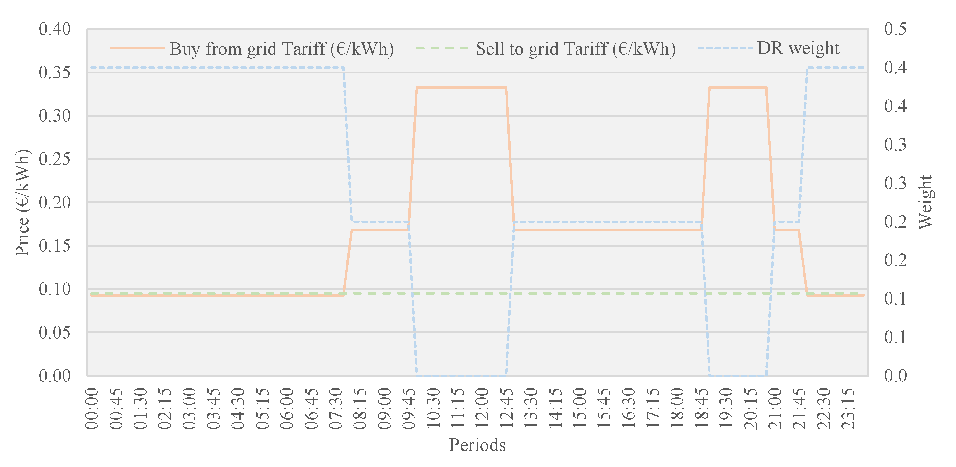
Figure 5 shows the retail tariffs and PV generation of the base profiles. We assume that households have a power supply contract with a given retailer of 11 kW characterized by three different periods: peak (0.33 EUR/kWh), intermediate (0.16 EUR/kWh), and off-peak (0.093 EUR/kWh). We also consider a feed-in tariff of 0.095 EUR/kWh and a DR weight with a trend contrary to the buy from grid tariff, i.e., promoting the use of dr when the price of energy is higher (these weights are applied to the second term of Equation (1)). Tariffs are based on real values of a Portuguese retailer.

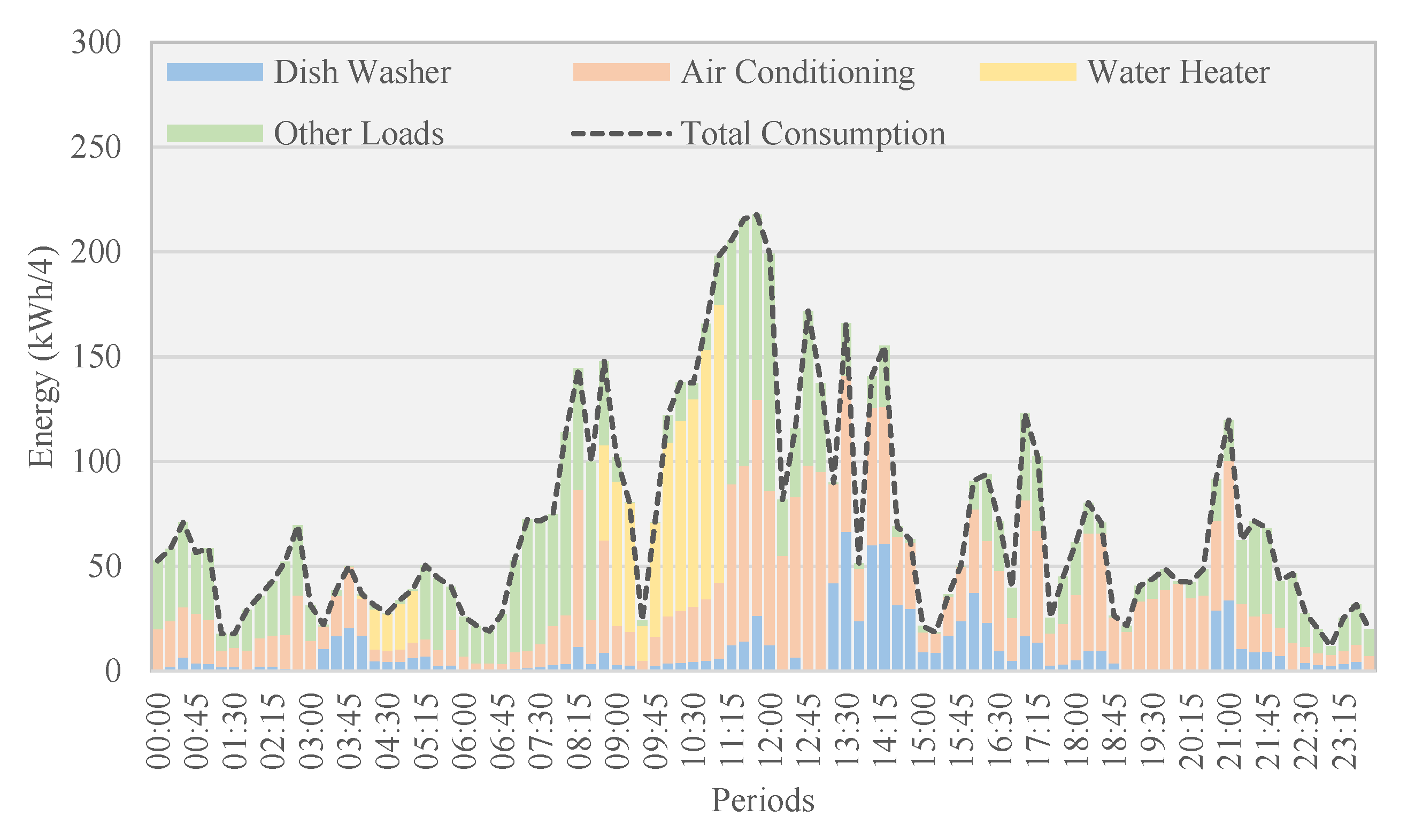
Figure 6 shows the aggregated consumption profiles of 20 households. Notice that the aggregated profile correspond to a typical profile since data from households is generated following base profiles, which in practice might not be the case. However, this paper is focused on the performance of EAs rather than the impact in the diversity of consumers. Further studies can be done considering households with diverse characteristics and their impact in costs and DR curtailment. 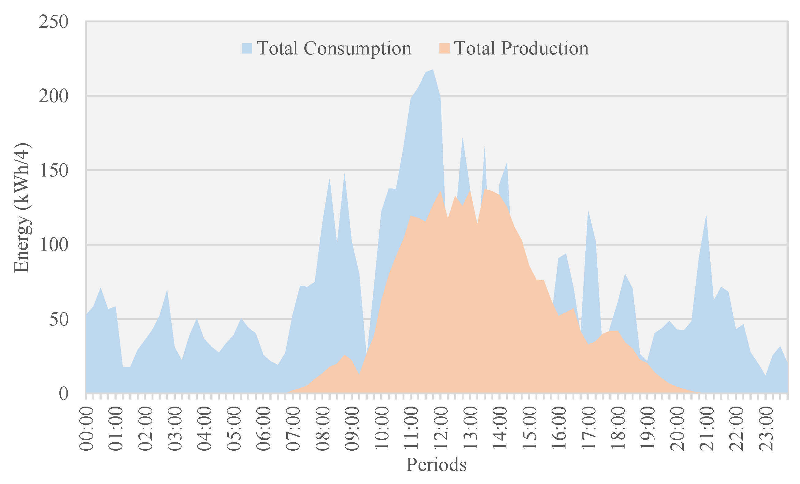Figure 7 the total aggregated consumption and generation of 20 households. Finally, input values of variables for each household are summarized in

Table 2. Input variables of the problem. Values are applied to each household.

Parameter	Variable	Value	Units
Maximum power injected to the grid	$P_{i,t}^{\mathrm{Gridmax}}$	5.1	kW
Maximum power required from grid	$P_{i,t}^{\mathrm{Gridmin}}$	1000	kW
Maximum battery capacity	$E_{i,t}^{\mathrm{Batmax}}$	12, 13.5, 14.5, 15	kW
Battery charge/discharge rate	$B_{i,t}^{\mathrm{Batch}}/B_{i,t}^{\mathrm{Batdch}}$	1.5, 5, 2.87, 3.3	kWh
Initial state of charge of batteries	$E_{i,1}^{\mathrm{Batmax}}$	0	kWh
PV maximum generation capacity	$P_{i,t}^{\mathrm{PV}}$	7.5	kW
Total Periods	T	96	-
Total of controllable loads	L	3	-
Total of batteries	B	1	-
Total of PV units	-	1	-
Adjust parameter *	$\Delta t$	4	-

* 1The factor of 4 is used since there are four 15-min periods in an hour.

6. Results

We present the results of our methodology applied to the case study of Section 5. The experiments were implemented using MATLAB2018a, in a computer with Intel Xeon(R) E5-2620v2@2.1 GHz processor with 16GB of RAM running Windows 10. All the algorithms were run for 30 times (given the stochastic nature of eas), so the reported results correspond to the average of those runs.

We perform four different experiments based on the number of households and the ea optimization approach.

Table 3. Available equipment in houses for analyzing the impact of storage and dr.

Case	Two Households	20 Households	Non-Parallel	Parallel-Based
C1	✓		✓
C2	✓			✓
C3		✓	✓
C4		✓		✓

show the four cases, identified by the letter C1-C4, related to the experiments. C1 is designed to assess the selected eas under the non-parallel approach considering two households. C2 also considers two households but under the parallel-based approach. C3 and C4 assess eas under non-parallel and parallel-based approaches respectively, but considering 20 households.

The parameters for each tested ea were selected following the recommendation of previous studies. Therefore, for de, the mutation factor and recombination constant (F and $Cr$) were set to 0.5 and 0.9 respectively [32]. hyde and HydE-DF [25] are a self-adaptive parameter versions but initial values for $F^i$ and $Cr$ where set to 0.5. For PSO-LVS the $w_G$ inertia weight is linearly decreasing with the number of iterations between 0.9 and 0.4 [33]. The constants $c{1}_G$ is set 0.5 and $c{2}_G$ set 1.8. For variables boundary control Bounce Back method is used. VS algorithm does not have any parameter to configure [23]. To make a fair comparison, all the algorithms used a population of 20 initial solutions and run for 4e3 iterations.

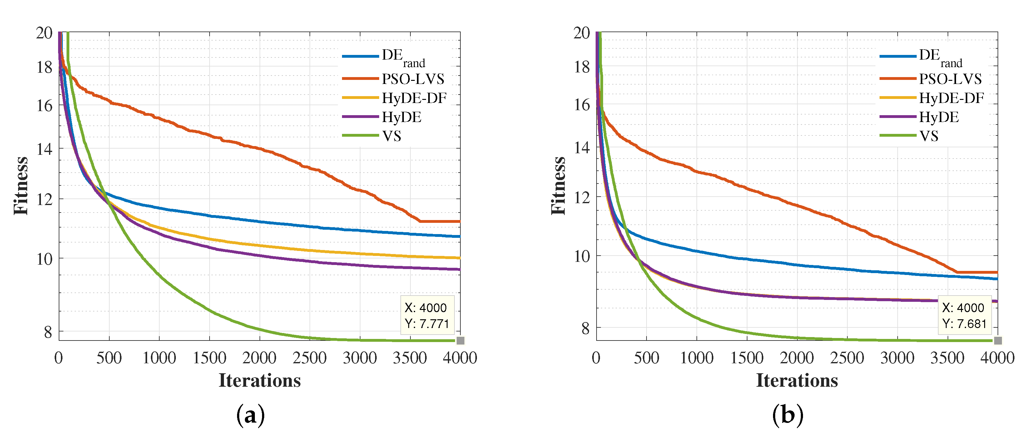
Figure 8 shows the convergence of the tested algorithms considering the two players and the non-parallel and parallel-based approaches (C1 and C2 cases). It can seem that VS presents the best convergence performance in both cases. HyDE-DF and HyDE show similar performance (in fact, convergence lines are overlapped in Figure 8b, which indicates that the improvements incorporated in HyDE-DF (that showed remarkable performance in the 100-digit challenge [29]) have almost no impact solving the proposed problem. Overall, the parallel-based approach seems to slightly improve the performance of all algorithms, without modifying the overall ranking of them. In fact, VS algorithm obtains a similar final valor.

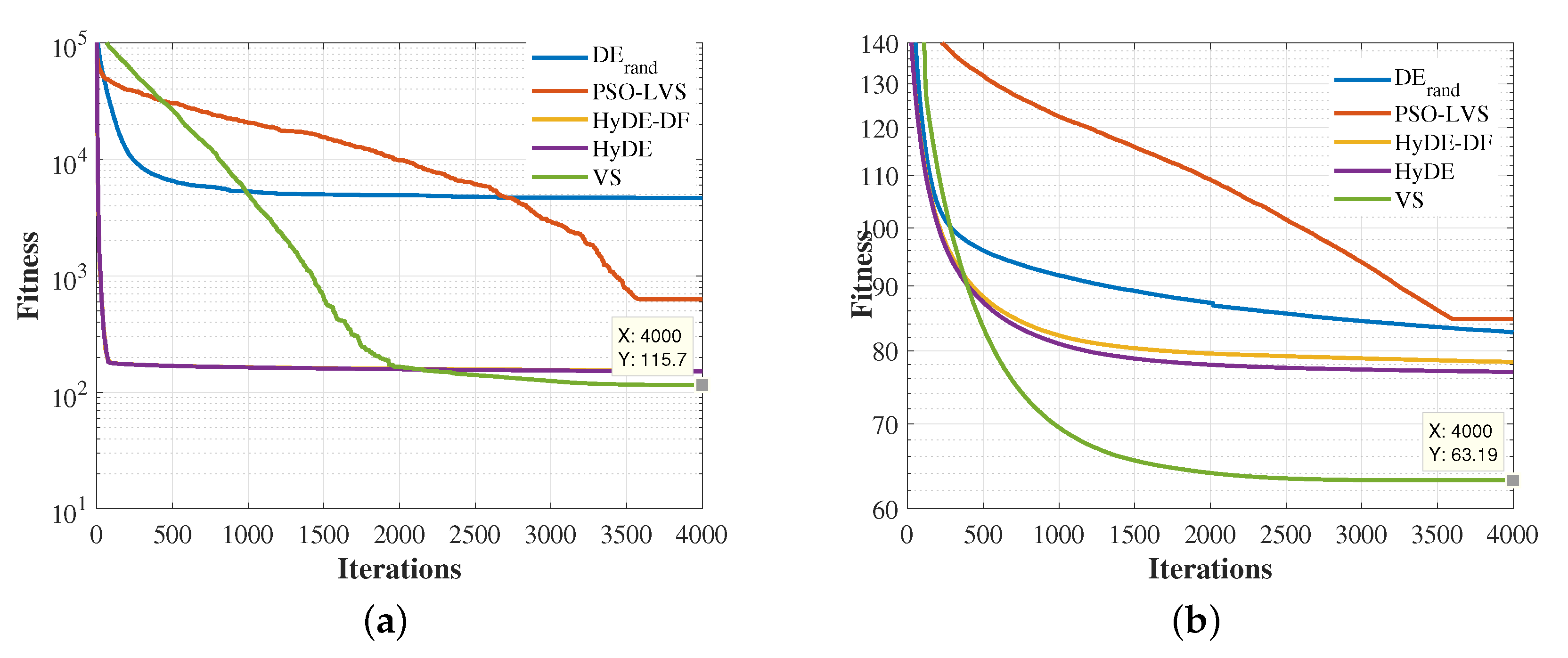
Figure 9 shows the results when increasing the number of players to 20 (C3 and C4 cases). In this case, while the non-parallel approach degrades the convergence performance of all EAs, the parallel-based approach keep the convergence performance and increasing only the final fitness value related with the cost of more households (see for instance Figure 8b and Figure 9b). In summary, the parallel-based approach can help EAs in finding quality solutions for even large instances of the problem. Also, notice that $D{E}_{\mathrm{rand}}$ and PSO-LVS, apart from showing the worse performance, switch their convergence behavior when the non-parallel approach is used and the number of players increases (see for instance Figure 8a and Figure 9a). That result shows evidence of their lack of robustness, since their performance should not be affected by the increase of the number of players.

We also analyze the average fitness and associated costs/revenues obtained by the EAs in all the cases.

Table 4. Case C1: Fitness value and associated costs considering two households and non-parallel EAs.

	Fitness		Time	Costs	Revenues	Fixed	Daily	Monthly	DR	Imp
	mean	std	(min)	(€)	(€)	Costs (€)	Bill * (€)	Bill ** (€)		(%)
DE	10.69	0.46	1.16	9.29	−2.75	1.02	7.56	226.94	1.68	4.52
PSO	11.19	0.44	1.14	10.29	−2.11	1.02	9.21	276.25	0.75	0.00
HyDE	9.94	0.78	1.43	10.13	−1.21	1.02	9.95	298.43	0.00	11.23
HyDE-DF	9.59	0.83	1.42	9.78	−1.18	1.02	9.62	288.74	0.00	14.35
VS	7.77	0.08	1.48	9.09	−2.43	1.02	7.69	230.65	0.08	30.57

* Daily bills are calculated as buy Costs − sell Revenues + fixed Costs. ** Monthly bill on average considering 30 days.

,

Table 5. Case C2: Fitness value and associated costs considering two households and parallel-based EAs.

	Fitness		Time	Costs	Revenues	Fixed	Daily	Monthly	DR	Imp
	mean	std	(min)	(€)	()	Costs (€)	Bill * (€)	Bill ** (€)		(%)
DE	9.30	0.34	1.03	9.34	−2.80	1.02	7.56	226.84	0.54	2.03
PSO	9.49	0.22	1.05	9.79	−2.04	1.02	8.77	263.21	0.28	0.00
HyDE	8.64	0.41	1.31	9.66	−1.97	1.02	8.72	261.55	0.00	8.97
HyDE-DF	8.67	0.46	1.30	9.53	−1.67	1.02	8.88	266.46	0.00	8.68
VS	7.68	0.03	1.36	9.27	−2.62	1.02	7.67	230.18	0.00	19.06

* Daily bills are calculated as buy Costs − sell Revenues + fixed Costs. ** Monthly bill on average considering 30 days.

,

Table 6. Case C3: Fitness value and associated costs considering 20 households and non-parallel EAs.

	Fitness		Time	Costs	Revenues	Fixed	Daily	Monthly	DR	Imp
	mean	std	(min)	(€)	(€)	Costs (€)	Bill * (€)	Bill ** (€)		(%)
DE	4672.93	2362.42	3.98	104.67	−35.33	10.24	79.57	2387.22	4.31	-
PSO	626.70	602.42	3.70	147.50	−19.79	10.24	137.94	4138.31	2.03	-
HyDE	149.45	3.86	4.93	150.40	−11.17	10.24	149.47	4484.04	0.02	0.00
HyDE-DF	148.58	4.26	4.93	150.59	−11.99	10.24	148.84	4465.34	0.03	0.58
VS	115.69	3.95	5.51	83.17	−33.48	10.24	59.93	1797.81	2.57	22.59

* Daily bills are calculated as Buy costs − Sell Revenues + Fixed Costs. ** Monthly bill on average considering 30 days.

and

Table 7. Case C4: Fitness value and associated costs considering 20 households and parallel-based EAs.

	Fitness		Time	Costs	Revenues	Fixed	Daily	Monthly	DR	Imp
	mean	std	(min)	(€)	()	Costs (€)	Bill * (€)	Bill ** (€)		(%)
DE	82.72	2.24	9.69	86.54	−31.95	10.24	64.83	1944.86	0.82	2.36
PSO	84.72	0.90	9.60	92.32	−25.01	10.24	77.55	2326.41	0.39	0.00
HyDE	77.83	2.40	11.87	89.79	−21.38	10.24	78.65	2359.42	0.02	8.13
HyDE-DF	76.77	2.24	11.77	89.21	−20.02	10.24	79.43	2382.86	0.00	9.38
VS	63.19	0.26	12.31	84.29	−31.53	10.24	63.00	1889.92	0.01	25.41

* Daily bills are calculated as Buy costs − Sell Revenues + Fixed Costs. ** Monthly bill on average considering 30 days.

present the average values of fitness, time, daily bill and DR curtailment, as well as the calculation of fitness percentage improvement, taking as reference the worst fitness value in each case. Table 4 shows the average results obtained in the case C1. First thing to observe is that VS presents the lower fitness value, but also the higher optimization time. However, all EAs present similar optimization times (ranging from 1.15 to 1.5 min). Regarding costs/revenues, it is interesting to note that despite VS obtains the best fitness value, its daily costs (Daily Bill column in the table) is slightly higher than that obtained by DE. This is explained by column DR curtailment, which shows that DE activates DR curtailment in a higher degree than the other algorithms. While this is beneficial for the energy bill, it also represents a higher number of interruption of loads during the day, which can impact user comfort in some degree. Notice that DR curtailment in the formulation is not a monetary cost, but rather a weight associated with the interruption of loads. Future work can study the multi-objective nature of the formulation to optimize both terms in Equation (1) simultaneously. Finally, VS achieved the best performance with an improvement of around 30 % compared to PSO (worst algorithm for case C1).

Table 5 presents the results corresponding to case C2. It can seem that the general trends, as reported in case C1 results, are followed by the EAs when low number of households are considered. Mean Fitness and overall daily bills are slightly improved. Optimization times are equivalent, but it should be taken into account that column Time reflects the sum of the independent optimization of both households. Such optimizations can be done in parallel since are independent, reducing the optimization time by half, while obtaining better results regarding fitness and daily bills. In case C2, VS again achieved the best performance with an improvement of around 20 % compared to PSO (worst algorithm for case C2).

When the number of households increases, different conclusions are achieved. Table 6 and Table 7 present the results corresponding to cases C3 and C4. The first thing to remark are the high fitness value reported by DE and PSO-LVS in case C3. Such high values are associated with the inability of both algorithms to find feasible solutions (i.e., the solutions include penalties explained in Equation (19)). Therefore, it is confirmed that these two algorithms are very sensitive to the increase in the number of households when the non-parallel approach is used. Such situation is corrected by the parallel-based approach, as Table 7 shows. In fact, the advantage of using this approach is stressed concerning fitness and daily bill values when the number of households is increased. Notice that since optimization times in the parallel-based approach correspond to the sum of independent optimizations, increasing the number of households affect notably the optimization times (see column Time of Table 7). However, such independent optimization can be performed in parallel reducing the time considerable depending the available parallel computing capacity. For instance, in MATLAB using four workers in the parallel pool (four parallel optimizations), the optimization time can be reduced by a factor of 5. Overall, VS achieved the best performance in both cases, with an improvement of around 22% compared to HyDE in case 3 (worst algorithm without considering DE and PSO due to reported infeasible solutions) and around 25% in case C4 compared to PSO.

7. Conclusions

In this paper, a different EAs are used to solve an optimization problem considering households with PV-battery systems and DR. Taking advantage of the independence of variables between households, two optimization approaches, non-parallel and parallel-based, are proposed. Results showed that EAs using the parallel-based approach provide solutions with better fitness value when the number of households increases. It was demonstrated that the direct application of an EA to larger instances of the problem (the non-parallel approach) has poor convergence capabilities (despite being very efficient when applied to one or two households). On the other hand, the proposed parallel-based approach showed excelled performance even when increasing the number of households. It is important to notice that the parallel-based approach is only valid for a framework as the one assumed in this work (which is actually a very likely real scenario due to the possible resistance of households to share data or equipment between peers), so changing such conditions might require a hybrid non-parallel and parallel approach. Overall, VS algorithm overcomes other tested EAs when using both optimization approaches. In fact, improvements of 30.57 % for case C1, 19.06 % for case C2, 22.59 % for case C3, and 25.41 % for case C4, were achieved with VS (best performance) compared to PSO (worst performance). Another advantage of the parallel-based approach is related to the possibility of using parallel computing to reduce optimization times while obtaining solutions with good quality. From the practical point of view, in this work we have envisaged the involvement of an Energy Service Provider that performs the optimization of households equipped with distributed energy resources (like PV generation, storage, and demand response) and the needed control devices. In this way, several business models can be explored by the Energy Service Provider within this framework. For instance, the service provider can charge a fee or commission from the total bill reduction achieved by the households, or receive incentives from upper level actors (such as the DSO) for the reduction of peak demand through DR. These two options, and other business model possibilities exploring the use of available infrastructure for practical implementations can be explored in future work. Another line of research for future work is related to the mathematical model. In this work, energy bill and DRdr curtailment are combined into a single objective formulation despite being terms that can be optimized in function of user preferences. Thus, multi-objective optimization versions of EAs can be employed to find Pareto optimal solutions. Moreover, a relation between DR curtailment and user comfort was not explicitly defined in this study, so another line of research can be followed concerning the modelling of user comfort. Finally, the practical implementation of EAs is also worth to be explored in future works. The parallel-based approach uses a multi-population similar to that used by coevolutionary algorithms, so testing those kinds of algorithms and their performance in this problem since a good research avenue. In addition, in this study the parallel-based approach was implemented sequentially, so optimization times reflect the sum of all independent optimizations. In a future study, the implementation of an actual parallel platform can be proposed to handle larger instances of the problem and assess the reaches and scalability of the approach.