Increasing Compressed Gas Energy Storage Density Using CO₂–N₂ Gas Mixture

Abstract

This paper demonstrates a new method by which the energy storage density of compressed air systems is increased by 56.8% by changing the composition of the compressed gas to include a condensable component. A higher storage density of 7.33 MJ/m³ is possible using a mixture of 88% CO₂ and 12% N₂ compared to 4.67 MJ/m³ using pure N₂. This ratio of gases representing an optimum mixture was determined through computer simulations that considered a variety of different proportions from pure CO₂ to pure N₂. The computer simulations are based on a thermodynamic equilibrium model that predicts the mixture composition as a function of volume and pressure under progressive compression to ultimately identify the optimal mixture composition (88% CO₂ + 12% N₂). The model and simulations predict that the optimal gas mixture attains a higher energy storage density than using either of the pure gases.

1. Introduction

Energy storage is a central piece in the efforts to modernize the electric grid, reduce cost of electricity to both utilities and end users, and to enable higher penetration of renewable energy technologies. Various technologies have been invented for energy storage with different degrees of maturity. An extensive review of the available energy storage technologies, their cost, performance and maturity is presented in [1]. Large-scale electric energy storage is dominated by Pumped Storage Hydropower (PSH) with a share of approximately 99.5% of the total installed capacity worldwide on a GW basis [2]. Large-scale non-PSH electric energy storage is dominated by Compressed Air (CAES) followed closely by Lithium-ion batteries as shown in Figure 1.

PSH is a mature technology with a relatively high round-trip efficiency [3]. However, it is only economical at a scale of 100 MWe and higher [4] and it has poor expansion potential in the US since most suitable sites have already been exploited. The geographical and scale limitations of the PSH makes it unsuitable for behind the meter storage in buildings. Compressed air energy storage (CAES) is another large-scale storage that uses turbomachinery to store and retrieve energy from high-pressure reservoirs. Conventionally, CAES uses natural caverns as storage vessels. Conventional CAES is, similar to PSH, geographically limited by the availability of naturally occurring caverns [5]. Above-ground CAES, that uses pressure vessels rather than caverns, have been proposed and smaller scale systems built [4,6]. The round trip efficiency of CAES systems is in the 40–50% range [4,7]. More advanced configurations of CAES have been investigated and were claimed to have significantly higher round trip efficiencies [8]. Above-ground CAES is amenable to installations in buildings behind the meter. However, their relatively low round trip efficiency hurts their economic viability. Liquefied Air Energy Storage (LAES), similar to CAES, stores electric energy in the form of high pressure, low-temperature liquefied air. Different possible configurations of LAES systems were analyzed in [9]. The study proposed hybridizing the LAES with another energy storage technology of faster response time, such as a Lithium-ion battery, to mitigate the slow intrinsic response of LAES. Round trip efficiency in the range of 50% to 62% has been reported in the literature for LAES [10,11]. Batteries are the most ubiquitous electricity storage device due to their excellent modularity and scalability from fractional- to Mega- watt scale. Batteries have high energy density (ED) owing to the high energy levels that can be stored in chemical bonds. They have been typically manufactured with capacity in the range of few kilowatt-hours. However, recently, Megawatt-hour scale battery systems have started to emerge as an option for grid-scale energy storage. Despite their ubiquity and high energy density, battery systems still face serious challenges to their adoption for large-scale electricity storage. Batteries have limited life and deep cycling them accelerates their deterioration [4]. They require replacement every few years and they are made of hazardous chemicals. The process to dispose of them safely is environmentally and financially costly. A great deal of research and development effort has been invested in reducing the cost, increasing the lifetime, and improving management systems of grid-scale battery systems [4,12,13]. Lithium-ion batteries are so far the most mature and readily available for large-scale storage. Current research is focused on better chemistries [14,15,16] for these batteries. The Ground-Level Integrated Diverse Energy Storage (GLIDES) is a recently invented modular technology that utilizes gas compression for electric energy storage [17]. Its scalability makes it suitable for behind the meter storage in buildings as well as for grid-scale storage. GLIDES relies on hydraulic compression of gas inside a vessel to store energy. Its modularity makes it suitable for installations in urban areas where storage is most needed and real estate is limited. Effort is continuing to improve the economic potential of GLIDES by reducing its first cost and increasing its energy density to reduce the overall cost per kWh. Typically, GLIDES uses air as the compressed gas. Merely compressing air penalizes the energy density. Other inert, innocuous, inexpensive gases can vastly improve the energy density. This paper presents a vapor–liquid equilibrium model to calculate the maximum possible increase in energy density that results from replacing air with a mixture of nitrogen and carbon dioxide. The working principles of GLIDES will be presented in the methodology section followed by modeling and analysis.

2. GLIDES Working Principle

The concept, advanced configurations, and experimental evaluation of GLIDES are referenced in [18,19,20,21]. Only a brief description of the working principles of GLIDES is shown in Figure 2. Initially, the pressure vessels are charged with a gas to some initial pressure. To store energy, a positive displacement pump pushes liquid into the pressure vessels. The liquid column level inside the vessels rises and the gas is compressed, causing its pressure to increase. This process continues until the maximum allowable working pressure of the vessels is reached. To retrieve the stored energy, liquid is let out of the vessels. The liquid flows through hydraulic turbine which in turn spins an electrical generator to produce electricity.

Water was originally selected as the compression liquid because of its abundance and low-cost. Air was originally selected as the compressed gas inside the vessels. This is because air is abundant, low-cost, non-toxic, and non-flammable.

3. Methodology

The energy stored in GLIDES is from compression work that is done by a compression liquid column on a gas in a vessel and is given by:

$$\begin{array}{c}W=-{{\displaystyle \int }}_{V_0}^{V_f}P dV, V_f<V_0\end{array}$$

(1)

To maximize ED of GLIDES, one needs to either maximize the pressure, maximize the change of volume or maximize both.

In the absence of phase change, pressure rise is coupled with the change in volume under isothermal compression. In this case, the maximum ED achievable using a certain vessel is limited by the maximum allowable working pressure of the vessel. However, increasing the maximum allowable working pressure requires stronger storage vessels and more safety inspections which increases the cost of GLIDES on a kWh basis. If, on the other hand, a gas is used such that when compressed it condenses into liquid, pressure is decoupled from the change of volume under isothermal compression. Since the density of the condensed fluid is higher than its density in vapor phase, the volume that can be utilized for energy storage is increased. In this case, the maximum ED achievable is limited by the volume of the vessel and the saturation pressure of the gas under the working temperature. These two cases are illustrated in Figure 3.

An inexpensive, non-toxic, non-flammable, and readily available gas that condenses at relatively high pressure at room temperature is CO₂. Although, using CO₂ maximizes the volume of the vessel that can be utilized for energy storage, the pressure is restricted to approximately 60 bar, depending on the ambient temperature. This pressure is much lower than the existing vessel’s maximum allowable working pressure of 140 bar [21]. The goal of this study is to determine whether using a mixture of air and CO₂ can result in higher ED than using air alone. To do so, we model the process of compressing a mixture of a non-condensable gas under the working temperature and pressure (N₂) and a condensable gas (CO₂). N₂ is used to represent air to simplify the model. The model predicts the instantaneous composition of the mixture, the pressure and the volume of the gas mixture. ED is then calculated by numerically integrating the pressure over the volume bounds. The model was run parametrically to analyze the effect of the initial mole fraction and the initial pressure on the ED of the system

4. Model

A schematic of the model is shown in Figure 4. A vessel is initially charged, to a known initial pressure, with a CO₂/N₂ mixture to some known mole fraction. A liquid, mineral oil in which both N₂ and CO₂ are immiscible, is pumped into the vessels at a constant flow rate. As the liquid column rises inside the vessel, the gaseous mixture is compressed, and its pressure rises. When the partial pressure of CO₂ equals, and subsequently exceeds its saturation pressure, CO₂ starts to condense, forming liquid condensate on top of the compression liquid column. Compression is terminated when the volume of the gaseous mixture reaches less than 5% of the total volume of the vessel or until the pressure reaches 140 bar.

For simplicity, the compression process is assumed to be isothermal. This is justified because energy is stored incrementally at a slow rate. This allows sufficient time for heat to flow through the conductive walls of the pressure vessel to sustain isothermal compression. Furthermore, the analysis being presented in this paper aims to find a bounded solution for the maximum possible increase in energy density that results from using the CO₂/N₂ mixture instead of air. The CO₂ and N₂ are modeled as real gases using the Redlich–Kwong equation of state.

At any time, the volume of the compression liquid in the vessels is:

$$\begin{array}{c}{V}_{CL}=Q \Delta t\end{array}$$

(2)

And the volume of the gaseous mixture is:

$$\begin{array}{c}{V}_G=V_V-V_{CL}-V_{C{O}_2\left(L\right)}\end{array}$$

(3)

The change in the volume of the gaseous mixture in the vessel causes the pressure to rise in the vessel. The relationship between the pressure and the volume of the compressed gaseous mixture is modeled by the Redlich–Kwong equation of state:

$$\begin{array}{c}P=\frac{RT}{V_m-b}-\frac{a}{\sqrt{T} V_m\left(V_m+b\right)}\end{array}$$

(4)

where:

$$\begin{array}{c}a=0.427480 \frac{R^2{T}_c^{2.5}}{P_c}\end{array}$$

(5)

$$\begin{array}{c}b=0.086640 \frac{R{T}_c}{P_c}\end{array}$$

(6)

$$\begin{array}{c}{V}_m=\frac{V_G}{N_G}\end{array}$$

(7)

For a mixture of gases, a and b in Equation (4) are replaced by a_G and b_G that are calculated from each species’ individual a and b as follows:

$$\begin{array}{c}{a}_{ij}=\sqrt{a_i{a}_j}\end{array}$$

(8)

$$\begin{array}{c}{a}_G={\displaystyle {\displaystyle \sum }_i}{\displaystyle {\displaystyle \sum }_j}{y}_i{y}_j{a}_{ij}\end{array}$$

(9)

$$\begin{array}{c}{b}_G={\displaystyle {\displaystyle \sum }_i}{y}_i{b}_i\end{array}$$

(10)

When the partial pressure of CO₂ reaches its saturation pressure at the tank temperature (which is constant), CO₂ condenses and its mole fraction in the gaseous mixture becomes:

$$\begin{array}{c}{y}_{C{O}_2}=\frac{P_{C{O}_2}^{Sat}}{P_T}\end{array}$$

(11)

The number of moles of gaseous CO₂ is then:

$$\begin{array}{c}{N}_{C{O}_2\left(G\right)}=y_{C{O}_2} N_G\end{array}$$

(12)

The number of moles of CO₂ in liquid phase is calculated by applying the conservation of mass:

$$\begin{array}{c}{N}_{C{O}_2\left(L\right)}=N_{C{O}_2}^0-N_{C{O}_2\left(G\right)}\end{array}$$

(13)

When condensation is taking place, $N_{C{O}_2\left(G\right)}$ and $N_{C{O}_2\left(L\right)}$ are both changing with time. At the beginning of each time step, the volume (or molar volume) of the gas mixture and its pressure are unknown. To solve for them, the solution must be iterative which is computationally more expensive that an explicit solution. Besides, an iterative solution is further complicated by the discontinuity in the solution that is caused by phase change. Instead of driving the solution procedure by marching in time and starting from the change of volume, a computationally simpler approach is to solve for volume by marching in pressure. This methodology leads to a more tractable and explicit solution. The steps are detailed below and schematically in Figure 5.

We increment the total pressure every step. Because the total pressure is known, a determination is made as to whether condensation is occurring or not. If no condensation is occurring, then the total number of moles in the gaseous phase is known and equals its initial value. Equation (4) can then be solved for molar volume. A direct solution of Equation (4) is cumbersome and requires a trial and error procedure. To overcome this computational hurdle, Equation (4) is rearranged into its cubic form:

$$\begin{array}{c}{Z}^3-Z^2+\left(A-B-B^2\right)Z-AB=0\end{array}$$

(14)

where:

$$\begin{array}{c}Z=\frac{P{V}_m}{RT}\end{array}$$

(15)

$$\begin{array}{c}A=\frac{a_{G}P}{R^2{T}^{2.5}}\end{array}$$

(16)

$$\begin{array}{c}B=\frac{b_{G}P}{RT}\end{array}$$

(17)

Equation (14) is then solved for Z. The solution of this cubic equation gives three roots, two of which are imaginary, and conjugates of each other, and only one is real. The imaginary roots are discarded, and V_m is calculated from the real root using Equation (15). The volume of the gaseous mixture is:

$$\begin{array}{c}{V}_G=N_G^0 V_m\end{array}$$

(18)

If it is determined that condensation is occurring, then the mole fraction of CO₂ in the gaseous mixture is calculated from Equation (11). Since N₂ will not condense at room temperature, its number of moles in the gaseous mixture is already known and is equal to its initial value. The total number of moles of the gaseous mixture is:

$$\begin{array}{c}{N}_G=\frac{N_{N_2}}{1-y_{C{O}_2}}\end{array}$$

(19)

And the number of moles of CO₂ in the gaseous mixture becomes:

$$\begin{array}{c}{N}_{C{O}_2\left(G\right)}=N_G-N_{N_2}\end{array}$$

(20)

And the number of CO₂ moles in liquid phase is:

$$\begin{array}{c}{N}_{C{O}_2\left(L\right)}=N_G^0-N_G\end{array}$$

(21)

To calculate the volume of the gaseous mixture, Equation (14) is solved for Z and V_m is calculated from Equation (15) then the volume is calculated:

$$\begin{array}{c}{V}_G=N_G{V}_m\end{array}$$

(22)

When the termination condition, previously qualified, is reached, the ED is calculated by numerically integrating the pressure over volume using the trapezoidal integration method.

A full factorial was run that covered CO₂ initial mole fraction range from 0 to 99% with 1% increments and initial pressure range from 30 to 100 bar with 1 bar increments. Temperature of the gaseous mixture was assumed to be constant at 25 °C throughout the compression process.

Every pressure step was incremented by a fixed amount and the solution proceeded as described above assuming equilibrium between the CO₂ in the gaseous mixture and the condensed liquid. To determine an appropriate pressure increment, we investigated the effect of the pressure increment on the accuracy of the solution. Equilibrium, under isothermal condition, stipulates that the properties of the systems are a unique function of pressure. In other words, at any given pressure, there is one and only one, unique solution for the volume of the gaseous mixture, composition of the gaseous mixture and number of moles of condensed CO₂ regardless of the time elapsed between any two states. Hence, the size of the pressure increment does not affect the prediction of the aforementioned properties. It does, however, affect the error of the numerical integration. Therefore, the size of the pressure increment must be chosen so that the maximum error in the numerical integration is kept minimal. The error associated with trapezoidal numerical integration of pressure over non-equally spaced n-segments of volume is:

$$\begin{array}{c}E=\frac{{\left(V_f-V_0\right)}^3 }{12 n^2} \frac{{{\displaystyle \sum }}_{i=1}^n{P}^{″}\left(V_i\right)}{n}\end{array}$$

(23)

This formula gives the post-integration error, since it requires that the second derivative of P(V) to be known. By examining the term $\frac{{{\displaystyle \sum }}_{i=1}^n{P}^{″}\left(V_i\right)}{n}$, it is obvious that this the average of the second derivative of P(V) over the period [V₀, V_f]. An expression could be derived for this derivative analytically from Equation (24):

$$\begin{array}{c}P=\frac{ZRT}{V}\end{array}$$

(24)

It then follows that:

$$\begin{array}{c}{P}^{″}=2\frac{ZRT}{V^3}\end{array}$$

(25)

And the average of the second derivative of P(V) over [V_0, V_f] can be calculated:

$$\begin{array}{c}\frac{{{\displaystyle \int }}_{V_0}^{V_f}\frac{2ZRT}{V^3}dV}{\left(V_f-V_0\right)}=-\frac{ZRT \left(\frac{1}{V_f^2}-\frac{1}{V_0^2}\right)}{\left(V_f-V_0\right)}\end{array}$$

(26)

And Equation (23) could be re-written as:

$$\begin{array}{c}E=-\frac{{\left(V_f-V_0\right)}^3 }{12 n^2} \frac{ZRT \left(\frac{1}{V_f^2}-\frac{1}{V_0^2}\right)}{\left(V_f-V_0\right)}\end{array}$$

(27)

For every combination of initial mixture composition and initial pressure, the outcome is different since the volume bounds of the gaseous mixture are different. However, since the goal is to determine a size of pressure increment that will minimize the error, Equation (27) was solved for the worst case of V_f = 0.05 m³, V₀ = 1 m³, Z = 1, and R = 296.8 J/kg·K, which corresponds to N₂ and is higher than that of CO₂. It has been shown that a GLIDES system of the same size and same pressure bounds under investigation has ED on the order of several 10⁶ J/m³. Hence, the upper bound of the absolute error in ED was chosen as 1000 J/m³. This ensures that the error is small enough that it does not affect the result materially. For the worst case, the number of steps as calculated from Equation (27) was 52 steps. The smallest pressure range in our parametric study was 40 bar. Hence, the pressure increment size must be less than 80,000 Pa to maintain the error in ED below the chosen bound. The model was solved using pressure increments of 100 Pa to ensure better accuracy and to obtain a good graphing resolution.

5. Results and Discussion

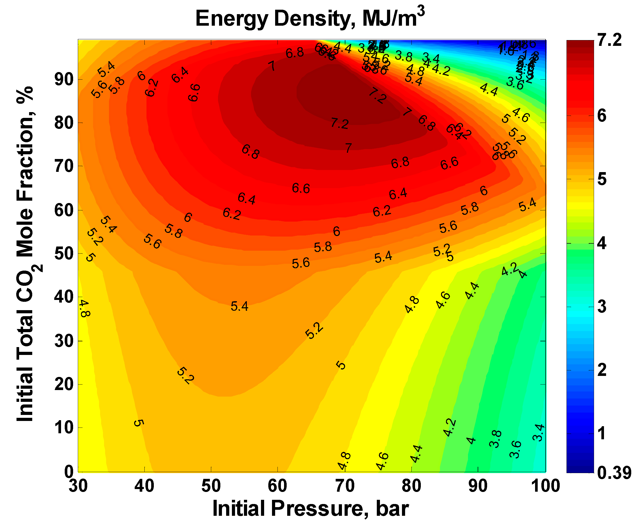
A contour plot and a surface plot of the ED for the full factorial is shown in Figure 6 and Figure 7, respectively. For any initial pressure, increasing the initial total mole fraction of CO₂ increases the ED initially till a maximum after which the ED starts to decrease. A similar trend is true for increasing initial pressure at any CO₂ initial total mole fraction. This is the manifestation of the competing effects of higher pressure versus larger utilized volume as explained in the following paragraphs. The maximum achieved ED was 7.3285 MJ/m³ and occurred at a CO₂ initial total mole fraction of 88% and an initial pressure of 73 bar.

To understand the resultant of the two competing effects, namely the initial total CO₂ mole fraction and the initial pressure, on ED, examine Figure 8 and Figure 9. Figure 8 shows the P–V diagram for the optimal initial pressure of 73 bar and three different initial total CO₂ mole fractions: 0% (pure N₂), 88% (optimal fraction), and 99% (almost pure CO₂). With no CO₂ in the system, the final pressure reaches the maximum allowable limit of 140 bar at gas volume of 52% of the total volume of the vessel. With initial total CO₂ mole fraction of 99%, the process starts at a gaseous mixture volume of approximately 23% of the total vessel volume. This is because the system initially had condensed CO₂ column, since the initial partial pressure of CO₂ was already higher than the saturation pressure at 25 °C. The process reaches the minimum allowable gaseous volume of 5% at a pressure of approximately 117 bar. With the optimal initial total CO₂ mole fraction of 88%, the process starts at the maximum possible volume, which is the total volume of the vessel, and reaches the maximum allowable pressure of 140 bar at a gas volume of approximately 15% of the total vessel volume. The optimal value maximizes both the change of the gaseous mixture volume and the final pressure simultaneously.

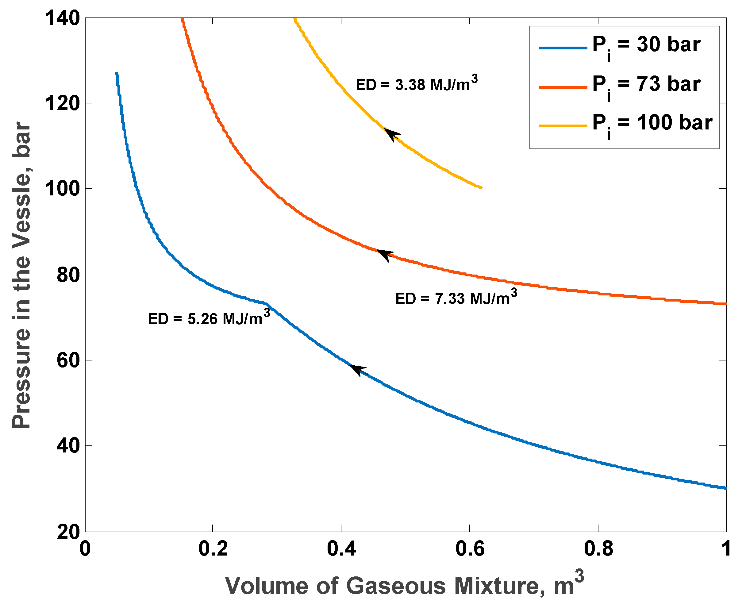
Figure 9 shows the P–V diagram for the optimal initial total CO₂ mole fraction of 88% and three different initial pressures: 30 bar (the lowest bound), 73 bar (optimal), and 100 bar (upper bound). With an initial pressure of 30 bar, the process starts from the maximal volume and ends at the minimal allowable volume, but the pressure increases to only 128 bar (approximately). With an initial pressure of 100 bar, the process starts at approximately 65% of the maximal volume. The pressure rises quickly to the maximal allowable pressure at gas volume of approximately 28% of the total volume of the vessel. With the optimal initial pressure, the process starts at the maximal volume and reaches the maximal allowable pressure at gas volume of approximately 18% of the total vessel volume.

The maximum theoretical ED attained was 7.3285 MJ/m³. Within the same pressure bounds, the theoretical ED with pure N₂ is 4.6739 MJ/m³, approximately 36% less than the optimal theoretical ED. The maximum ED with pure N₂ is 5.0949 MJ/m³, 30% less than the optimal theoretical ED, and it is obtained at initial pressure of 53 bar.

6. Conclusions and Future Work

GLIDES is a promising energy storage technology that is amenable to crowded urban areas. Its scalability makes it suitable for a wide range of storage scales, from kWh to MWh, both behind and in-front of the meter. It is simple and requires no special training nor certifications to operate and maintain. The composition of the gas in compressed air storage is a key parameter in maximizing the energy density. A second key aspect is that one of the gaseous components should be condensable at some stage in the compression process.

To increase the energy density of GLIDES, air is substituted with a mixture of carbon dioxide and nitrogen. The phase change that the carbon dioxide undergoes contributes to the increase of energy density by allowing the utilization of more volume of the vessel to store energy while maintaining the maximum pressure below the maximum allowable limit. The nitrogen, being non-condensable under room temperature, contributes to increasing the energy density by increasing the total pressure inside the storage vessel above the saturation pressure of carbon dioxide, thereby enabling greater utilization of the vessel’s volume for energy storage. A model, based on the Redlich–Kwong equation of state, was presented to solve for the pressure and volume of the gas and to calculate the energy density for any combination of initial total pressure and initial total mole fraction of carbon dioxide. Maximum energy density was attained when the system is charged with a mixture of 88% carbon dioxide and 12% nitrogen by volume to an initial pressure of 73 bar. The maximum energy density attained was 7.3285 MJ/m³, 56.8% higher than the energy density of the system using only pure nitrogen. We conclude by making evident that the use of condensable gases is a valid method for significant improvement in energy storage density using moderate pressures. For future work, a search campaign will be conducted to identify a condensable/non-condensable pair that results in even higher energy density.