Article

Thermal Modelling of a Prismatic Lithium-Ion Cell in a Battery Electric Vehicle Environment: Influences of the Experimental Validation Setup †

Technische Hochschule Ingolstadt, Institute of Innovative Mobility, Esplanade 10, 85049 Ingolstadt, Germany
*
Author to whom correspondence should be addressed.
This paper is an extended version of our paper pressed in 2019 IEEE 25th International Workshop on Thermal Investigation of ICs and Systems (THERMINIC 2019), Lecco, Italy, 25–27 September 2019.
Energies 2020, 13(1), 62; https://doi.org/10.3390/en13010062
Submission received: 18 November 2019 / Revised: 13 December 2019 / Accepted: 18 December 2019 / Published: 20 December 2019
(This article belongs to the Special Issue Thermal and Electro-thermal System Simulation 2020)

Abstract

:
In electric vehicles with lithium-ion battery systems, the temperature of the battery cells has a great impact on performance, safety, and lifetime. Therefore, developing thermal models of lithium-ion batteries to predict and investigate the temperature development and its impact is crucial. Commonly, models are validated with experimental data to ensure correct model behaviour. However, influences of experimental setups or comprehensive validation concepts are often not considered, especially for the use case of prismatic cells in a battery electric vehicle. In this work, a 3D electro–thermal model is developed and experimentally validated to predict the cell’s temperature behaviour for a single prismatic cell under battery electric vehicle (BEV) boundary conditions. One focus is on the development of a single cell’s experimental setup and the investigation of the commonly neglected influences of an experimental setup on the cell’s thermal behaviour. Furthermore, a detailed validation is performed for the laboratory BEV scenario for spatially resolved temperatures and heat generation. For validation, static and dynamic loads are considered as well as the detected experimental influences. The validated model is used to predict the temperature within the cell in the BEV application for constant current and Worldwide harmonized Light vehicles Test Procedure (WLTP) load profile.

1. Introduction

Realizing the vision of green mobility one major aspect is the reduction of worldwide car emissions by use of battery electric vehicles (BEVs). Automotive manufactures focus on lithium-ion based battery systems due to their high specific energy, low self-discharge and long cycle-life to meet the challenges of the continuously rising environmental regulations [1,2,3]. In BEVs different lithium-ion cell formats like pouch, cylindrical, and prismatic cells are used. Thereby, the thermal management is performed with various cooling concepts based on air, liquid and other approaches [3]. Cooling selection depends e.g., on the battery concepts using module architecture, or not. However, the temperature has a significant influence on the lithium-ion battery performance, ageing and safety [2]. Therefore, investigation of the heat generation and temperature development are important to examine thermal cell behaviour with regard to boundary conditions, especially the cooling conditions.
In order to answer the scientific issue of thermal battery behaviour, researchers develop different electro-(chemical)-thermal coupled simulation models [4,5,6,7,8,9,10,11,12]. Most of them are based on the general energy balance for lithium-ion based systems [13] in its detailed or simplified form.
In lithium-ion batteries, non-linear physico–chemical processes occur on different length scales from nanometre to millimetre. To face this challenge, model-based thermal investigations of battery cells are performed and reported in the literature in two fundamentally different ways: They use independent thermal models on the one hand with defined heat generation and on the other hand models with electrical or electrochemical-thermal coupling [6,7,8,10,11,12,14].
The heat generation of the former can be empirically determined [10], or e.g., modelled by a neural network [14]. The latter approach, electrically and thermally coupled behaviour, is described in the literature with different model approaches. Researchers use either the pseudo-two-dimensional modelling approach [7,8,12] based on the work of Newman et al. [15,16], equivalent circuit models (ECM) [9], and empirical models [11]. The thermal model can i.e., be executed as a point model [6] or can also be resolved three-dimensionally [7].
As in our previous research [17], in this work, an electrical ECM model with coupled 3D thermal model is used, because this approach represents a sufficient accuracy for thermal questions with at the same time acceptable computing time. The model uses the framework of the MSMD battery model architecture. This adopted general multi-scale multi-dimensional (MSMD) approach is described and used in [18,19].
In general, for validating and calibrating the model, the simulation results are compared to experimental data. Thereby, non-precise known model parameter is adjusted, i.e., optimized, to ensure correct model prediction over a defined range of model conditions. Often, important influence of the experimental setup is neither mentioned nor included in the boundary conditions within the model for validation. Especially convection conditions are often assumed to be constant [12] while validating the model’s behaviour. This generates uncertainties in the predicted thermal behaviour of the battery cell after validation. Only few studies consider this issue [4,5,20] by special setup or boundary conditions in simulation. Erhard develops an experimental setup with a pouch cell in a wind tunnel to obtain knowledge of the convection coefficient for meaningful thermal validation [4]. Furthermore, several experimental influences are monitored during the experiment used as an input to the model for validation. Rieger et al. [20] use a boundary condition for a heat flux at the terminal connection of pouch cells in the experiment. Samad et al. [5] investigate forced and natural convection conditions with prismatic cells and find uneven convection conditions depending on the position of the cell in the temperature chamber.
In this work, we focus on the automotive use case of prismatic cells in module architecture on a cooling plate-like in [6,7]. Lundgren et al. [7] suggest a detailed 3D electrochemical-thermal model with experimental validation of a prismatic cell. However, they do not consider the influences of the experiment such as wiring to the battery cycling machine or the cell’s environment. Damay et al. [6] introduce an electrical model coupled with a lumped thermal model for investigation of the thermal behaviour. Experimental influences such as insulation plates are taken into account but the constant convection condition based on literature results in uncertainty for model validation.
However, none of these studies for prismatic automotive cells take special care of experimental influences and high-resolution validation. Experimental investigations show equal temperature gradients of large-format cells [21,22] and, therefore, the necessity of spatially resolved temperature measurement and validation. Panchal et al. [21] show a temperature gradient on the casing of up to 4 K at the end of constant current discharge with a 20 Ah cell. Christen et al. [22] reveal a temperature gradient of 6.5 K at the casing of their 60 Ah prismatic cell after constant current cycling with cooling at the cell’s bottom at a temperature of 25 C . As a result of temperature gradients on the casing, neither a single temperature sensor in experiment nor an average temperature value for validation is conclusive enough. Temperature gradients occur due to cooling conditions and thermal resistances in- and outside the cell and need to be validated. Therefore, a validation concept is needed containing the differences of the experimental conditions and the use case of a prismatic cell in a BEV application.
The goal of this work is to investigate the commonly neglected influences of experimental validation setups in detail. Based on the gained knowledge a detailed validation for a 3D electro–thermal model of a prismatic lithium-ion cell is performed and the thermal behaviour in a BEV application is predicted. Therefore firstly, the focus is on the development of a single cell experimental setup for investigation of external influences. Secondly, the impact of boundary conditions on the behaviour of the used electro-thermal model is investigated. Based on this, a validation of spatially resolved temperatures and heat generation is performed for static as well as dynamic cases. Finally, the model is used to illustrate the thermal behaviour of the cell under real BEV application.

2. Modelling

2.1. General Approach

The studied cell in this work is a prismatic automotive cell. Geometric dimensions and electrical and thermal behaviour are determined experimentally and subsequently used for the parametrization of the model. Furthermore, physical properties are taken from [7,23]. Important for the thermal behaviour of the cell are the conditions of use, especially the cooling conditions. The general set up of a prismatic cell positioned in a real BEV battery module is shown in Figure 1a. In automotive application, prismatic cells are commonly stacked in modules and connected by busbars. This stack of cells is compressed for better performance. Cooling is realized by a fluid cooling system at the bottom of the cells [6]. The cooling system is commonly working with constant cooling capacity in various stages to keep the cells in the best case at constant temperature in the desired range. Simulating one cell in the middle of a module, the resulting boundary conditions of the outer walls are adiabatic beside the bottom wall where the cooling system is connected. The cell’s floor is modelled as constant temperature boundary condition, neglecting the small temperature gradient in the fluid of the cooling system for one cell to avoid detailed computational fluid dynamics simulation (CFD) of the complex cooling system in a BEV.
It is obvious that the cell in any experimental setup is experiencing slightly different boundary conditions in comparison to the model setup for simulation. Validation of a single cell in a full battery module is often not practical. Therefore, for validation of single-cell models, a more realistic validation setup is necessary that takes account for the targeted stimulation conditions as well as the application influences. The schematic of the resulting laboratory setup on single-cell level is depicted in Figure 1b. The resulting boundary conditions for model validation are comparable with Figure 1a with regard to adiabatic conditions on the models outer surfaces and constant temperature cooling conditions at the cell floor. Additionally, the bracing components, as well as the heat removal by the wiring, are considered. The modelling approach and boundary condition details are discussed in the following Section 2.2 and Section 2.3, while the experimental setup is explained in detail in Section 3.

2.2. Electro-Thermal Co-Simulation

In this work, a multi-scale multi-dimensional (MSMD) approach was adopted and used, which is described in [18,19]. It is built in ANSYS CFD as MSMD battery model [24]. The model uses the framework of the MSMD Battery Model architecture and is parametrized for an electrical ECM and 3D thermal model.
The MSMD-approach makes it possible to resolve different phenomena on different length scales. It is not feasible to solve the cell on the smallest length scale in the nanometre range in FEM analysis without generating considerable computing times and networking problems. With MSMD approach individual phenomena with sub-models are solved without resolving the entire cell in detail. Nevertheless, it is possible to obtain information on cell level with a model less detailed. The MSMD approach does neither specify the type of sub-models nor their number but defines the information exchange between the model levels [18]. The main differential equations at cell level taken from [19,24] are
ρ · C p · T t [ k · T ] = q ˙ E C h + q ˙ O h m
[ σ + · ϕ + ] = j E C h
[ σ · ϕ ] = j E C h
where (1) represents the spatial energy balance in the active material called jelly roll, the heart of a lithium-ion cell, where the electrochemic reactions and the heat generation take place. The internal energy is calculated by jelly roll’s density ρ , specific heat capacity C p , and Temperature T. The spatial heat conduction is expressed with heat transfer coefficient k. q ˙ O h m is the heat generation from ohmic losses of the current collector foils of copper/aluminium in the jelly roll [24]. q ˙ E C h is the reaction heat from the electrochemical processes taking place such as charge transfer over-potentials at the interface, and mass transfer limitations [2] (see Equation (5) for details). Equations (2) and (3) are potential equations that describe the electrical behaviour. In these equations ϕ is the phase potential, j E C h the volumetric current transfer rate, and σ the electrical conductivity of the materials [19,24].
Using an ECM for the electrical modelling of the cell’s behaviour, the voltage is represented by
U ( t ) = U O C V ( S O C , T ) U s e r i a l ( S O C , T ) U R C ( S O C , T )
whereat the voltage U is calculated in the ECM sub-model by the open circuit voltage U O C V and the voltage drop at the serial resistance U s e r i a l and the RC-element U R C . All used parameters depend on local temperature and state of charge (SOC) in the jelly roll.
The model structure of this work, implemented in the MSMD framework, is shown in Figure 2. In every time step, the model is iteratively solved for all components. The spatial temperature distribution is determined in the 3D thermal model. In every finite volume of the jelly roll, an electrical model is calculated containing the time- and local-depending temperature. Every single electrical model is implemented as an ECM. In the present model, the aim of the electro-thermal coupling is not to resolve the detailed chemical processes, but to map the resulting heat generation accurately for the thermal model. If a spatial resolution of the heat generation has aspired, ECM models represent a sufficient accuracy for thermal questions with at the same time acceptable computing time. The developed model structure is designed for first or second-order ECM. The necessary parameter sets for resistors and capacitors are determined from the current-voltage behaviour on discrete points in hybrid power pulse characterization (HPPC) test. During the simulation, these discrete data points are interpolated in the model. Additionally, the open-circuit voltage (OCV) of the used cell is determined experimentally.
The present model uses the information for resistances and capacities as a function of temperature and SOC, but is designed for n-dimensional dependencies, i.e., if a relevant dependency of the parameters on other influencing variables, such as current or ageing, becomes apparent, corresponding parameter sets can be included in the model.
With available information of local voltage drop and current load, the power dissipation in the active material of the present model is determined locally by the approach suggested by Bernardi et al. with the following equation [19,24]:
q ˙ E C h = j · [ U U O C V ( S O C , T ) ] + j · T · d U O C V d T ( S O C ) .
The first term considers the power loss due to the voltage drop at the internal resistance of the cell. The voltage U below is calculated in the ECM sub-model, the open-circuit voltage U O C V is part of the parameter set and the local current j results from the solution of the potential equations. This first part of the overall heat generation is irreversible. The second term considers the reversible heat generation based on an entropy change of the chemical system. The entropy change is shown e.g., in the temperature dependence of the OCV. In the literature, entropy change is determined experimentally for different combinations of anode/cathode pairs and recorded in the entropic heat coefficient d U / d T . This represents the reversible heat generation when multiplied with the local temperature T and the current j. The data set for the used NMC/Graphite chemistry is taken from [25].
Finally, the local heat generation is transferred in the 3D thermal model. The heat source changes temperatures, and therefore electrical resistances and heat generation, for the calculation of the next time step.

2.3. Thermal Modelling

Significant factors influencing the thermal model are the cell geometry, the associated material parameters, and the thermal boundary conditions. Geometrically, the thermal model of the prismatic cell is based on the information from the measured sectional models and a performed computer tomography and post-mortem analysis. This information is converted into a 3D CAD model, which is shown in Figure 3a. In the centre of the cell, the active material in the form of a jelly roll is modelled as one solid part with anisotropic properties of the thermal conductivity [7,23]. The copper and aluminium sheets characterize the high in-plane conductivity, while the separator in-between anode/cathode defines the lower through-plane conductivity. Furthermore, the real jelly roll is wounded. This is taken into account by a coordinate transformation regarding the conductivities in the outer rounding of the jelly roll geometry. The jelly roll’s dimensions as a result of CT analysis are shown in Figure 3b. All components are modelled as solids without considering the fluids, e.g., the electrolyte at the cell’s bottom or the air at the cell’s top. The electrolyte is simplified and modelled as solid with heat conduction. Heat transfer by convection and radiation in the top part of the cell is negligible due to small temperature differences and small areas. Additionally, the following simplifications are made creating the geometry:
  • Radii and chamfers of the cell components are neglected,
  • Thin components are considered using thin wall modelling (e.g., insulation) [24],
  • Jelly roll is modelled as a volume body with anisotropic thermal properties [7,23]
  • Junction of jelly roll sheets and current collector is modelled as a volume body.
The materials and their associated physical parameters are listed in Table 1. The jelly roll with its individual components has already been combined into one material as mentioned above.
The general targeted thermal boundary conditions were previously shown in Figure 1a. These assumptions result in a model containing only the cell geometry including full adiabatic model boundary conditions on the outer surfaces, except for the constant temperature boundary condition at the bottom. Thereby, the heat exchange by the small side surfaces and the top of the cell is neglected due to small areas and temperature differences resulting in negligible impact. Nevertheless, for a correct model validation, the conditions of the experimental setup (see Figure 1b) must be mapped as thermal boundary conditions in the simulation model. The following thermal boundary conditions are implemented in the simulation model and investigated in the results section:
  • Aluminium bracing plates and polyoxymethylene (POM) measurement plates are considered as solid bodies,
  • Adiabatic conditions are modelled on all unattached surfaces of cell and bracing plates except terminals and cell bottom,
  • Heat flow from/to the battery testers is considered at the terminal surfaces,
  • Thermal pad is included in-between constant temperature cooling plate and cell floor.
The full adiabatic model boundary conditions on the outer surfaces result from the polystyrene insulation in the experiment. Only the heat sink is the constant temperature boundary condition at the bottom. The heat flow into the battery tester is determined in the experiment using two temperature sensors on the busbars. With knowledge of geometrical parameters and physical properties, the heat flux is calculated and considered as a time-dependent boundary condition in the simulation. The removed heat is monitored in every experiment as it depends on the temperature of the connected battery tester and can, therefore, have different impact for similar experiments.
In addition to the external boundary conditions, commonly neglected modelling parameters are considered within the model of the prismatic cell. Important for proper model behaviour are e.g., heat generation in the current collectors and electrolyte at the cell bottom. If the cell’s heating is only located in the jelly roll, the local heat generation in the current collectors is missing. With increasing current collector length as in the case of the used prismatic cell, the simulation results show increasing temperature differences between model and experiment, especially at the terminals. The heat generation in the jelly roll takes place as source term in the elements of the jelly roll geometry and is calculated based on the electro-thermal coupling.
Computer tomographic analysis of the cell showed rest-electrolyte of 10–15 mL at the cell’s bottom. In [27] electrolyte influence is neglected due to long distances for conduction and low thermal conductivity of 0.6 Wm−1 K−1 [26]. In the case of this cell, the distance between the jelly roll bottom and cell casing is small with a minimum spacing of 0.4 mm. Therefore, the rest-electrolyte creates an additional thermal path at the cell bottom from the jelly roll to the cooled cell bottom, modelled by a solid body with electrolyte properties (see Table 1).
The geometrical model of the cell with all associated boundary conditions was implemented in ANSYS Fluent 19.0. The mesh of the 3D cell model contained 138k elements. The maximal adaptive time step was set to 5 s. With changing current in the used constant current profile the time step was set back to 0.1 s starting the logarithmic rise up to 5 s. In the dynamic profile, a constant time step of 1 s was applied. The used computer was a Dell Workstation with 12x Intel(R) Xeon(R) Gold 6136 CPUs and 64 GB RAM.

3. Experimental

In this work, an automotive battery cell by SANYO PANASONIC is investigated. It is a lithium-ion cell with a nominal capacity of 25 Ah based on nickel–manganese–cobalt (NMC)/graphite chemistry. The cell has a nominal voltage of 3.7 V with upper and lower cut-off voltage of 4.1 V and 3.0 V, respectively. The goal of the experimental setup is to reproduce the mentioned real BEV conditions of a cell in Figure 1b as close as possible in a laboratory setup. Therefore, a single cell measurement setup is designed and implemented. In Figure 4, the sensor schematics (a), the setup concept (b), and the final test bench of the developed setup in the temperature chamber (c) are shown. A custom cooling plate by QuickCool with thermoelectric cooler regulation is used to guarantee constant temperature cooling condition. A proper thermal connection to the cell is achieved with a thermal pad (see properties in Table 1) and a vertical clamping by an external compression unit. Polystyrene foam is used as insulation material to receive mostly adiabatic conditions (see Figure 4c). The cell’s optimal electrical performance is ensured by horizontal bracing plates made of aluminium with a thickness of 10 mm. In-between the horizontal bracing and the cell, two measurement plates of 10 mm POM are added for thermal insulation and measurement.
Overall 22 thermocouples type T class 1 by Omega with an accuracy of ± 0.5 K are used with PicoLog TC-08 data loggers to measure the temperature in an experiment on several locations. We arranged 15 thermocouples three rows and five columns inside one measurement plate (see Figure 4a) to achieve spatially-dependent temperature distribution on the casing. Additionally, thermocouples are attached to each terminal and the cooling plate. For later investigations, average values per row are used named A-D. Two sensors on each terminal side are used to measure the temperature difference on the busbar to be able to calculate the related heat flux from the cell to the battery tester.
The entire setup is placed inside a Binder KB115 temperature chamber and the cell is connected to an Arbin battery tester (LBT 5 V/ 60 A). The temperature chamber was used to guarantee uniform start and operational conditions. Unless otherwise specified, all validation tests at laboratory BEV conditions are performed at a temperature of 30 C including two hours pre-tempering prior to each experiment.
The used load profiles are either constant current cycling profiles or a commonly used dynamic profile based on the Worldwide harmonized Light vehicles Test Procedure (WLTP). The WLTP profile is used to validate the model for dynamic loads and is representative for cases as driving in the city. In Figure 5, exemplary a 75 A constant current cycling profile and the WLTP current profile are demonstrated. In case of constant current cycling, a fully charged cell is discharged to the cut-off voltage of 3 V. After a 10 s break the cell is charged with the same current until the upper cut-off voltage of 4.1 V is reached. After a second break of 10 s, one full cycle is finished and is subsequently repeated. For the dynamic load, the WLTP is transferred into a current profile per single cell. The resulting dynamic load is a transient input for the experiment and the simulation, as well.
In addition to the developed experimental setup, experiments are performed under commonly used experimental conditions for thermal investigations of battery cells. The investigated setups, such as natural/forced convective cooling or adiabatic conditions, take place with the bracing and measurement plates. All corresponding experiments start with charging of the cell at 25 C . After the charging process, the cell is tempered in the temperature chamber at 25 C . In both cases of investigated convection conditions, the chamber’s fan is either deactivated (Natural convection) or kept active (forced convection) for the duration of the cycling. A further investigated condition is the battery cell in a fully isolated setup targeting adiabatic conditions. The related experiment in this work is performed with the cell as well as measurement and bracing plates totally isolated in a box of 5 cm styrofoam plates.

4. Results and Discussions

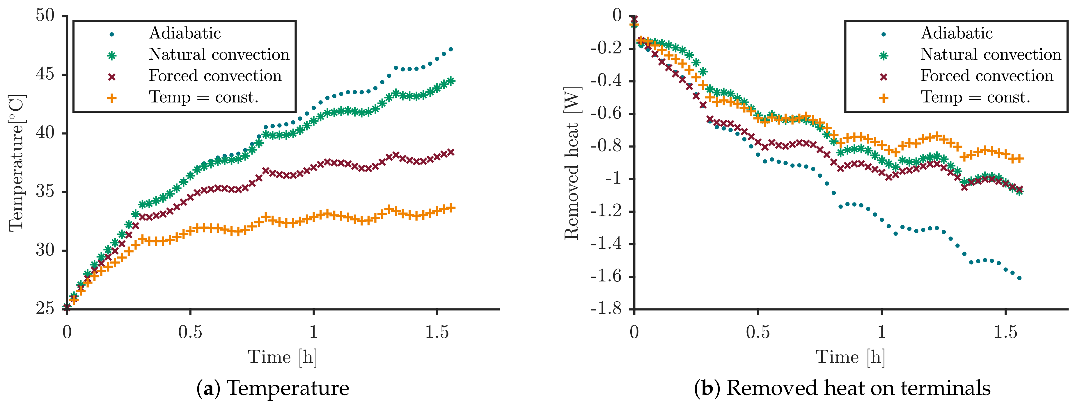
To evaluate the impact of commonly used thermal boundary conditions, the prismatic 25 Ah cell has been subjected to multiple constant current charge/discharge cycles. In Figure 6a, the general temperature behaviour of the lithium-ion cell at 25 C is shown using a cycling profile with 75 A.
In all measurements, the temperature increases with time due to heat generation during the cell’s cycling. The chronological sequence of the used current profile (see Figure 5) results in local maxima at the end of every discharge. These maxima are obtained due to the high internal heat generation at low SOC. During the first discharge, the process of heating-up is similar for all setups. However, it is apparent that the following magnitude of the temperature rise depends strongly on the boundary conditions.
In the case of natural convection the cell reaches a temperature of 45 C ( 20 K increase) at the end of the cycling. Whereas, under forced convection, the cell reaches a lower average temperature of 38 C . Samad et al. [5] show comparable results investigating a prismatic cell in an active/inactive temperature chamber. Moreover, they show a dependency on the positioning of a cell in the chamber and assume a convection coefficient that is not constant on the cell’s surface.
Thus, it is critical to use a setup like this for validation, because both, natural and forced convection, take place with unknown heat transfer conditions. Therefore, in the model validation, the associated parameters have a high uncertainty [5], are assumed as constant [12], or are commonly used as a fitting parameter. This reduces the significance of the validation and model behaviour. In [4] the issue of unknown convection coefficient is taken into account by a special experimental setup for pouch cells in a wind tunnel. In that case, the convection conditions are defined.
A solution for unknown convection is a fully isolated setup with adiabatic conditions. The fully thermally insulated cell (Adiabatic in Figure 6) shows the highest temperature increase of 22 K at the end of cycling. The main issue for validation with this setup is that targeted adiabatic conditions are not fulfilled in the experiment. In any experiment, the large wiring of the battery tester removes heat from the cell, which depends on the temperature increase in the experiment. The resulting heat removal is observable in Figure 6b. This (unwanted) heat sink removes up to 1.6 W of the heat generated in the cell during the experiment with fully insulated setup. That is up to 14% of the overall generated irreversible heat assuming an average cell resistance of 2 m Ω and 75 A cycling current. Heat removal by the wiring is an additional issue in all setups. In either case of convection compared to the full insulation setup, the overall temperature rise is lower than under adiabatic conditions. Therefore, less heat is removed by the battery tester connection. Both convection conditions lead to ~ 1 W heat removal at the end of the test, which is a significant influence. Investigating the different cell type of pouch cells in their work, Rieger et al. [20] and Erhard [4] considered heat removal on the terminals in simulation.
Avoiding uncertainties in convection conditions and monitoring heat removal by the battery tester, the laboratory single cell BEV setup in this work is developed (Temp = const. in Figure 6). With mostly adiabatic conditions and defined heat removal by conduction via the cooling plate, the uncertainties are significantly reduced in comparison to the investigated setups. The amount of (unwanted) heat removal is lower and the setup has defined cooling conditions with constant temperature cooling plate. Further benefit using the suggested setup for validation are the real use case of a battery electric vehicle. Using the laboratory BEV setup, the lowest temperatures increase of 9 K is observed. Simultaneously, 0.8 W are removed at the end of cycling, which still influences the thermal behaviour of the cell under investigation. Therefore, the heat flux at the terminals has to be monitored in every experiment because it affects the thermal behaviour significantly. It depends on the temperature of the connected battery tester and can, therefore, change for comparable experiments e.g., on different days. In the validation concept of this work, the measured heat removal is measured and used as time-dependent boundary conditions for the model validation.
In order to examine the impact of the experimental conditions of the laboratory BEV setup on the model’s behaviour, several simulations are performed respectively not considering influences from the experimental setup.
In Figure 7 the experimentally measured average terminal temperature under laboratory BEV conditions is compared to the various simulations: The boundary condition on the terminals with heat flux from/to the battery tester is neglected (No heat flux), the cell is modelled without the bracing and the measurement plates (No bracing), and the constant temperature boundary condition is directly connected to the cell bottom without interstitial material (No thermal pad).
In all simulation curves, the spikes at the end of charge/discharge are due to the 10 s breaks without heat generation taking place. Due to the graphical representation of the experimental data, the spikes are not clearly visible in the black curve (Experiment], but they exist in both, experiments and simulations, for constant current cycling with 10 s break.
In the previous figure, the heat removal by the wiring in the experiment is discussed. Not considering heat removal as a transient thermal boundary conditions in the model, the temperature increases in the corresponding simulation results (No heat flux). Starting without visible differences during the initial cycles a significant temperature increase of 1–2 K mismatch is visible for the consecutive cycling. It is obvious that other experimental conditions for validation than laboratory BEV conditions would create a much higher deviation to the experiment (see Figure 6).
Neglecting the bracing components from the experimental setup (No bracing), the cell’s average temperature shows a deviation of 2 K after the first discharge. The reason is the effect of the thermal masses in the setup on the transient process of heating up. Without the bracing components, the process of heating up takes place significantly faster, especially at the beginning. After the first cycle, the temperature differences are decreasing with consecutive cycling.
The thermal resistance between the cell and the cooling condition is realized in the experiment by a thermal pad. Assuming a direct thermal connection (No thermal pad), ideal thermal transfer leads to a maximum error of 3 K lower temperature in comparison to the experimental data. Moreover, the deviation increases with cycling time. The performed tests show, that in addition to modelling, the heat flux at the terminals and the thermal masses of bracing components, the thermal contact resistance needs to be taken into account, as well.
A thermal battery model is meaningfully validated if the heat generation and the resulting transient temperature development in the experiment and simulation show good agreement. In the used validation approach, the heat sources and the transient temperature distribution influences are validated together, considering the impact of the experimental setup.
At first, the preliminary investigated experimental and model influences are considered as boundary conditions. As a next step, the validation is performed for the heat generation and for the average and spatial dependent temperatures on different locations on the cell. Finally, an estimation of the temperature inside the jelly roll is possible.
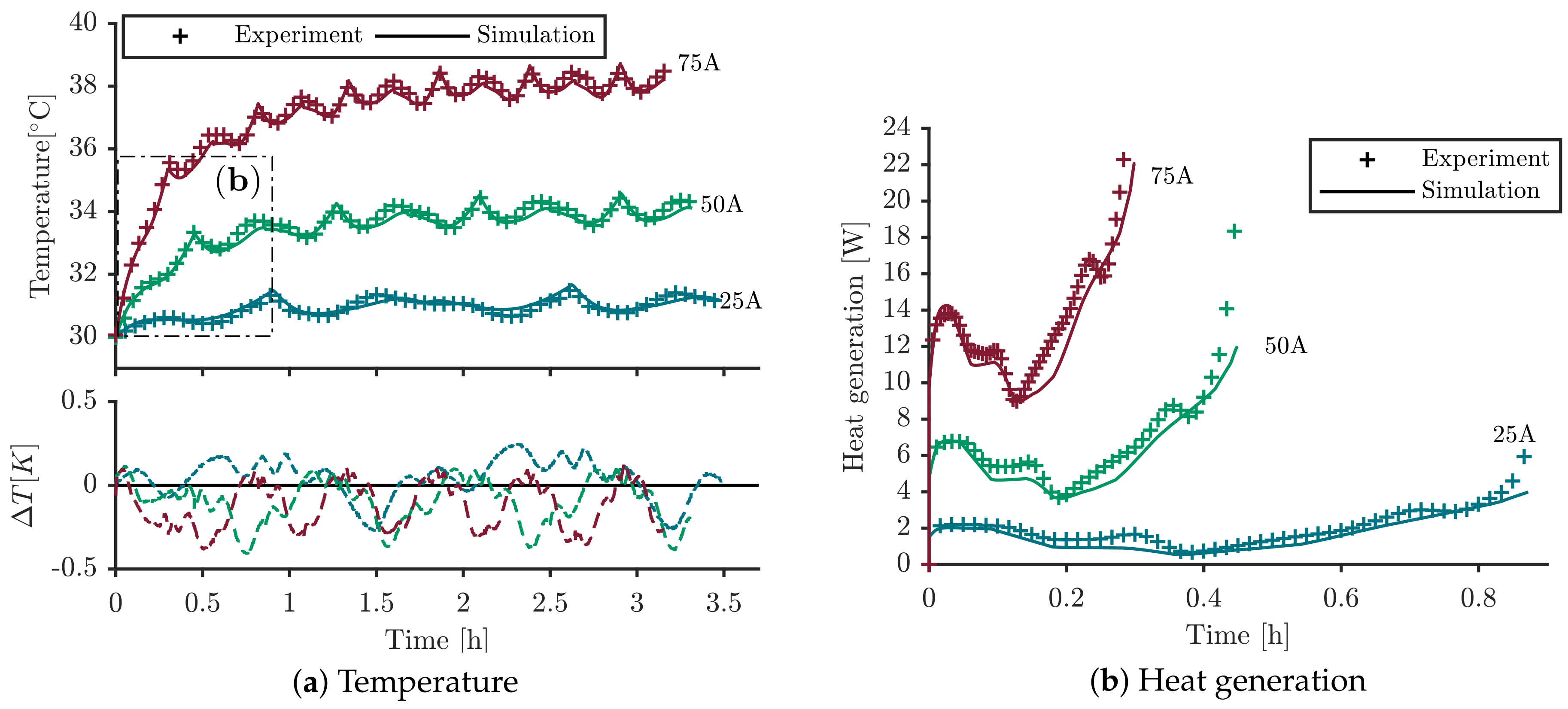
The top of Figure 8a displays the transient temperature results of the experiments and the simulations for cycling profiles with three different currents of 25 A, 50 A, and 75 A. Both experiments and simulations, show in all cases an overall increase of the temperature and a typical temperature peak at the end of charge and discharge step. This curve shape is characteristic of the used cell. At the bottom of Figure 8, the transient absolute error is shown resulting in an average root-mean-square error (RMSE) of 0.1 K for 25 A, 0.2 K for 50 A and 0.2 K for 75 A. The highest deviation for every profile exists at the end of the charge step. The error function is repetitive and does not increase with time. The errors are all below the accuracy of the used thermocouples of ± 0.5 K . Furthermore, the magnitude of the errors are in the same range and the model’s behaviour is load-independent. Thus, it can be concluded, that the model shows very good agreement with the experimental data.
To validate the heat source behaviour, the heat generation for all current profiles during the first cycle is calculated and presented in Figure 8b. The irreversible heat generation in the experiment is calculated as the measured voltage drop regarding the OCV of the cell. This calculation approach is very sensitive to the determined OCV in dependence of the SOC. Nevertheless, this approximation is sufficient to estimate the irreversible heat generation in the experiment. For the total heat generation in the experiment, the values for SOC-dependent reversible heat generation are cumulated. In the simulation, the irreversible and reversible heat generation are calculated all together by the previously mentioned co-simulation approach.
The results in Figure 8b demonstrate that the calculated heat in the simulation has the same magnitude and transient curve form as the heat generations in the experiments. The relative shape depends on the magnitude of the current. With increasing currents, the irreversible heat generation dominates the reversible term. The maximum mean error is 1 W for 75 A with a maximum deviation lower than 2 W. Especially at the end of discharge, near 10% SOC, the measured OCV differs from the real behaviour and create some uncertainty in the calculation of experimental heat generation. The average error of the heat generation in the SOC-range of 100–10% is reduced by 30% resulting in an error of 0.7 W.
The main reason for the deviations due to the fitting error, when the RC-parameters of the ECM are fitted. Furthermore, RC-parameters exist only for discrete points with a resulting interpolation error. Nevertheless, with an acceptable heat generation error in the SOC-range of 100–10%, the established model describes the thermal cell behaviour very good under laboratory single cell BEV conditions.
As already mentioned, the goal is to investigate the temperature distribution within the cell during operation with high significance using the validated model. Therefore, the accuracy of local temperature prediction is validated in addition to the average temperature by the example of 75 A current profile. In Figure 9, the temperature distribution on the casing are shown for discrete points during the constant current profile. The geometries display the simulation results including the experimental results on discrete sensor positions (x) and the related deviation of experiment and simulation in percentages.
For discrete sensor values, the model’s temperature prediction is in very good agreement. The highest measured deviation of 2.1% (±1.4% due to thermocouple accuracy) is localized at the bottom edges of the cell. As mentioned above, the thermal resistance between the cell bottom and the cooling has a great impact on simulative results. The underlying material parameters are affected by the outer clamping mechanism. This influences the results as it changes the thermal resistance of the used thermal pad. However, the overall deviation is rather small and the model reveals a good prediction of the local temperatures.
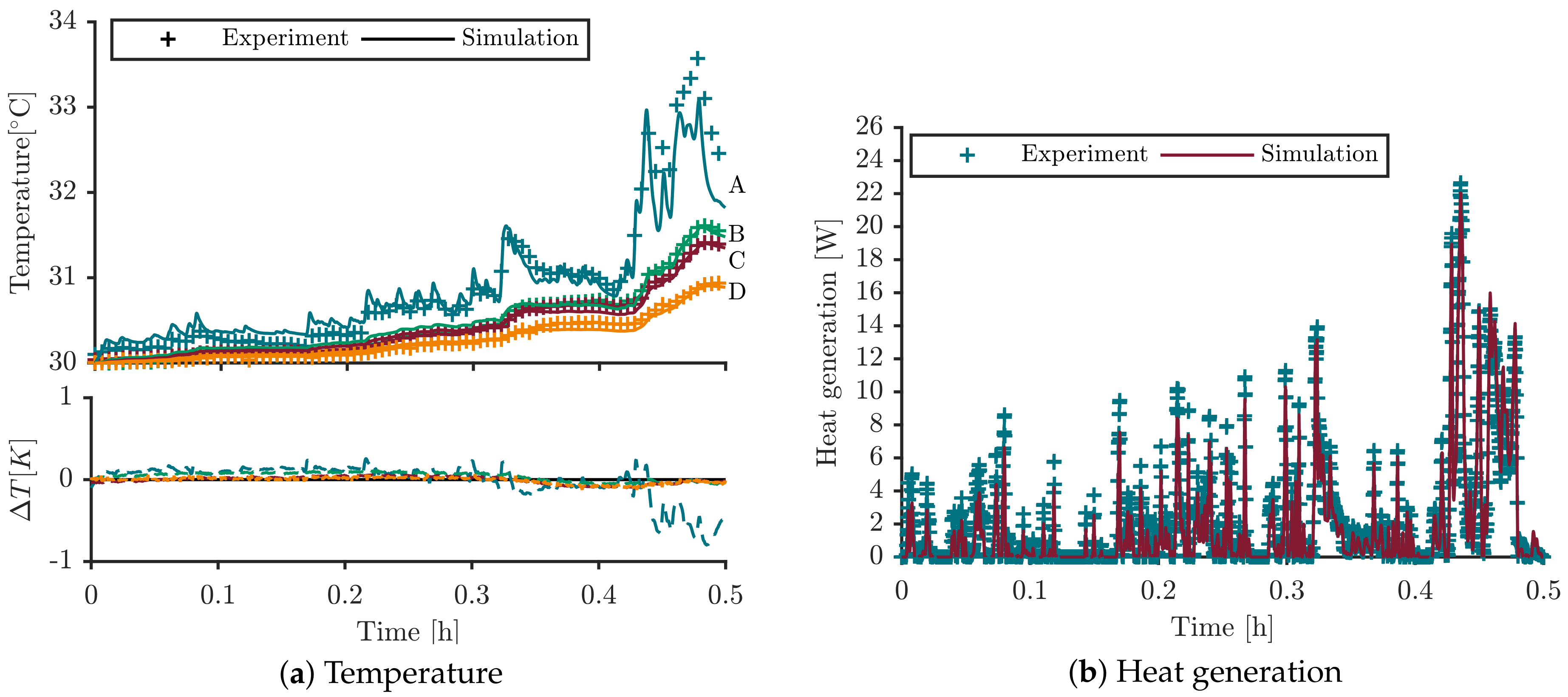
In order to investigate the thermal behaviour under dynamic operational conditions, the model is finally validated for the widely used vehicle driving profile WLTP. Starting at 95% SOC and 30 C , the 1800 s WLTP profile is operated. The results for the spatial dependence of the temperature (see nomenclature in Figure 4) and the overall heat generation are presented in Figure 10.
The simulative results in Figure 10a reproduce the temperature increase of the cell through the different sections of the WLTP (low–extra high). Very good agreement between simulation and experiment exists for the cell casing in B-D with an average RMSE values < 0.1 K. The influence of liquid cooling at the bottom in BEV concepts is visible by the increasing temperature from the cell bottom (D) to the cell top (B).
The average terminal temperature (A) shows the most dynamic behaviour with a temperature increase >10% at the end of the final section in the WLTP profile. Furthermore, the largest deviation of 0.8 K is apparent at the end. Nevertheless, the observed deviation is small with an average RMSE of < 0.3 K for section A. In general, the model describes the transient thermal cell behaviour very well under defined boundary conditions.
The comparison of related heat generation in Figure 10b shows increasing heat generation peaks with the charge throughput in the WLTP profile. At the end of the WLTP profile, the maximum peak heat generation is > 20 W. With an average error of 0.3 W the model shows good prediction of the heat generation in WLTP use case. As earlier mentioned, the estimated experimental heat generation is strongly dependent on the measured OCV. A displacement of the OCV curve of 1% SOC results in increasing error of 0.2 W. However, for a validation of the magnitude and curve form of the heat generation that is certainly a sufficient accuracy.
In comparison to constant current cycling, the thermal strain is much lower in WLTP because of large periods with little or no current. Therefore, in the case of WLTP load, no additional knowledge is achieved compared to constant current cycling in Figure 9.
In order to investigate the thermal behaviour in a real BEV scenario after successful validation, the used boundary conditions from experiment and validation are transferred to the boundary conditions of the real BEV application (see schematics in Figure 1). To verify sufficient validation conditions, the varying boundary conditions are compared in Figure 11. Thereby, the transient temperature developments for the outer (a) and inner (b) cell temperatures are shown. For the laboratory single cell setup, the overall temperature on the terminals is lower and the process of heating up is different compared to the real BEV conditions (a). The reasons are the earlier mentioned influences by the experimental setup. Nevertheless, the maximum temperature increase on the casing and on the terminals is only 2 K and 3 K in comparison to real BEV conditions in the first cycle. Subsequently, the difference between the average temperatures decreases with cycling duration reaching a minimum of 1 K respectively 2 K at the end of the test.
Most crucial temperature concerning safety, ageing, and cooling issues is the jelly roll temperature. In Figure 11b the estimated maximum and average jelly roll temperatures are given. There is a temperature increase for real BEV conditions of 1–2 K but the increase is similar for mean and maximum temperature. Overall, the used laboratory BEV setup reproduces the real BEV application very well and transfers the boundary conditions of a battery system to a practical single-cell setup.
Evaluating the effects of the boundary conditions in real BEV environment, the local temperature peaks at the end of discharge are more pronounced inside the jelly roll than on the surface. Moreover, the terminal temperature in case of real BEV conditions shows a similar transient behaviour compared to the mean jelly roll temperature. Therefore, the jelly roll temperature can be approximated by measuring the terminal temperature in real BEV application. This is important e.g., for proper thermal management systems.
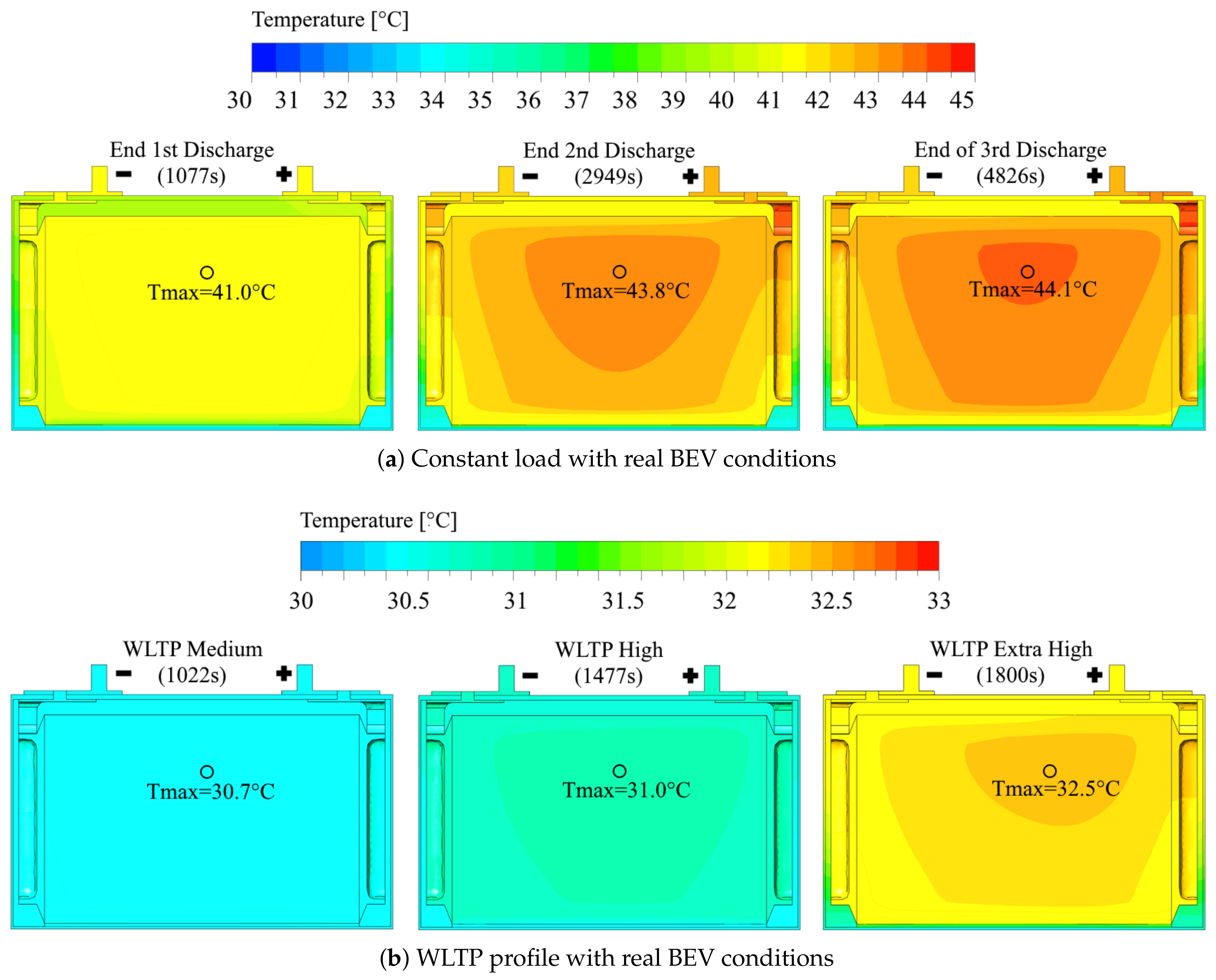
The results for the temperature distribution on the central symmetry plane inside the cell are displayed in Figure 12. The stated value in each sub-figure (◯) is the maximum jelly roll temperature calculated in simulation under real BEV conditions. The heat generation of the cell with constant current cycling (Figure 12a) leads to a maximum temperature inside the jelly roll up to 44.1 C at the end of the third discharge. The highest temperature is reached in the upper part of the jelly roll. The reason for the vertical location is the heat generation inside the jelly roll in combination with the cooling system located at the bottom. Additionally, the increase of the vertical temperature gradient with time is revealed on the casing. The gradient increases from 5 K after the first discharge up to 8 K after the third discharge. Whereas the vertical position is affected by the cooling conditions, the horizontal position is slightly located towards the cathode current collector due to different material properties on anode and cathode. This results in different temperatures in the current collectors. Similar temperatures compared to the jelly roll are detected in the positive current collector due to the ohmic heat generation at the location of high current density.
Investigating the cell’s temperature behaviour in the WLTP, the low thermal stress created by the load is revealed in Figure 12b. Especially in the first sections of the WLTP, the average heat load and the resulting temperature increase is small. Thus, a good regulation of the cell’s temperature by the defined coolant temperature is possible. In the final section of the WLTP, the temperature inside the jelly roll increases up to 32.5 C . In general, during the WLTP, the same temperature distribution results inside the jelly roll compared to constant current load but with much lower overall temperature. During periods of high loads towards the end of the profile at 1800 s, the terminal temperature increases much faster due to the direct connection to the heat generation within the current collectors.
The temperature behaviour with real BEV conditions is much more important to investigate under load conditions with high thermal impact than under conditions with low thermal impact. The temperature development in dynamic WLTP profile reveals that such cases are not challenging with the studied prismatic cells in BEV cooling conditions. High current loads in reality such as fast charging or continuous high velocity of vehicles are much more challenging for performance, safety and lifetime issues. With the developed and validated 3D electro–thermal model, further investigation in the field of cooling approaches and module influences are possible.

5. Conclusions

In this work, an experimental setup was developed that transfers the boundary conditions of a real BEV battery system with module architecture to a laboratory single cell setup. The setup is used for validation of a 3D thermal model of a prismatic 25 Ah lithium-ion battery cell. The influences of different commonly used experimental setups for thermal battery model validation are investigated and compared to the designed setup. The results show, that not only the general ambient conditions but also additional effects, such as the battery tester connection, have a strong impact on the measured cell temperature. In targeted adiabatic conditions over 14% of the produced heat are removed through the wiring. Therefore, the removed heat has to be monitored in the experiment and used as a transient boundary condition for validation. Further influences, such as thermal masses of the bracing component in the experiment are shown to be important for accurate model behaviour.
To guarantee the model’s significance, a detailed validation approach was performed. The previously determined experimental and modelling influences on the thermal cell behaviour were considered as boundary conditions in the validation model. Subsequently, the model’s thermal behaviour was validated for static loads as well as for dynamic profiles. The obtained simulation results are in very good agreement with the experimental data collected at various profiles. For proper validation, not only the average temperature but also local temperatures on discrete sensor positions are validated. The model reveals maximum local errors of ~2% at high current cycling. The maximum average RMSE value for dynamic as well as static profiles is < 0.4 K and therefore under the accuracy of the used thermocouples of ± 0.5 K . After successful validation, the model is used to predict the temperature in a real BEV application. First, the differences between laboratory setup and real application are evaluated by simulation. The evaluation indicates that the developed setup reproduces the real BEV conditions adequately. Considering real BEV conditions with fully validated model, the simulations reveal small thermal effects in the cell during the WLTP profile. During constant current profiles, exemplary for fast charging, the cell experiences stronger thermal effects with increasing temperature in the jelly roll up to 44.1 C and gradients between anode/cathode, as well as in vertical direction towards the cooling system.
Further work with the validated model will focus on the effects of cooling conditions in BEVs and the module’s specific conditions and their influence on the cell’s thermal behaviour such as additional power loss by electronic components.

Author Contributions

Conceptualization, C.E., G.E. and J.K.; methodology, J.K. and L.K.; software, J.K.; validation, J.K. and L.K.; investigation, J.K., L.K. and G.E.; writing—original draft preparation, J.K.; writing—review and editing, C.E., G.E., L.K. and J.K.; visualization, J.K.; supervision, G.E. and C.E.; project administration, C.E. All authors have read and agreed to the published version of the manuscript.

Funding

This work was funded by the AUDI AG within the scope of an ongoing research project.

Acknowledgments

The authors wish to acknowledge M. Keppeler (ZSW) for the CT-Analysis and D. Schneider (Technische Hochschule Ingolstadt), M. Hinterberger (Audi AG), B. Rieger (Audi AG) and R. Reinelt (ANSYS Germany) for the extensive discussions.

Conflicts of Interest

The authors declare no conflict of interest.

Abbreviations

The following abbreviations are used in this manuscript:
BEVBattery electric vehicle
ECMEquivalent circuit model
MSMDMulti-scale multi-dimensional
NMCNickel–manganese–cobalt
OCVOpen circuit voltage
RSMERoot mean square error
SOCState of charge
TECThermoelectric cooler
WLTPWorldwide harmonized Light vehicles Test Procedure

References

  1. Rao, Z.; Wang, S. A review of power battery thermal energy management. Renew. Sustain. Energy Rev. 2011, 15, 4554–4571. [Google Scholar] [CrossRef]
  2. Bandhauer, T.M.; Garimella, S.; Fuller, T.F. A Critical Review of Thermal Issues in Lithium-Ion Batteries. J. Electrochem. Soc. 2011, 158, R1. [Google Scholar] [CrossRef]
  3. Wang, Q.; Jiang, B.; Li, B.; Yan, Y. A critical review of thermal management models and solutions of lithium-ion batteries for the development of pure electric vehicles. Renew. Sustain. Energy Rev. 2016, 64, 106–128. [Google Scholar] [CrossRef]
  4. Erhard, S. Multi-Dimensional Electrochemical-Thermal Modeling of Lithium-Ion Batteries. Ph.D. Thesis, Institute EES, Technical University Munich, Munich, Germany, 2017. Available online: http://mediatum.ub.tum.de/doc/1338266/1338266.pdf.
  5. Samad, N.A.; Siegel, J.B.; Stefanopoulou, A.G. Parameterization and Validation of a Distributed Coupled Electro-Thermal Model for Prismatic Cells. In ASME 2014 Dynamic Systems and Control Conference; American Society of Mechanical Engineers: New York, NY, USA, 2014; p. V002T23A006. [Google Scholar] [CrossRef] [Green Version]
  6. Damay, N.; Forgez, C.; Bichat, M.P.; Friedrich, G. Thermal modeling of large prismatic LiFePO4/graphite battery. Coupled thermal and heat generation models for characterization and simulation. J. Power Sources 2015, 283, 37–45. [Google Scholar] [CrossRef]
  7. Lundgren, H.; Svens, P.; Ekström, H.; Tengstedt, C.; Lindström, J.; Behm, M.; Lindbergh, G. Thermal Management of Large-Format Prismatic Lithium-Ion Battery in PHEV Application. J. Electrochem. Soc. 2016, 163, A309–A317. [Google Scholar] [CrossRef]
  8. Tourani, A.; White, P.; Ivey, P. A multi scale multi-dimensional thermo electrochemical modelling of high capacity lithium-ion cells. J. Power Sources 2014, 255, 360–367. [Google Scholar] [CrossRef]
  9. Giegerich, M.; Koffel, S.; Filimon, R.; Grosch, J.L.; Fuhner, T.; Wenger, M.M.; Gepp, M.; Lorentz, V. Electrothermal modeling and characterization of high capacity lithium-ion battery systems for mobile and stationary applications. In Proceedings of the IECON 2013, Vienna, Austria, 10–13 November 2013; IEEE: Piscataway, NJ, USA, 2013; pp. 6721–6727. [Google Scholar]
  10. Forgez, C.; Vinh Do, D.; Friedrich, G.; Morcrette, M.; Delacourt, C. Thermal modeling of a cylindrical LiFePO4/graphite lithium-ion battery. J. Power Sources 2010, 195, 2961–2968. [Google Scholar] [CrossRef]
  11. Yi, J.; Kim, U.S.; Shin, C.B.; Han, T.; Park, S. Three-Dimensional Thermal Modeling of a Lithium-Ion Battery Considering the Combined Effects of the Electrical and Thermal Contact Resistances between Current Collecting Tab and Lead Wire. J. Electrochem. Soc. 2013, 160, A437–A443. [Google Scholar] [CrossRef]
  12. Ye, Y.; Shia, Y.; Cai, N.; Lee, J.; He, X. Electro-thermal modeling and experimental validation for lithium ion battery. J. Power Sources 2012, 199, 227–238. [Google Scholar] [CrossRef]
  13. Bernardi, D.; Pawlikowski, E.; Newman, J. A General Energy Balance for Battery Systems. J. Electrochem. Soc. 1985, 132, 5. [Google Scholar] [CrossRef] [Green Version]
  14. Panchal, S.; Dincer, I.; Agelin-Chaab, M.; Fraser, R.; Fowler, M. Experimental and simulated temperature variations in a LiFePO4-20 Ah battery during discharge process. Appl. Energy 2016, 180, 504–515. [Google Scholar] [CrossRef]
  15. Doyle, M.; Fuller, T.; Newman, J. Modeling of Galvanostatic Charge and Discharge of the Lithium/Polymer/Insertion Cell. J. Electrochem. Soc. 1993, 140, 1526. [Google Scholar] [CrossRef]
  16. Fuller, T.F.; Doyle, M.; Newman, J. Simulation and Optimization of the Dual Lithium Ion Insertion Cell. J. Electrochem. Soc. 1994, 141, 1. [Google Scholar] [CrossRef] [Green Version]
  17. Kleiner, J.; Komsiyska, L.; Elger, G.; Endisch, C. Modelling of 3D Temperature Behavior of Prismatic Lithium-Ion Cell With Focus on Experimental Validation Under Battery Electric Vehicle Conditions. In Proceedings of the IEEE 25th International Workshop on Thermal Investigation of ICs and Systems (THERMINIC 2019), Lecco, Italy, 25–27 September 2019. [Google Scholar]
  18. Kim, G.H.; Smith, K.; Lee, K.J.; Santhanagopalan, S.; Pesaran, A. Multi-Domain Modeling of Lithium-Ion Batteries Encompassing Multi-Physics in Varied Length Scales. J. Electrochem. Soc. 2011, 158, A955. [Google Scholar] [CrossRef]
  19. Madani, S.S.; Swierczynski, M.J.; Kaer, S.K. The discharge behavior of lithium-ion batteries using the Dual-Potential Multi-Scale Multi-Dimensional (MSMD) Battery Model. In Proceedings of the 2017 Twelfth International Conference on Ecological Vehicles and Renewable Energies (EVER), Monte Carlo, Monaco, 11–13 April 2017; IEEE: Piscataway, NJ, USA, 2017; pp. 1–14. [Google Scholar] [CrossRef]
  20. Rieger, B.; Erhard, S.V.; Kosch, S.; Venator, M.; Rheinfeld, A.; Jossen, A. Multi-Dimensional Modeling of the Influence of Cell Design on Temperature, Displacement and Stress Inhomogeneity in Large-Format Lithium-Ion Cells. J. Electrochem. Soc. 2016, 163, A3099–A3110. [Google Scholar] [CrossRef]
  21. Panchal, S.; Dincer, I.; Agelin-Chaab, M.; Fraser, R.; Fowler, M. Experimental temperature distributions in a prismatic lithium-ion battery at varying conditions. Int. Commun. Heat Mass Transf. 2016, 71, 35–43. [Google Scholar] [CrossRef]
  22. Christen, R.; Rizzo, G.; Gadola, A.; Stöck, M. Test Method for Thermal Characterization of Li-Ion Cells and Verification of Cooling Concepts. Batteries 2017, 3, 3. [Google Scholar] [CrossRef] [Green Version]
  23. Bohn, P.; Liebig, G.; Komsiyska, L.; Wittstock, G. Temperature propagation in prismatic lithium-ion-cells after short term thermal stress. J. Electrochem. Soc. 2016, 313, 30–36. [Google Scholar] [CrossRef]
  24. ANSYS INC. ANSYS Fluent MANUAL, no. 19.0. Available online: http://www.ansyshelp.ansys.com (accessed on 5 November 2019).
  25. Schuster, E.; Ziebert, C.; Melcher, A.; Rohde, M.; Seifert, H.J. Thermal behavior and electrochemical heat generation in a commercial 40 Ah lithium ion pouch cell. J. Power Sources 2015, 286, 580–589. [Google Scholar] [CrossRef]
  26. Chen, S.C.; Wan, C.C.; Wang, Y.Y. Thermal analysis of lithium-ion batteries. J. Power Sources 2005, 140, 111–124. [Google Scholar] [CrossRef]
  27. Hopp, H. Thermal Management of High-Performance Vehicle Traction Batteries using Coupled Simulation Models; Research; Springer: Wiesbaden, Germany, 2016. [Google Scholar] [CrossRef]
Figure 1. Schematic boundary conditions for a prismatic cell in battery electric vehicle (BEV) application for simulation and experiment: (a) real BEV scenario in a module of a battery system and (b) laboratory BEV scenario with single cell experimental setup using a thermoelectric cooler (TEC).
Energies 13 00062 g001
Figure 2. Model structure for electro–thermal co-simulation of 3D thermal model, multiple electrical equivalent circuit models (ECM) models and spatial heat generation models.
Energies 13 00062 g002
Figure 3. (a) The 3D CAD geometry and outer dimensions of prismatic 25 Ah cell with jelly roll, anode/cathode current collectors, +/− terminals, and casing. (b) Computer tomography (CT) results for jelly roll dimensions.
Energies 13 00062 g003
Figure 4. Experimental setup with nomenclature and positions of temperature sensors (a), concept of experimental setup (b), and top view photograph of the cell on test bench without insulation at the top (c).
Energies 13 00062 g004
Figure 5. Constant current profile (e.g., 75 A) and dynamic current WLTP profile used for experiment and simulation.
Energies 13 00062 g005
Figure 6. Measured transient behaviour of 25 Ah cell at 75 A cycling under varying thermal boundary conditions. Staring conditions as well as cooling plate and/or temperature chamber are set to 25 C : (a) average cell temperature with time, and (b) related removed heat by the wiring on the terminals.
Energies 13 00062 g006
Figure 7. (top) Average terminal temperature for experiment and simulation at 75 A cycling of cell under laboratory BEV conditions with varying experimental influences. Staring conditions as well as cooling plate temperature are set to a temperature of 30 C . (bottom) Corresponding temperature deviation to experimental results.
Energies 13 00062 g007
Figure 8. Validation of experiment and simulation for different constant current cycling of cell under laboratory BEV conditions with: (a) overall temperature and corresponding temperature difference and (b) heat generation within the first cycle. Staring conditions as well as cooling plate temperature are set to a temperature of 30 C .
Energies 13 00062 g008
Figure 9. Temperature distribution on the casing of 25 Ah cell for discrete time steps (1077 s, 2949 s, and 4826 s) of constant current cycling with 75 A under laboratory BEV conditions. Staring conditions as well as cooling plate temperature are set to a temperature of 30 C . On discrete sensor positions (x) experimental measurement results and deviation of simulation are included.
Energies 13 00062 g009
Figure 10. Validation of experiment and simulation for dynamic WLTP cycling of cell under laboratory BEV conditions with: (a) Overall spatially-resolved temperature (nomenclature A–D as in Figure 4) and corresponding spatially-resolved temperature difference and (b) heat generation during WLTP. Staring conditions as well as cooling plate temperature are set to a temperature of at 30 C .
Energies 13 00062 g010
Figure 11. Simulation results for constant current cycling with 75 A of 25 Ah cell at 30 C under varying BEV conditions: (a) overall temperature and corresponding temperature difference of outer temperatures (nomenclature A–D in Figure 4). (b) Overall temperature and corresponding temperature difference of jelly rolls max. and mean temperatures.
Energies 13 00062 g011
Figure 12. Temperature distribution on the central symmetry plane inside the 25 Ah cell under real BEV conditions at 30 C for constant current cycling with 75 A (a) and dynamic WLTP profile (b). On discrete positions (o) the maximum jelly roll temperature in simulation is included.
Energies 13 00062 g012
Table 1. Used materials and thermal properties of 3D thermal model of prismatic 25 Ah cell.
MaterialPoint of Use ρ C p λ
[ kgm 3 ] [ Jkg 1 K 1 ] [ Wm 2 K 1 ]
Aluminium acasing, collector, terminal2700900238
Copper acollector, terminal8700385400
Insulation ball insulations147011900.18
Thermal pad cconnection cooling27409032.22
Electrolyte drest-electrolyte113020550.6
Jelly roll ajelly roll20431371in-plane 33 e
trough-plane 0.7 e
a [23], b [7], c data-sheet, d [26], e cell manufacturer.

