Abstract
Depending on its operating conditions, traditional soot blowing is activated for a fixed time. However, low-frequency soot blowing can cause heat transfer efficiency to decrease. High-frequency soot blowing not only wastes high-pressure steam, but also abrades surface pipes, reducing the working life of a heat exchange device. Therefore, it is necessary to design an online ash fouling monitoring system to perform soot blowing that is dependent on the status of ash accumulation. This study presents an online monitoring model of ash-layer thermal resistance that reflects the degree of ash fouling. A wavelet threshold denoising algorithm was applied to smooth the thermal resistance of the ash layer calculated by the heat balance mechanism model. Thus, the variation in thermal resistance becomes more visible, which is more conducive to optimizing the operation of soot blowing. The designed Support Vector Regression (SVR) model could achieve the online prediction of thermal resistance denoising for low-temperature superheaters. Experimental analysis indicates that the prediction accuracy was 98.5% during the testing phase. By using the method proposed in this study, online monitoring of heating surfaces during the ash fouling process can be realized without adding complicated and expensive equipment.
1. Introduction
In the Chinese economy, the coal-fired boiler continues to play a significant role in converting heat energy into steam or hot water [1]. The energy conservation and environmental protection policies of coal-fired boilers in China have been continuously strengthened in recent years [2]. Many cities are carrying out energy-saving and emission-reduction renovations of boilers. In 2015, China pledged to reduce its CO2 emissions per unit of GDP by 60–65% by 2030 compared with the levels in 2005 [3,4]. Therefore, China’s coal-fired boilers have rapidly developed in the direction of high parameters and large capacities in recent years [5]. Supercritical and ultra-supercritical units with rated power generations greater than 600 MW have gradually become the dominant direction of coal-fired units.
Since the end of July 2017, China has put into operation 101 units of 1000 MW ultra-supercritical units. However, with the increase of boiler capacity and parameters, especially the improvement of steam parameters, the problem of ash and slag in boiler furnaces and on convection heating surfaces has become more serious. In the furnace combustion process, ash fouling and slagging on heating surfaces has always been one of the critical factors affecting heat transfer efficiency. After the pulverized coal particles are burned, part of the fly ash passes through the platen superheater, high-temperature superheater, low-temperature superheater, reheater, economizer, air preheater and so on. Ash and slag are deposited on the heating surfaces of all levels. The slope and superheater areas are sometimes covered by massive ash deposits, which in severe cases can cause undesirable unit shutdowns [6]. Due to the small thermal conductivity of the ash, ash accumulation increases the thermal resistance of the heating surface and deteriorates the heat exchange, which in turn causes the exhaust temperature to increase and the boiler efficiency to decrease. When the ash accumulation is serious, ash blockage will occur in the flue, resulting in increased ventilation resistance and reduced boiler output. Sometimes, a power plant is even forced to shut down its furnaces. In addition, high-temperature corrosion and wear of the heating-surface metal tube (caused by ash and slagging) are main factors that can result in boiler tube explosion. Dong et al. [7] introduced a comprehensive experiment in which fly ash particles were impacted under controlled conditions against a flat steel surface to understand the ash deposition process in a pulverized coal boiler system. A systematic study was conducted at a coal-fired power plant, including detailed fuel analysis, boiler and soot-blower characteristics and optimization of slagging in the furnace [8].
The most common solution is to clean the heating surface using various types of soot blowers, as soot blowing can ensure the safety and economy of boiler operation. Shi et al. [9] firstly proposed a cleanliness factor model to monitor the ash deposition status of air preheaters. The analysis of fouling kinetics and optimization of the soot-blowing strategy are then performed to optimize steam consumption and heat transfer efficiency. Shi et al. [10] also established an optimization model of soot blowing on a boiler’s economizers. The measurement data and basic thermodynamic calculation data of the distributed control system (DCS) of a thermal power plant are used to calculate the fouling rate of the heated surface in real time. The traditional soot blowing method is purged for a fixed time, depending on operating conditions [11]. The low-frequency soot blowing process can cause heat transfer efficiency to decrease, diminishing a boiler’s performance. High-frequency soot blowing, on the other hand, can not only result in the waste of high-pressure steam, but also abrade surface pipes, causing enormous thermal stress and reducing the working life of the heat exchange device while increasing the maintenance cost of the soot blower. Therefore, regular soot blowing will not meet the economic and efficiency requirements of soot blowing.
Different methods for automatic soot blowing that are dependent on the severity of ash in the heated area have become a hot research topic. However, the fouling degree of the heating surface includes many factors, including the characteristics of nonlinearity and strong coupling. This is difficult to simulate with a precise physical model [12], so it is particularly important to establish an online monitoring model that uses thermal resistance to characterize the fouling degree of the heating surface. Through accurate online monitoring of the fouling level on a boiler’s heating surface, soot blowing optimization can be implemented to improve the economy and efficiency of boiler operation.
There are three primary methods for predicting the fouling level of a heating surface, including ash fouling monitoring based on instrumental measurements (direct method), ash fouling monitoring based on a mechanism model (indirect method) and ash fouling monitoring based on a data-driven model (indirect method).
In boiler furnaces, instrumentation-based ash fouling monitoring systems include an acoustic pyrometry system. Multi-path measurement of the temperature field in the boiler furnace is carried out by an acoustic generator and an acoustic receiver. The geometric pixel segmentation and regularization algorithm are used to reconstruct the two-dimensional temperature field [13]. Acoustic pyrometry technology is used to monitor the temperature change of flue gas on the local heating surface in the boiler furnace, and a new cleaning factor is defined to characterize the shift in the ash fouling degree [14]. However, acoustic pyrometry technology has its limitations: it can only measure the temperature change of the local heating surface; most of the heating surface is unmeasurable; and additional acoustic sensors are required.
An ash fouling monitoring system based on a mechanism model mainly uses the heat transfer principle to establish the heat transfer model of heating surfaces, and it selects the cleaning factor to reflect the fouling degree of the heating surface [15]. The boiler-side heat absorption models are established to calculate the heat absorption rate of the working fluid in the boiler, including heat exchanger, metal wall and heat loss [16]. The superheater model is used to analyze the effect of the ash layer on the outer tube surfaces and the scale-layer deposit on the inner tube surfaces [17]. Digital signal processing tools are also widely used in the data processing and analysis of boiler monitoring to optimize the ash fouling monitoring system. A dual-extended Kalman filter has been used to estimate the influencing factors of ash deposition, and a cleaning factor indicator has been applied to reflect the fouling degree of heating surfaces [18]. Sobota introduced a method for determining the heat-flow parameters of a steam boiler [19] that can perform online calculations of heating flow rates absorbed by boiler furnaces and superheaters. These parameters can determine the degree of slagging in the furnace. Monitoring the performance of a unit and determining the degree of slagging in the furnace is of great importance. Pronobis studied the influence of biomass co-combustion on the fouling of boiler convection surfaces [20], determining that the co-combustion of straw can cause severe chloride corrosion in superheater tubes. Meanwhile, adopting properly organized soot-blowing technology can eliminate the more serious problem of ash accumulation during the biomass fuel combustion process. Feng et al. [21] built a model of multi-pressure heat recovery steam generator (HRSG) based on the laws of thermodynamics and incorporated energy balance equations for heat exchangers while analyzing flue gas and water/steam parameters such as temperature, pressure, steam mass flow rate and the heat efficiency of different heat exchangers. Tong et al. [22] developed a model to solve the heat transfer calculation of multi-sectional regenerative air heaters (which usually have several layers), and they designed a computational procedure through which to carry out the model. Feng et al. [23] analyzed the steam mass flow rate and outlet temperature of HRSG based on several parameters. This analysis was based on the laws of thermodynamics, and incorporated into the energy balance equations for heat exchangers.
An ash fouling monitoring system based on a data-driven model uses machine learning algorithms to identify and map the relationships between data, avoiding the establishment of complex nonlinear coupled physical models. Enrique et al. (2005) introduced an artificial neural network (ANN) into the prediction of a fouling degree on the boiler heating surface [24]. A probabilistic prediction model for soot blowing based on an artificial neural network and an adaptive neuro-fuzzy inference system was proposed that could avoid the establishment of the nonlinear complex theoretical models involved in fouling dynamics [25]. Temperature differences between the two sides of the tube and shell and the efficiency of the heat exchanger have been predicted based on a local linear wavelet neural network model [26]. The particle swarm optimization (PSO) algorithm can be applied to the hyper-parameter optimization of the support vector machine (SVM) to establish a fouling prediction model for the heat exchanger, which provides another method for the fouling prediction of the heat exchanger [27]. However, the robustness of the pure data-driven model is weak, and easily deviates from the actual value under small disturbances.
To enhance the stability and prediction accuracy of ash fouling monitoring systems, this study proposes a method of combining the mechanism model and the data-driven model for the fouling prediction of boiler heating surfaces.
2. Online Ash Fouling Monitoring Model of a Low-Temperature Superheater
Figure 1 shows the overall framework of the training process for the ash accumulation monitoring model. Firstly, according to the principle of heat balance, a heat transfer mechanism model is established to calculate the thermal resistance of the ash layer, after which the wavelet threshold denoising algorithm is used to filter out the noise fluctuation in the thermal resistance. Finally, this paper establishes an online fouling prediction model for heating surfaces based on support vector regression (SVR) [28]. This method can filter jagged fluctuations in the thermal resistance data and predict the ash fouling severity of low-temperature superheaters online, providing more-favorable conditions for the research of further soot blowing optimization strategies.
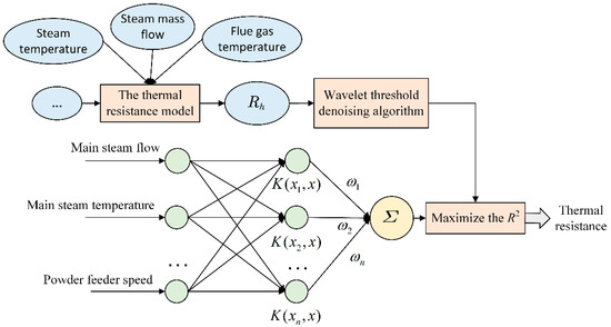
Figure 1.
The training model for the ash fouling accumulation monitoring of boiler heating surfaces.
2.1. The Thermal Resistance Model of a Low-Temperature Superheater
As shown in Figure 2, heat balance and the heat transfer calculation of heating surfaces are based on the basic theory of boiler thermal balance and performed one by one along opposite directions of the flue gas flow from the outlet of the air preheater. The inlet working-fluid temperature of the low-temperature superheater is calculated according to the heat balance principle—Equations (1) and (2) for the working fluid side and the flue gas side based on the known inlet and outlet gas temperatures of each heating surface, the working fluid outlet parameters and the pipe arrangement structure of each heating surface. Heat transfer Equation (7) can then be applied to calculate the heat transfer coefficient of the boiler’s low-temperature superheater.
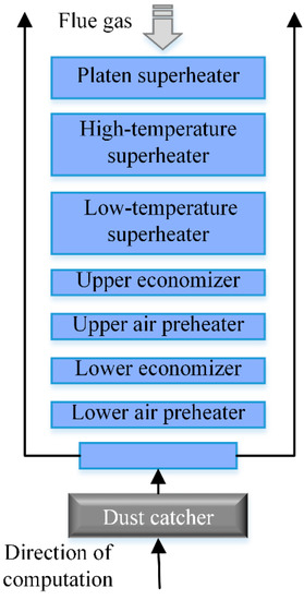
Figure 2.
The flue gas flow process on the heating surfaces of the boiler.
Heat absorption on working fluid side:
Heat release on flue gas side:
where is the convection heat absorption on the working fluid side; is the convection heat release on the flue gas side; is the quantity of the working fluid flow; denotes the calculating fuel quantity; and represent the enthalpy of the inlet working fluid and outlet working fluid, respectively; and are the enthalpy of the inlet flue gas and outlet flue gas, respectively; is the reduced value of steam enthalpy in the desuperheater; is the heat retention coefficient; is the air leakage coefficient; and is the theoretical cold air enthalpy.
Physical parameters such as , , , , , and so on are collected in the distributed control system (DCS), and , , and so on can be obtained through manual boiler design and thermal calculation. According to the heat balance equation , the enthalpy of the inlet working fluid at the low-temperature superheater is as follows:
According to the enthalpy temperature table of superheated steam, as shown in Figure 3, the corresponding inlet working fluid temperature is expressed as follows:
where is superheated steam enthalpy, and is superheated steam pressure.
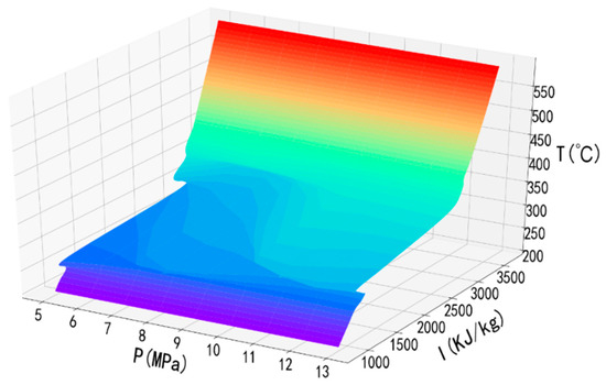
Figure 3.
The enthalpy diagram of superheated steam.
Next, the logarithmic mean temperature difference is obtained from the inlet and outlet working fluid temperatures and the inlet and outlet flue gas temperatures, which can be described as follows:
where is the difference between the inlet temperature of the flue gas side and the inlet temperature of the working fluid side of the low-temperature superheater, and is the difference between the outlet temperature of the flue gas side and the outlet temperature of the working fluid side of the low-temperature superheater.
When the maximum temperature difference and the minimum temperature difference are satisfied using , the logarithmic mean temperature difference can be simplified as follows:
Finally, the actual heat transfer coefficient of the heating surface should be
where is the heat transfer area of the low-temperature superheater.
Taking the low-temperature superheater as an example, Figure 4 depicts the heat transfer in a single superheater tube. The tubular convective heating surface is regarded as a heat transfer model of multi-layer cylindrical wall, and the heat transfer coefficient K is calculated as follows:
where is the heat release coefficient of the flue gas side; is the heat absorption coefficient for the working fluid side; is the ash-layer thermal conductivity; is the metal tube thermal conductivity; is the scale-layer thermal conductivity; is the inner radius of the scale layer; is the inner radius of the metal tube; is the outer radius of the metal tube; is the outer radius of the ash layer; is the length of the metal tube; is the thermal resistance of the ash layer; is the thermal resistance of the metal tube; and is the thermal resistance of the scale layer.
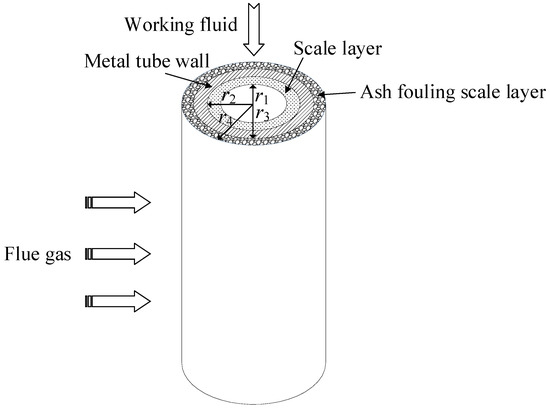
Figure 4.
Heat transfer of the low-temperature superheater tube wall.
Since the influence of is small, the effect of is ignored. Before the raw water is replenished into the boiler, the power plant must treat the boiler feed water to remove the salts, impurities and gases, so that the quality of the supply water meets certain requirements. Therefore, the thermal resistance of the scale layer is small and can be ignored to simplify the calculation of . Thus, the thermal resistance of the ash layer is calculated as follows, according to the Equation (8):
where the heat release coefficient of the flue gas side is the convective heat transfer coefficient and the radiation heat release coefficient , and is calculated as:
For the low-temperature convection heating surface, the radiation heat release coefficient . When tube bundles on the convection heating surface are arranged in parallel, the heat release coefficient on the flue gas side becomes
When the tube bundles on the convection heating surface are arranged in staggered rows, the convective heat transfer coefficient on the flue gas side is calculated as
The heat absorption coefficient on the working fluid side is given by
where ,,, are the correction factors determined by the structural dimensions of tube bundles, and represent the correction factor related to pipe pitch, the correction factor associated with the vertical tube row number, the correction factor related to airflow and wall temperature and the relative length correction factor, respectively; is the outer diameter of the low-temperature superheater tube; is the inner diameter of the low-temperature superheater tube; and are the flow rate of the working fluid and flue gas at the average temperature, respectively; and are the thermal conductivity of the working fluid and flue gas at the average temperature, respectively; and are the kinematic viscosity of the working fluid and flue gas at the average temperature, respectively; and are the dynamic viscosity of the working fluid and flue gas at the average temperature, respectively; and and are the constant-pressure specific heat of the working fluid and flue gas at the average temperature.
The thermal resistance of the ash layer is used to characterize the fouling degree of the convection heating surface. Generally, the larger the value is, the more serious the fouling of the heating surface is.
2.2. Wavelet Decomposition Model
In 1988, Mallat proposed a concept of multi-resolution with a fast algorithm for wavelet decomposition and reconstruction [29,30]. The original signal is a continuous wavelet. Then, the inner product of and , which is called the continuous wavelet transform, is described as
However, in actual engineering calculations, the signals are discrete. As a result, it is necessary to discretize the wavelet transform. The binary discrete wavelet transform (DWT) can be expressed as
The basic principle is as follows. A signal in space can be represented by basic functions in two orthogonal subspaces, and , which can be determined using Equation (16). According to Equation (17), the first level decomposes into a low-frequency part and a high-frequency part , the second level decomposes into a low-frequency part and a high-frequency part and so on, until the multi-resolution decomposition of signals can be realized.
In the scale metric space , the coefficient is decomposed to two wavelet coefficients and in the scale metric spaces and . Similarly, the two wavelet coefficients and can be used for reconstruction to get . The reconstruction algorithm and the decomposition algorithm are corresponding and mutually inverse.
2.3. VisuShrink Soft Threshold Denoising
Generally speaking, high-frequency signals contain noise details. The wavelet threshold denoising algorithm is an effective filtering method. After wavelet decomposition, the threshold wavelet method is used to weight the decomposed wavelet coefficients. For high-frequency wavelet coefficients, the VisuShrink soft threshold denoising method [31] is adopted for signal processing. All low-frequency wavelet coefficients representing the global trend of the original signal are retained. Then, all small signals are reconstructed to obtain denoising signals, as shown in Figure 5.
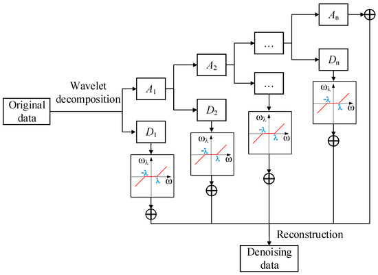
Figure 5.
Wavelet threshold denoising process.
The VisuShrink method selects the high-frequency wavelet coefficients to estimate the standard deviation of the noise:
The global threshold is determined as
Finally, the soft threshold denoising equation is written as follows
2.4. SVR Theory
An SVR [32,33,34] method is usually realized through regression and prediction. The principle of SVR is to learn a function , so that the function value is as close as possible to the real value. Given the training samples , with for the input, for the target output, as the number of training samples. The regression model equation is calculated as
where , ; , is kernel function. SVR transforms low-dimensional nonlinear problems into high-dimensional linear problems by introducing kernel functions. Solving the dual Lagrangian problem of SVR:
This is subject to
The above process must satisfy Karush–Kuhn–Tucker (KKT) conditions:
Eventually, the solution to SVR is
where is the kernel function.
The kernel function can map the nonlinear problem of low-dimensional space to high-dimensional space, which will then become a linear problem. However, constructing the kernel function is a significant problem. The most crucial step is to determine the mapping of input space to feature space, which can only be achieved if we know the distribution of data within the input space. However, in most cases, we do not know the specific distribution of data being processed. Therefore, it is generally challenging to construct a kernel function that conforms precisely to the input space, and as a result this paper uses the radial basis function (RBF) instead of rebuilding a new kernel function.
The Gaussian radial basis function is one of the most widely used kernel functions. It offers a better performance regardless of whether a sample is large or small, and it has fewer parameters than the polynomial kernel function. Therefore, the Gaussian kernel function is preferred in most cases.
Vapnike’s [35] research demonstrates that the kernel parameter and penalty factor are the key factors affecting the performance of SVM. A larger will reduce the training error, but will also result in over-fitting at the same time, which will increase the test error. When the kernel parameter is small, the regression prediction has better accuracy. However, if the kernel parameter is much lower, the accuracy of the model will drop significantly.
3. Case Study and Data Collection
This paper takes a 170 t/h tangentially fired pulverized coal boiler from the Huilian Power Plant in Wuxi, Jiangsu Province, China, as the research object. The horizontal section size of the furnace chamber is 7090 × 7090 mm (width × depth). Table 1 gives the design parameters of the boiler.

Table 1.
Design parameters of the boiler (rated load).
This type of case study boiler has a typical heating surface structure similar to that of many power station boilers in China. Figure 6 shows the schematic diagram of the case study boiler system. It can be seen that after the pulverized coal is burned by the furnace to produce flue gas, the flue gas flows along the flue gas passage all the way through the platen superheater, the high-temperature superheater, high-temperature reheater, low-temperature superheater, low-temperature reheater, economizer, air preheater and many other heating surfaces to the desulfurization tower and bag filter before finally being discharged by the chimney. The heat transfer mode of the heating surfaces is convection, except for the platen superheater which is half radiation and half convection. In the actual operation of the boiler, the flue gas contains a large number of fly ash particles. When fly ash is deposited on the heated surface, the heat transfer performance is degraded.
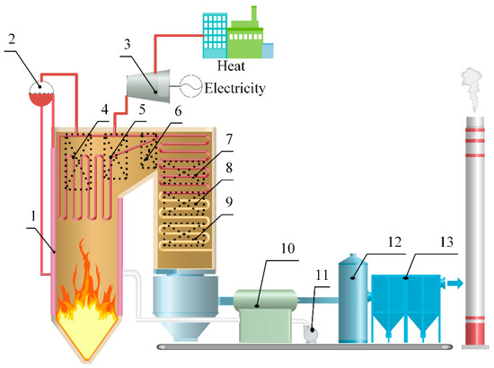
Figure 6.
Schematic diagram of the boiler system case study. 1—water wall, 2—steam-water separator, 3—steam turbine, 4—platen superheater, 5—high-temperature superheater, 6—high-temperature reheater, 7—low-temperature superheater, 8—low-temperature reheater, 9—economizer, 10—air preheater, 11—air blower, 12—desulfurization tower, 13—bag filter.
The data used in this study was collected from the DCS of power plants, as shown in Table 2. By analyzing the formation mechanism and influence factors of ash fouling, 20 characteristic parameters affecting the ash fouling were selected, including the eight powder feeder speeds, the main steam flow rate, the main steam pressure, the main steam temperature, the outlet steam temperature, the inlet flue gas temperature, the outlet flue gas temperature, the steam flow rate, the feedwater flow rate, the feedwater temperature, the boiler oxygen amount, the air supply rate of blower A and the air supply rate of blower B. The function of the powder feeder is to continuously and uniformly send pulverized coal from the pulverized coal bin to the furnace for combustion according to the coal burning amount required by the boiler load. The speed can control the amount of pulverized coal entering the furnace. Blower A is a primary fan of the boiler that is used to dry the fuel and send it into the furnace. Blower B is a secondary fan of the boiler that is used to overcome resistance from the air preheater, air duct and burner, and to maintain full combustion of fuel. The air blowers are located at the air inlet of the air preheater (Figure 6, number 11). In summary, this paper uses 20 characteristic parameters that formed the input set of the SVR model. The input data were collected every three minutes from 25 May 2019 at 00:00 to 29 May 2019 at 23:57. After the normalization of these 2400 sets of data, all samples were divided into an 80% training set and a 20% test set.
In this study, the thermal resistance of the ash layer was chosen to be an indicator by which to detect the degree of fouling on the heated surface. After the original thermal resistance data were de-noised by wavelet analysis, the focus was to set up correlations between the 20 characteristic parameters and the thermal resistance of the ash layer using the SVR model.
4. Results and Discussion
4.1. Analysis of the Ash-Layer Thermal Resistance
Taking advantage of the thermal resistance mechanism model for the low-temperature superheater established in Section 2.1, the thermal resistance of the ash layer combined with the operation data from the Huilian power plant was calculated. Figure 7 is the calculation result of the ash-layer thermal resistance for the low-temperature superheater. The smaller the thermal resistance of ash-layer value, the better the heat transfer performance of the low-temperature superheater was.
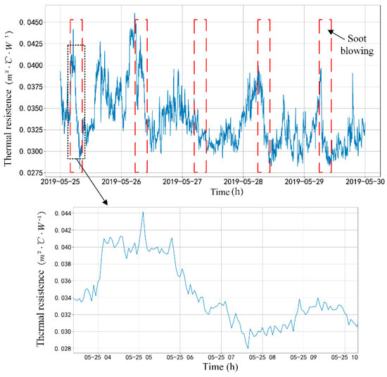
Figure 7.
The changing trend of the thermal resistance for the low-temperature superheater.
It can be seen that there was a sudden drop every day from 06:00–08:00 as the result of a scheduled ash blowing operation by the power plant, and that the thermal resistance of the ash layer of the heating surface decreased significantly after soot blowing.
On the morning of 27 May 2019, the degree of ash fouling on the heating surface was not serious enough, but the operator still performed the blowing operation, which exposed the shortcomings of the scheduled soot blowing action. Scheduled soot blowing does not consider whether ash accumulation is severe, and wastes steam that causes severe pipe wall wear, resulting in a decrease in boiler efficiency. The improper operation of the soot blower will not only reduce the economic benefit of unit operation, but will also lead to pipe wall wear or even an explosion of the pipe, affecting the safety of the boiler unit.
This paper calculates the thermal resistance of the ash layer in order to observe and visualize degrees of ash fouling on the heating surface. Based on quantification, the original soot blowing method can be changed from scheduled soot blowing to on-demand soot blowing.
On the other hand, it can be observed that there are a large number of sawtooth fluctuations in Figure 7. These were caused by noise data and unstable working conditions during operations. Changes in working conditions can affect the heat transfer performance of the heating surface. These fluctuations are very unfavorable for both the operator’s observations and the development of an ash blowing strategy.
4.2. Wavelet Threshold Denoising Results
The wavelet threshold denoising algorithm was performed to smooth and filter the thermal resistance data, reducing the influence of sawtooth fluctuations on the degree of ash fouling. This method not only preserved the changing trend of thermal resistance, but also lessened the sawtooth jitter. It also provided cleaner raw data for the next training of the SVR model.
In this experiment, the sym5 wavelet was selected with two to five decomposition levels. Figure 8 shows the waveform diagram for each high-frequency and low-frequency signal after wavelet decomposition. The comparison results for the two to five wavelet decomposition levels and the denoising are shown in Figure 9a–d.
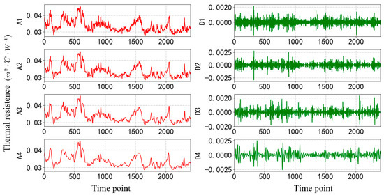
Figure 8.
Results of four-level wavelet decomposition using the sym5 wavelet.
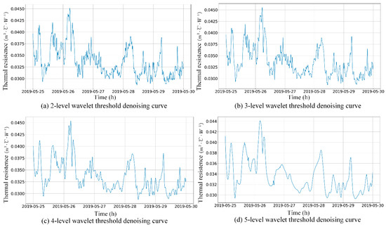
Figure 9.
Wavelet threshold denoising results.
The signal-to-noise ratio (SNR) and root mean square error (RMSE) are shown after denoising in Table 3, which demonstrates the accurate quantization of the denoising effect. The higher the SNR of the signal, the smaller the RMSE, and the closer the denoising signal was to the original signal. It can be seen that the denoised curve not only retained the changing trend of the original signal, but also eliminated the influence of partial noises.
Table 3.
Root mean square error (RMSE) and signal-to-noise ratio (SNR) of wavelet denoising signals with different levels.
It can be seen in Figure 9 and Table 3 that after calculation with the four-level wavelet threshold denoising algorithm, the results of SNR and RMSE were 31.8 and 0.000865, respectively. This indicates that thermal resistance data after a four-level wavelet threshold denoising filtering not only maintained the overall trend, but also reduced sawtooth fluctuations to a minimum. Thus, the wavelet threshold denoising algorithm was rendered valid by filtering out some noise information.
However, the five-level wavelet threshold denoising lost some of the details of the original signal, thus the four-level wavelet threshold denoising results were applied as the output data sets of the SVR model described in Section 2.4. After wavelet decomposition and denoising, the changing trend of thermal resistance was more visible, which is more conducive to the design of blowing ash optimization strategy.
4.3. Fouling Prediction Based on SVR
The SVR model described in Section 2.4 was utilized for training the mapping relationship between characteristic parameters and the thermal resistance of the ash layer. The grid search method was adopted to optimize the two hyper-parameters of the SVR, including penalty factor and kernel parameter .
Predictive simulation experiments were performed in the Python 3.6 environment. The first 80% of samples were divided into a training set and the remaining 20% into a testing set. The RBF kernel function was then presented. The performance evaluation criterion selected for the SVR model was the coefficient of determination (optimum was the maximum value). The grid search method was used for hyper-parametric optimization to improve the prediction accuracy of the SVR model. Figure 10 shows the model prediction accuracy under different hyper-parameters . Training and testing accuracy of the SVR model using four-level wavelet decomposition and denoising data are provided in Table 4. The optimum hyper-parameters of the SVR model were (29, 0.13), and the accuracy of the training set and testing set were 0.994 and 0.985, respectively.
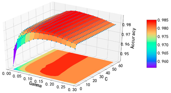
Figure 10.
Prediction accuracy with different hyper-parameters based on the grid search algorithm.
Table 4.
Training and testing accuracy of the SVR model by using the four-level wavelet decomposition denoising signal.
The output results for the thermal resistance of the ash layer were predicted by simulating the SVR model and comparing it with the actual results of the mechanism model. The original data and forecasted data of the thermal resistance for the training and testing phases are illustrated in Figure 11. Figure 12 is a graph of the absolute error residual. It can be observed that the predicted value of the SVR model was within a range of ±5% of the actual value of the mechanism model, as shown in Figure 13.
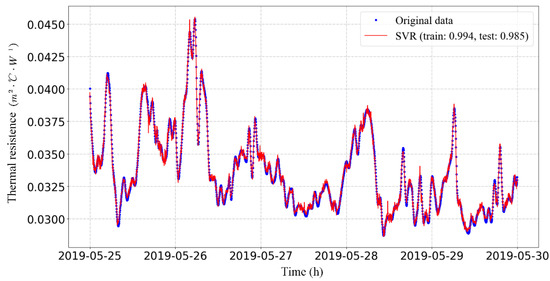
Figure 11.
Comparison between the original value and the predicted value of thermal resistance.
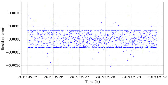
Figure 12.
Absolute error diagram of prediction results.
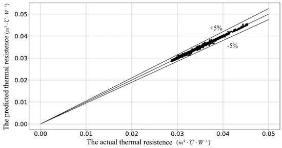
Figure 13.
Comparison of predicted and actual thermal resistance.
The SVR model can predict the fouling process of the heating surface with precision by using 20 characteristic parameters and avoiding the establishment of complex equations such as heat transfer and radiation. The ash fouling prediction model of boiler heating surfaces based on wavelet analysis and SVR has good generalization and can meet the actual soot blowing operation requirements.
5. Conclusions
In this study, a thermal resistance network of the ash layer is developed to characterize the degree of boiler ash fouling for the first time, and a physical model was established based on the heat transfer balance principle of the low-temperature superheater. To reduce the adverse effects of sawtooth fluctuations, a method based on wavelet analysis and SVR was proposed to improve the online prediction of thermal resistance. The case study showed that the SNR and RMSE obtained using a four-level wavelet threshold denoising algorithm to filter the thermal resistance data were 31.8 and 0.000865, respectively. This indicates that the filtered thermal resistance data not only maintained the overall trend, but also reduced the sawtooth fluctuation to a minimum. With the filtered thermal resistance data, an SVR model was trained to map the relationship between characteristic parameters and the thermal resistance of the ash layer. The maximum prediction accuracy was 99.4% during the training phase and 98.5% during the testing phase. The accuracy of this method can meet real engineering needs and provide an innovative way for the analysis and prediction of ash accumulation for a low-temperature superheater.
The wavelet analysis and SVR model make it possible to predict ash fouling online without significant sawtooth fluctuation. Therefore, considering the degree of agreement between the predicted results and the actual calculated results, the online prediction method of thermal resistance based on wavelet analysis and SVR can be used as an appropriate prediction tool for estimating and predicting the ash fouling behavior of a low-temperature superheater without adding complicated and expensive equipment.
Author Contributions
Conceptualization, S.T. and X.Z.; data curation, Y.W.; investigation, N.T.; methodology, X.Z and W.Z.; software, X.Z; supervision, S.T. and Z.T.; validation, X.Z., Z.T. and N.T.; visualization, Y.W.; writing—original draft, S.T., X.Z., Z.T. and W.Z.; writing—review and editing, S.T., X.Z., Z.T. and W.Z. All authors have read and agreed to the published version of the manuscript.
Funding
This work was supported by the National Key R & D Program of China (Grant No. 2017YFA0700305 and 2018YFB0606105), Zhejiang Provincial Natural Science Foundation (Grant No. LR19E050002, LY17F030007), and Zhejiang University & Huaguang Smart Energy System Joint Research Center.
Acknowledgments
We are very grateful for the contributions of Jianyun Zhao from Hangzhou Boiler Group Co., Ltd., Hangzhou, China, Junhua Mao from Wuxi Huaguang Boiler Co., Ltd., Wuxi, China, Liangwei Xia from Harbin Boiler Co., Ltd., Harbin, China, and Wen Yang from Jianglian Heavy Industry Group Co., Ltd., Nanchang, China. These industrial collaborators mentioned above made significant contributions to this paper although they were not co-authored.
Conflicts of Interest
The authors declare no conflict of interest.
Nomenclature
| Acronyms | heat release coefficient of the flue gas side () | ||
| ANN | artificial neural network | heat absorption coefficient of the working fluid side () | |
| DCS | distributed control system | ash-layer thermal conductivity () | |
| DWT | discrete wavelet transform | metal tube thermal conductivity () | |
| KKT | Karush Kuhn Tucker conditions | scale-layer thermal conductivity () | |
| PSO | particle swarm optimization | inner radius of the scale layer () | |
| RBF | radial basis function | inner radius of the metal tube () | |
| RMSE | root mean square error | outer radius of the metal tube () | |
| SNR | signal-to-noise ratio | outer radius of the ash layer () | |
| SVM | support vector machine | length of the metal tube () | |
| SVR | support vector regression | thermal resistance of the ash layer () | |
| Symbols | thermal resistance of the metal tube () | ||
| convection heat absorption of the working fluid side () | thermal resistance of the scale layer () | ||
| convection heat release of the flue gas side () | correction factor related to pipe pitch | ||
| quantity of the working fluid flow () | correction factor related to the vertical tube row number | ||
| calculating fuel quantity () | correction factor related to airflow and wall temperature | ||
| enthalpy of inlet working fluid () | relative length correction factor | ||
| enthalpy of outlet working fluid () | outer diameter of the low-temperature superheater tube () | ||
| enthalpy of inlet flue gas () | inner diameter of the low-temperature superheater tube () | ||
| enthalpy of outlet flue gas () | flow rate of the working fluid at the average temperature () | ||
| the reduced value of steam enthalpy in the desuperheater () | flow rate of the flue gas at the average temperature () | ||
| heat retention coefficient | thermal conductivity of the working fluid at the average temperature () | ||
| air leakage coefficient | thermal conductivity of the flue gas at the average temperature () | ||
| theoretical cold air enthalpy () | kinematic viscosity of the working fluid at the average temperature () | ||
| superheated steam enthalpy () | kinematic viscosity of the flue gas at the average temperature () | ||
| superheated steam pressure () | dynamic viscosity of the working fluid at the average temperature () | ||
| the difference between the inlet temperature of the flue gas side and the inlet temperature of the working fluid side () | dynamic viscosity of the flue gas at the average temperature () | ||
| the difference between the outlet temperature of the flue gas side and the outlet temperature of the working fluid side () | constant-pressure specific heat of the working fluid at the average temperature () | ||
| heat transfer area of the low-temperature superheater () | constant-pressure specific heat of the flue gas at the average temperature () | ||
References
- Tong, Z.; Cheng, Z.; Tong, S. Preliminary Design of Multistage Radial Turbines Based on Rotor Loss Characteristics under Variable Operating Conditions. Energies 2019, 12, 2550. [Google Scholar] [CrossRef]
- Zhang, Y.; Bo, X.; Zhao, Y.; Nielsen, C.P. Benefits of current and future policies on emissions of China’s coal-fired power sector indicated by continuous emission monitoring. Environ. Pollut. 2019, 251, 415–424. [Google Scholar] [CrossRef] [PubMed]
- Li, J.; Zhang, Y.; Tian, Y.; Cheng, W.; Yang, J.; Xu, D.; Wang, Y.; Xie, K.; Ku, A.Y. Reduction of carbon emissions from China’s coal-fired power industry: Insights from the province-level data. J. Clean. Prod. 2019, 242, 118518. [Google Scholar] [CrossRef]
- Du, M.; Wang, X.; Peng, C.; Shan, Y.; Chen, H.; Wang, M.; Zhu, Q. Quantification and scenario analysis of CO2 emissions from the central heating supply system in China from 2006 to 2025. Appl. Energy 2018, 225, 869–875. [Google Scholar] [CrossRef]
- Lu, Y.; Zhao, S. Discussion on Approach to Renovation of Industrial Coal-Fired Boilers in China. J. Environ. Account. Manag. 2015, 3, 23–30. [Google Scholar] [CrossRef]
- Tong, S.; Huang, Y.; Jiang, Y.; Weng, Y.; Tong, Z.; Tang, N.; Cong, F. The identification of gearbox vibration using the meshing impacts based demodulation technique. J. Sound Vib. 2019, 461, 114879. [Google Scholar] [CrossRef]
- Dong, M.; Li, S.; Xie, J.; Han, J. Experimental studies on the normal impact of fly ash particles with planar surfaces. Energies 2013, 6, 3245–3262. [Google Scholar] [CrossRef]
- Bilirgen, H. Slagging in PC boilers and developing mitigation strategies. Fuel 2014, 115, 618–624. [Google Scholar] [CrossRef]
- Shi, Y.; Wen, J.; Cui, F.; Wang, J. An Optimization Study on Soot-Blowing of Air Preheaters in Coal-Fired Power Plant Boilers. Energies 2019, 12, 958. [Google Scholar] [CrossRef]
- Shi, Y.; Li, Q.; Wen, J.; Cui, F.; Pang, X.; Jia, J.; Zeng, J.; Wang, J. Soot Blowing Optimization for Frequency in Economizers to Improve Boiler Performance in Coal-Fired Power Plant. Energies 2019, 12, 2901. [Google Scholar] [CrossRef]
- Chen, Y.; Tong, Z.; Wu, W.; Samuelson, H.; Malkawi, A.; Norford, L. Achieving natural ventilation potential in practice: Control schemes and levels of automation. Appl. Energy 2019, 235, 1141–1152. [Google Scholar] [CrossRef]
- Hu, J.; Tong, Z.; Xin, J.; Yang, C. Simulation and experiment of a remotely operated underwater vehicle with cavitation jet technology. J. Zhejiang Univ.-Sci. A 2019, 20, 804–810. [Google Scholar] [CrossRef]
- Zhang, S.P.; An, L.S.; Shen, G.Q.; Niu, Y.G. Acoustic Pyrometry System for Environmental Protection in Power Plant Boilers. J. Environ. Inform. 2014, 23. [Google Scholar] [CrossRef]
- Zhang, S.; Shen, G.; An, L.; Li, G. Ash fouling monitoring based on acoustic pyrometry in boiler furnaces. Appl. Therm. Eng. 2015, 84, 74–81. [Google Scholar] [CrossRef]
- Shi, Y.; Wang, J.; Liu, Z. On-line monitoring of ash fouling and soot-blowing optimization for convective heat exchanger in coal-fired power plant boiler. Appl. Therm. Eng. 2015, 78, 39–50. [Google Scholar] [CrossRef]
- Zhang, X.; Yuan, J.; Chen, Z.; Tian, Z.; Wang, J. A dynamic heat transfer model to estimate the flue gas temperature in the horizontal flue of the coal-fired utility boiler. Appl. Therm. Eng. 2018, 135, 368–378. [Google Scholar] [CrossRef]
- Trojan, M.; Taler, D. Thermal simulation of superheaters taking into account the processes occurring on the side of the steam and flue gas. Fuel 2015, 150, 75–87. [Google Scholar] [CrossRef]
- Sivathanu, A.K.; Subramanian, S. Extended Kalman filter for fouling detection in thermal power plant reheater. Control Eng. Pract. 2018, 73, 91–99. [Google Scholar] [CrossRef]
- Sobota, T. Improving Steam Boiler Operation by On-Line Monitoring of the Strength and Thermal Performance. Heat Transf. Eng. 2018, 39, 1260–1271. [Google Scholar] [CrossRef]
- Pronobis, M. The influence of biomass co-combustion on boiler fouling and efficiency. Fuel 2006, 85, 474–480. [Google Scholar] [CrossRef]
- Feng, H.; Zhong, W.; Wu, Y.; Tong, S. Thermodynamic performance analysis and algorithm model of multi-pressure heat recovery steam generators (HRSG) based on heat exchangers layout. Energy Convers. Manag. 2014, 81, 282–289. [Google Scholar] [CrossRef]
- Tong, Y.; Zhong, W.; Wu, Y.L.; Tong, S.G. The study on heat transfer model and algorithm of multi-sectional regenerative air heater in power plant boiler based on analytical method. Appl. Mech. Mater. 2014, 448, 3229–3233. [Google Scholar] [CrossRef]
- Feng, H.C.; Zhong, W.; Wu, Y.L.; Tong, S.G. The Effects of Parameters on HRSG Thermodynamic Performance. Adv. Mater. Res. 2013, 774, 383–392. [Google Scholar] [CrossRef]
- Teruel, E.; Cortes, C.; Diez, L.I.; Arauzo, I. Monitoring and prediction of fouling in coal-fired utility boilers using neural networks. Chem. Eng. Sci. 2005, 60, 5035–5048. [Google Scholar] [CrossRef]
- Peña, B.; Teruel, E.; Diez, L.I. Soft-computing models for soot-blowing optimization in coal-fired utility boilers. Appl. Soft Comput. 2011, 11, 1657–1668. [Google Scholar] [CrossRef]
- Mohanty, D.K.; Singru, P.M. Fouling analysis of a shell and tube heat exchanger using local linear wavelet neural network. Int. J. Heat Mass Transf. 2014, 77, 946–955. [Google Scholar] [CrossRef]
- Sun, L.; Zhang, Y.; Saqi, R. Research on the fouling prediction of heat exchanger based on Support Vector Machine optimized by particle swarm optimization algorithm. In Proceedings of the 2009 International Conference on Mechatronics and Automation, Changchun, China, 9–12 August 2009; pp. 2002–2007. [Google Scholar]
- Smola, A.J.; Schölkopf, B. A tutorial on support vector regression. Stat. Comput. 2004, 14, 199–222. [Google Scholar] [CrossRef]
- Mallat, S.G. A theory for multiresolution signal decomposition: The wavelet representation. IEEE Trans. Pattern Anal. Mach. Intell. 1989, 11, 674–693. [Google Scholar] [CrossRef]
- Daubechies, I. Orthonormal bases of compactly supported wavelets. Commun. Pure Appl. Math. 1988, 41, 909–996. [Google Scholar] [CrossRef]
- Donoho, D.L.; Johnstone, J.M. Ideal spatial adaptation by wavelet shrinkage. Biometrika 1994, 81, 425–455. [Google Scholar] [CrossRef]
- Drucker, H.; Burges, C.J.C.; Kaufman, L.; Smola, A.J.; Vapnik, V. Support vector regression machines. In Advances in Neural Information Processing Systems 9; MIT Press: Cambridge, MA, USA, 1997; pp. 155–161. [Google Scholar]
- Basak, D.; Pal, S.; Patranabis, D.C. Support vector regression. Neural Inf. Process. Rev. 2007, 11, 203–224. [Google Scholar]
- Gunn, S.R. Support Vector Machines for Classification and Regression; ISIS Technical Report; University of Southampton: Southampton, UK, 1998; Volume 14, pp. 5–16. [Google Scholar]
- Chapelle, O.; Vapnik, V.; Bousquet, O.; Mukherjee, S. Choosing multiple parameters for support vector machines. Mach. Learn. 2002, 46, 131–159. [Google Scholar] [CrossRef]


© 2019 by the authors. Licensee MDPI, Basel, Switzerland. This article is an open access article distributed under the terms and conditions of the Creative Commons Attribution (CC BY) license (http://creativecommons.org/licenses/by/4.0/).