Abstract
The environment for practical applications of an energy storage system (ESS) in a microgrid system is very harsh, and therefore actual operating conditions become complex and changeable. In addition, the signal of the ESS sampling process contains a great deal of system and measurement noise, the sampled current fluctuates significantly, and also has high frequency. In this case, under such conditions, it is difficult to accurately estimate the state of charge (SOC) of the batteries in the ESS by common estimation methods. Therefore, this study proposes a compound SOC estimation method based on wavelet transform. This algorithm is very suitable for microgrid systems with large current, frequent fluctuating conditions, and high noise interference. The experimental results and engineering data show that the relative error of the method is 0.5%, which is much lower than the extend Kalman filter (EKF) based on wavelet transform.
1. Introduction
Generally, microgrid, is a system unit consisting of a load and a micro power supply that can provide power and heat at the same time to meet the user’s requirements for power quality and power supply safety as compared with an external large power grid, which is a single controlled unit. The power supply inside the microgrid is mainly responsible for energy conversion by power electronic devices, and provides the necessary control.
As a critical energy storage component, electrochemical batteries are sometimes used to store or release energy in the energy storage system (ESS). They are a good choice to improve the reliability, flexibility, and stability of the microgrid, especially in smoothing the randomness and volatility of the renewable energy generation [1,2,3], ensuring the important loads operate normally during power shortage or large external power grid failure [4,5], helping to cut peak and fill valley of time-of-use electricity price [6], and increasing the local consumption rate and energy permeability of renewable energy.
Currently, the electrochemical battery ESS is divided into lead-acid battery, lead carbon battery, lithium-ion battery, sodium-sulfur battery, and liquid flow battery. Lead carbon batteries are less costly than lithium-ion, flow, and sodium-sulfur batteries, and in partial state of charge (PSoC) cycle tests, a charging rate below 1 C and ohmic efficiency of 91% to 94% can reach 99.9% [7]. Additionally, as compared with lead-acid battery, the charge or discharge reaction of lead carbon battery is much easier at a high-rate partial state of charge (HRPSoC) condition, with longer cycle life and higher charging acceptability [8,9]. The lead carbon battery is a new type of energy storage battery, which is formed by adding carbon material to the negative electrode plate of the lead-acid battery.
In addition, the PSoC operation mode enhances charge efficiency and reduces material degradation caused by overcharge [8,9,10], which is the preferred operation mode of lead carbon batteries.
In a lead carbon battery energy storage system (BESS), a battery management system (BMS) monitors and manages the batteries and extends the life, as well as improves the stability of the ESS [11,12]. State of charge (SOC) is a necessary parameter in the BMS. It provides important information for the residual energy of the ESS and an important basis for the management and maintenance of the ESS. Overcharging and over-discharging leads to a decline in battery life, or even combustion or explosion. Therefore, monitoring the SOC of the battery is an essential task of BMS. A precise SOC is important to the safe and stable working of the ESS. In an actual project of ESS, the capacity, the operating environment, and the cycle times of the battery all affect the precision of the SOC estimation.
As a core technology, SOC estimation algorithms have been studied widely. In the early stage of research, frequently used methods have been the open circuit voltage (OCV) algorithm and the ampere-hour integral (Ah) method. The OCV algorithm [13] estimates SOC by establishing the relationship function between OCV and SOC, which is the measured terminal voltage after the battery is static for a period of time. The static time has different requirements according to the type of battery. The (Ah) method [14] estimates the SOC by integrating the current of the cell with time. However, since the initial value of SOC is unknown, it belongs to an open-loop calculation in the estimation process of the algorithm, and the accuracy is affected by the initial value.
These methods are easily implemented and applied in engineering. In recent years, researchers at home and abroad have put forward many complicated methods to estimate SOC. For example, the extend Kalman filter (EKF) method is suitable for SOC estimation with relatively intense fluctuations of the current. It overcomes some shortcomings of the methods in earlier researches but requires higher accuracy of the battery model [15]. A new intelligent algorithm, BP neural network method, does not need to establish an accurate mathematical model, however this method needs a lot of experimental data for training, and the more training data, the higher the accuracy and the longer the time required [16]. As compared with other methods, the SVM algorithm has better robustness and faster iterative computing speed. However, the accuracy of the estimation depends on the selection of support vector regression (SVR) parameters, and the estimation accuracy is reduced substantially if the parameter combination is not optimal [17].
In summary, each algorithm has its own merits and demerits. In this study, the composite algorithm is proposed, fused with wavelet transform, the Ah method, the OCV method, and the EKF algorithm, which combine the advantages of all the algorithms suitable for the working conditions in this field of ESS in microgrid systems. This algorithm decomposes the measured signal, then, selects thresholds to denoise the original signal which is obtained by wavelet reconstruction, and, then, carries out the EKF algorithm on every scale. The detailed steps of the algorithm are outlined in the Section 3 of this paper. In order to adopt the EKF method, a discrete-time state-space model must be established. The model and the parameters are discussed in Section 2 of this paper.
2. Cell Model and Parameters
2.1. Cell Model
SOC can be defined as follows:
It indicates the ratio between the usable capacity of the battery and the current maximum capacity of the battery. The original value is , the load current is , the Coulomb efficiency is which is related to and obtained by Equation (8), and the maximum capacity is .
At present, there are many types of battery models [18,19]. Figure 1 demonstrates the second-order (resistance- capacitance) RC model, which describes the charge and discharge characteristics of the battery.
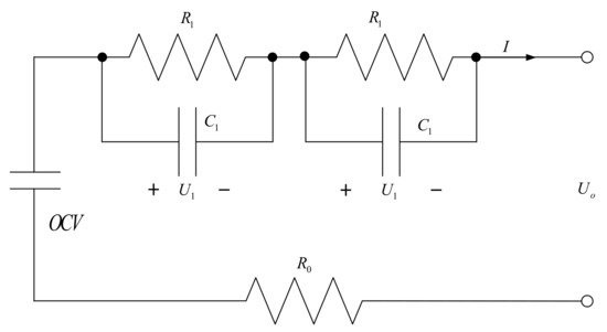
Figure 1.
Second-order RC cell model.
Where is open circuit voltage, is ohmic resistance, is electrochemical polarization resistance; is concentration polarization resistance, is electrochemical polarization capacitance, is concentration polarization capacitance, is charging/discharging current, and is terminal voltage. The relationships among these parameters are as follows:
where and are the voltages of and , OCV is measured as a function of the SOC through the following experiment.
In order to use the EKF algorithm to estimate SOC, the state-space equations of a battery need to be established, which are established by deriving Equation (1) and combining it with Equations (2) to (4). The equations are as follows:
2.2. Experiments
The setup of the experiments is shown in Figure 2. The experimental object is lead carbon batteries, whose characteristics are shown in Table 1. The Chroma 17020 device controled the batteries charging and discharging, and the host computer was used to record and analyze the parameters’ information of the battery. The experiments were carried out under constant temperature, which was 25 °C, to prevent the interference caused by temperature. The batteries used in the experiments were produced from the same batch, which are all brand new, to prevent the interference of inconsistency and self-discharge.
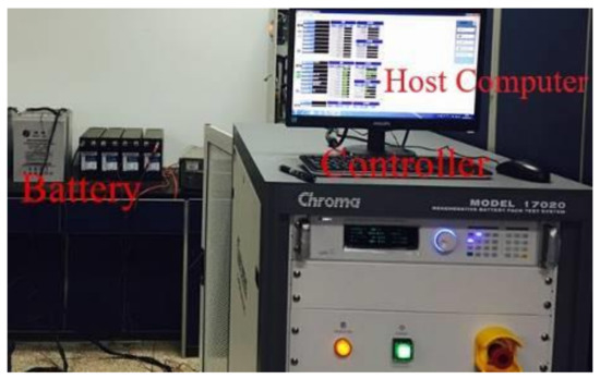
Figure 2.
Experimental device.

Table 1.
The lead carbon battery characteristics.
The first experiment was conducted to build the function between OCV and SOC. First, batteries were discharged at a constant current of 0.2 C and 0.4 C from 100% to 0% with an interval of 10% SOC. After each discharged pulse, a 3 h static time was considered to identify the OCV. The second step was to perform a similar test with constant currents of 0.2 C and 0.4 C, with the batteries charging state being 10% and charging from 0% to 100%. The OCV was obtained at every 10% of the SOC after every 3 h rest period. Finally, the last step was to obtain the relationship curves between OCV and SOC.
The functional relationship between the Coulomb efficiency and the load instantaneous current was obtained through the second test.
The discharge efficiency was obtained by the following steps:
The batteries are charged at a current of 0.1 C in constant current (CC) mode until the voltage reached a floating charge voltage of 2.2 V, and, then, charged in constant voltage (CV) mode until the current was less than 0.01 C. At that time, the battery was considered fully charged. Next, the batteries were discharged in CC mode until the voltage reached the cut-off voltage of 1.8 V. At this time, the battery was considered empty. This experiment needs to be charged in CCCV mode at a current of 0.1 C after each discharge. However, the discharge current was different, which was 0.1 C, 0.2 C, 0.3 C, 0.4 C, 0.5 C, and 0.6 C, respectively, and therefore the discharge efficiency was calculated under different current.
The charge efficiency was obtained as follows:
It is different from the last experiment in that the charge current is different (0.1 C, 0.2 C, 0.3 C, 0.4 C, 0.5 C, and 0.6 C, respectively) while the discharge current (0.1 C) was the same. Therefore, the charge efficiency was calculated under different current.
2.3. Parameters Identification
2.3.1. Acquisition of OCV
The curve of average values is obtained by calculating the 0.2 C and 0.4 C SOC-OCV average values from the first experiment. The current of 0.2 C and 0.4 C are common in practical application conditions, and the average value represents the SOC-OCV relationship. The final curves are shown in Figure 3.
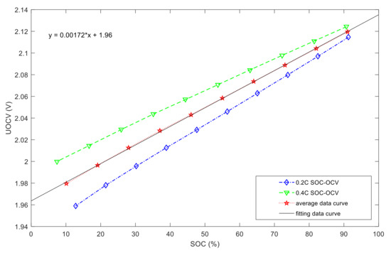
Figure 3.
The state of charge and open circuit voltage (SOC-OCV) functional relationship curves.
The OCV is measured as a function of the SOC, and the equation of the linear fitting curve of the average data is shown as follows:
2.3.2. Acquisition of
The charge and discharge efficiency were acquired from the second test. Table 2 summarizes the experimental data. The curves are shown in Figure 4. The curve of average efficiency values is obtained by calculating the charge efficiency and the discharge efficiency values.
Table 2.
The current rate and efficiency relationship.
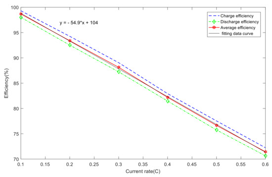
Figure 4.
The current rate and efficiency functional relationship curves.
The equation of the linear fitting curve of the average efficiency values is shown as follows:
where is the average efficiency and is the current rate which is easily obtained by the current.
2.3.3. Acquisition of Other Parameters
is identified by voltage sag data at the moment of power failure. The parallel RC circuit simulates the transient dynamics of the battery, which is an inertial delay link. The parameters are identified by nonlinear fitting of zero-input data in the static state of batteries. The identification results are shown in Table 3.
Table 3.
Relationship of parameters and different SOC.
The parameters of the model, as shown in Table 3, are changing with SOC. If the parameters of the model are obtained by the look-up table method, the error of SOC estimation is related to the amount of data in the table, and this method needs to provide a large number of experiments, which is more cumbersome. At present, online identification of model parameters is proposed, which can accurately estimate SOC. It can be realized by the following Equations (9) to (14) [20].
where , , , , is the initial value of , , , , in different SOC, , , , , are the first-order coefficient and , , are the second-order, is the measured value of voltage, and is the estimated value of voltage.
The results of and are shown in Figure 5. The solid line is the experimental data of the battery voltage, while the dotted line is the voltage data calculated through the battery model, as has been described above. Figure 6 is the relative error analysis (the experimental data and the calculated data). It can be seen from the Figure 6 that the estimated data is consistent with the measured data, and most error data is within 0.8%, except for two individual points. The error is relatively large at the end of the experiment, which is due to the fact that the battery model used in this study does not consider the influence of temperature, and the accuracy of estimation needs to be improved.
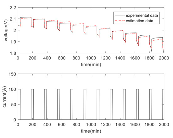
Figure 5.
Experimental data and estimation data.
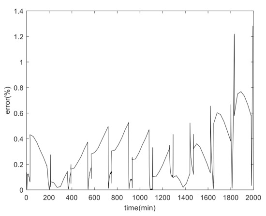
Figure 6.
Analysis of voltage.
3. SOC Estimation
Wavelet transform provides qualitative analysis in time and frequency domain, as is often used for signal and image denoising [21,22,23]. The BMS sensors are easily affected by interference from converters and signal transmission lines while they are sampling data such as current, voltage, and temperature. The measured signal contains noise, most of which has time-varying complexity and obey Gaussian distribution. After the completion of wavelet transform, the signal still obeys Gaussian distribution at all scales, which satisfies the condition of EKF estimation.
3.1. Denoising Approach
According to the characteristics of wavelet transform, a threshold denoising method in wavelet domain is proposed. After sampling the original voltage and current signals, they are decomposed by 2n order wavelet transform matrix (WTM). In the process of denoising, the wavelet coefficients are adjusted according to the threshold rules. Then, the denoised current and voltage signals are reconstructed by using these denoised wavelet coefficients and 2n order inverse wavelet transform matrix (IWTM).
3.1.1. Decomposition of Original Signals
A time domain signal is decomposed into a different frequency signal by discrete wavelet transform (DWT), which contains the approximations and the details.
The wavelet transform mainly focuses on the finite coefficients in the wavelet domain and the coefficients amplitude is large. The wavelet coefficients of noise are distributed in the entire wavelet domain, and the amplitude is small. Therefore, we quantify the wavelet coefficients by choosing appropriate thresholds on different scales, eliminating smaller wavelet coefficients, and retaining larger wavelet coefficients, and therefore the noise in the signal is suppressed. Finally, the optimal estimation of the real signal is obtained by inverse wavelet transform matrix (IWTM).
In order to analyze the original signals, a decomposition method based on wavelet transform matrix (WTM) is used to decompose the collected battery voltage and current signals.
The sampled current and voltage signals are expressed as the following matrices:
where and are matrices of the voltage and current of batteries.
The -level decomposition process is as follows:
where and are the voltage and current signals approximation coefficients, and are the voltage and current signals detail coefficients. and are matrices of the decomposed wavelet coefficients.
3.1.2. Selecting Threshold for Denoising
In order to remove the noise, the wavelet coefficients mentioned above need to be adjusted according to the threshold rules [23,24,25]. At -level, the threshold value needs to be satisfied
is the length of the signal and is the standard variance of noise signal.
Generally speaking, the commonly used threshold functions contain hard threshold function and soft threshold function.
The hard threshold function is described by Equation (19). If the wavelet coefficients absolute value is bigger than or equal to the threshold value , all of them are preserved; if the is smaller than the , all of them are set to zero.
Equation (20) is the expression of soft threshold function. If the is bigger than or equal to the , the difference between both is taken as the new wavelet coefficients. If the is smaller than the , all the wavelet coefficients are set to zero.
The hard threshold preserves the mutation information, whereas the soft threshold processes signals relatively smoother, leading to such distortion as blurred edge. In order to overcome the above shortcomings, a combination of soft threshold and hard threshold of the prior knowledge of noise is proposed, which makes use of the best advantages of both hard and soft threshold. By adding an adjustment coefficient (), the estimated wavelet threshold is between the hard threshold function and the soft threshold function, which is closer to the real wavelet coefficients. Its expression is as follows:
The denoised wavelet coefficients of voltage and current is acquired by adjusting the coefficients according to the threshold rules.
where and are matrices of denoised wavelet coefficients. , are the denoised detail coefficients.
3.1.3. Denoised Signal Obtained by Wavelet Reconstruction
Finally, the optimal estimation of the real signal is obtained by IWTM.
where and are matrices of denoised voltage and current signals.
Wavelet denoising is mainly affected by threshold selection, decomposition level, and wavelet base selection. Generally, the decomposition layers are three to five layers; being too large or too small affects the quality of denoising [26,27]. Among these three factors, the key is to select threshold and quantify threshold, directly affecting the quality of signal denoising. The soft thresholding method reduces the modulus of wavelet coefficients. After noise reduction, the signal is smooth but the mutation information becomes fuzzy. However, the hard thresholding method retains the mutation information of the signal, although the signal is possibly not smooth enough after noise reduction.
In this study, a wavelet denoising method is used based on the combination of soft threshold and hard threshold of prior knowledge. The hard threshold method is used for the frequency band with large energy of useful signal components, whereas the soft threshold method is used for the frequency band with small energy of useful signal components. Determined by the energy and amplitude of the noise, the method of threshold selection is simulated and verified by MATLAB. Signal to noise ratio (SNR) and mean square error (MSE) are used to measure the noise reduction effect. Generally, the larger the SNR and the smaller the MSE, the better the denoise effect is.
3.2. Extend Kalman Filter
After decomposition, denoising, and reconstruction accurate SOC can be acquired by EKF iterative calculation.
The EKF algorithm contains the recursive process of state value and gain value of the filter [20,21]. The nonlinear discrete state-space equations are described by Equations (24) and (25).
where Equation (24) is the state equation and Equation (25) is the observation equation, and the transfer function is . The measurement function is . Discretize and expand Equations (24) and (25) at using the Taylor series method and leaving out the higher-order part [28,29]. Assume , , Equations (24) and (25) are derived as Equations (26) and (27):
The system input vector is and the system state vector is . The measurement noise and the system noise are and , respectively, and their covariance are and , respectively.
Through Equation (29), the state vector value at time can be predicted by the input vector and state vector value at time , which is called the state vector prediction value.
The observation vector predicted value is obtained by substituting the state vector predicted value into Equation (25). Then the difference between the observed value and is called the predicted deviation value . The and the extended Kalman gain are used to adjust the to (called state vector correction value) through Equation (31).
The Kalman gain is obtained through the measurement noise variance value and the error covariance prediction in Equation (33), where the can be obtained through Equation (32) and . The can be adjusted to through Equation (34).
According to Equations (24) to (34), the system state vector is Equation (35), the input vector is Equation (36), the system state coefficient matrix is Equation (37), and the output state coefficient matrix is Equation (38). The system state-space model of batteries is Equation (39).
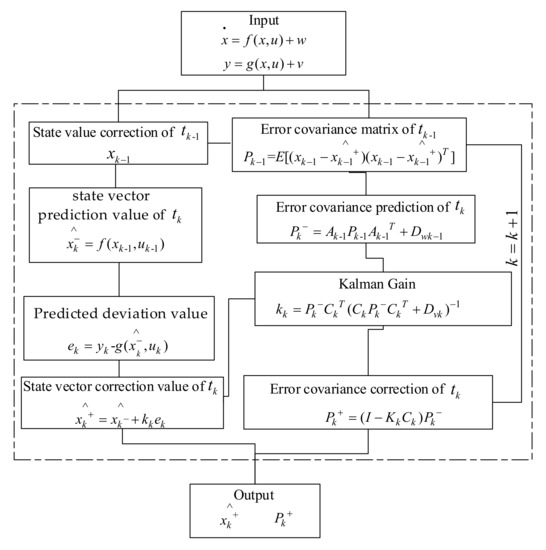
Figure 7.
Extend Kalman filter (EKF) estimation flowchart.
3.3. A Compound SOC Estimation Algorithm Based on Wavelet Transform
During the operation of a microgrid system, the fluctuation of current is relatively large, and therefore the EKF algorithm is chosen. In addition, the current and voltage of the battery are easily disturbed by the converter, so the wavelet denoising algorithm is applied for signal denoising. Therefore, the two algorithms are combined with developing respective advantages and a good performance optimization algorithm is obtained. It is relatively accurate to combine the algorithms in the engineering mentioned above. The proposed composite algorithm gives full play to the advantages of various algorithms, improves the SOC estimation accuracy, and meets the application of engineering. The flowchart of implementation of the proposed composite algorithm is shown in Figure 8.
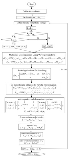
Figure 8.
The compound algorithm flowchart.
Step 1 Define the following variables, the minimum current , the standing time , the sampling time , the of , the of , the of , the SOC initial value , the Coulomb efficiency , and the current rate ;
Step 2 Establish the relationships between SOC and OCV, and between the Coulomb efficiency and the current rate;
Step 3 Establish a mathematical model of the lead carbon battery;
Step 4 If the batteries of BESS are in a static state ( and ), the value of OCV is equal to of , and the is obtained by Equation (4). If it is not in a static state, the value of is equal to of ;
Step 5 The of is estimated by the EKF based on wavelet denoising algorithm;
Step 6 The of is estimated through the Ah algorithm;
Step 7 In a group of batteries, select the minimum SOC value as the final output value.
4. Algorithm Validations and Analysis
4.1. Analysis and Verification of Experimental Data
In this study, the data of the first experiment in Section 2 is used to verify the accuracy and robustness. Because the initial SOC value is given, the real SOC is real-time calculated through the Ah integration method by the host computer.
- (1)
- Figure 9a shows the SOC result using the experimental data. The accuracy of the compound algorithm is very high, with the relative error within 0.6%.
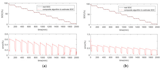 Figure 9. SOC estimation of experimental data. (a) Same ; (b) Different .
 - (2)
- Figure 9b displays the robustness of the algorithm. It is supposed that there is an initial deviation value ( of the compound algorithm is 0.5 while of the Ah algorithm is 1). The combined algorithm can correct the initial error quickly, and the final estimated relative error is within 0.6%.
4.2. Verification and Analysis of ESS Operation Data
The proposed composite algorithm was applied to two microgrid systems. The first microgrid system is a demonstration project located in Haining of Zhejiang Province. The ESS included lead carbon batteries and lead-acid batteries, and the capacity and the maximum output power was 1 MWh and 1.2 MW, respectively.
Table 4 displays the configuration parameters of the first microgrid system. Figure 10 shows the structure of the first microgrid system. The vertical view of the containerized ESS and its internal structure are shown in Figure 11 and Figure 12, respectively.
Table 4.
The parameters of the first microgrid system.
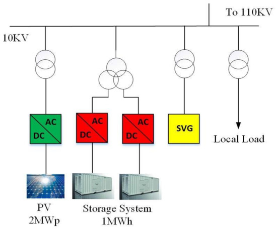
Figure 10.
Structure diagram of the first microgrid system.
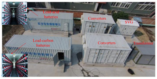
Figure 11.
The vertical view of the ESS.
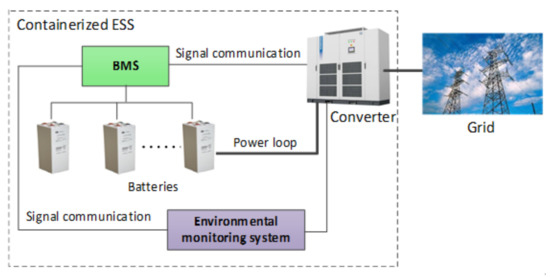
Figure 12.
Internal structure diagram of the container.
The ESS in the first microgrid system has two main functions. The first function is to achieve the best economy by cutting peak and filling valley of the time-of-use (TOU) electricity price; the second function is to improve the stability by smoothing PV power fluctuation when PV is connected to the grid [3].
In order to test the accuracy of the composite method, the ESS operational data of 24 h is selected for analysis. In this study, three methods (the EKF, the EKF based on wavelet transform, and the composite algorithm) are used to estimate SOC. Figure 13 and Figure 14 show the results of the SOC estimation.
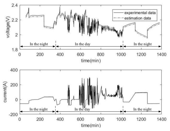
Figure 13.
Single battery operation data and its model simulation.
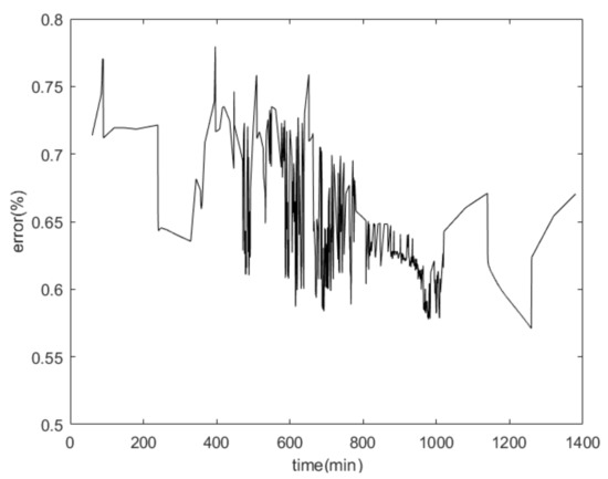
Figure 14.
Battery model simulation error result.
There are three curves shown in Figure 13. The experimental data curve is the voltage curve of a single battery of the BESS. The estimation data curve is the voltage curve simulated by the battery model mentioned above. The current curve is a group of lead carbon batteries of the ESS. The operation conditions of the following TOU price are visible at night and smoothing the PV power fluctuation are visible during the day. As shown in Figure 14, the relative error of simulation is within 0.8%.
According to practical experience and the above discussion, the signal denoising of the first demonstration project of microgrid is based on Haar features, with the decomposition layer being chosen as four layers. Table 5 shows the threshold values at each level of the sampled voltage and current signals. Figure 15 displays the original signals and the denoised signals. Noise interference in current and voltage signals is eliminated effectively through this denoised algorithm.
Table 5.
Threshold values at each level.
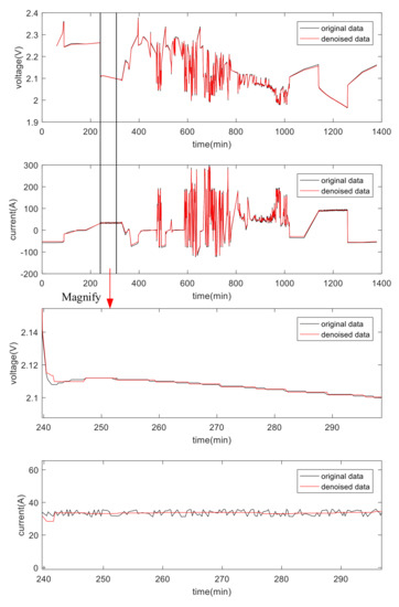
Figure 15.
Denoising approach.
As shown in Figure 16, we can see the results of the comparison and error analysis of different algorithms for estimating SOC. It can be observed that the three methods effectively track the real SOC, and the estimated accuracies of these three methods are 0.9%, 0.6%, and 0.5%, respectively. The composite algorithm is the most accurate in the entire estimation process.
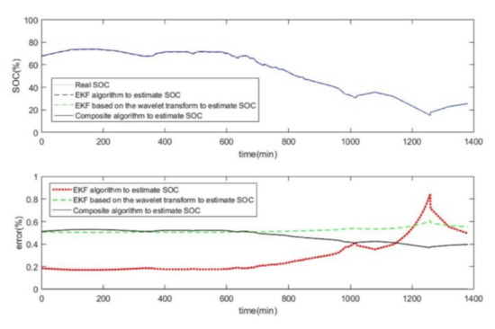
Figure 16.
SOC estimation results.
The second microgrid system is also a demonstration project located in Xining City, Qinghai Province, China. The configuration parameters of the second microgrid system are listed in Table 6.
Table 6.
The parameters of the second microgrid system.
The structure of the microgrid is shown in Figure 17, and the vertical view of it is shown in Figure 18. The internal structure of the containerized ESS is the same as the one shown in Figure 12.
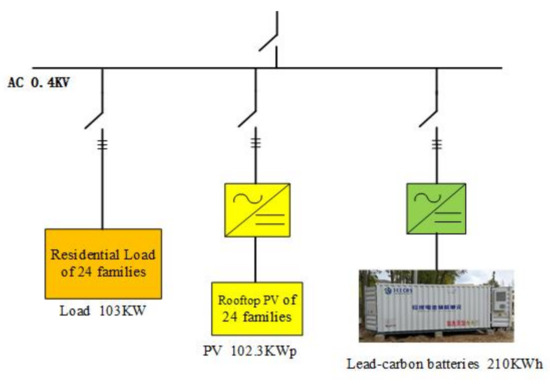
Figure 17.
Structure diagram of the second microgrid system.
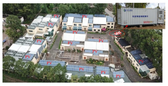
Figure 18.
The vertical view of the microgrid system.
The ESS has two main functions in this microgrid system, increasing the penetration of renewable energy when connected to the grid, and supporting load normal operation when off the grid, therefore, the microgrid system can operate independently.
The penetration of renewable energy refers to the proportion of renewable energy in load power consumption.
where P is penetration of renewable energy.
Increasing penetration is beneficial, improving the economy of the microgrid system and reducing the negative impact of PV and load power fluctuations on the stability of the grid. However, the excessive pursuit of penetration can lead to unreasonable regulation of PV and load, which reduces the economy of the system. Therefore, it is essential to obtain the optimal control strategy with consideration of cost and penetration. The control strategy of the microgrid is mainly carried out in the daytime. At night, the ESS is charged because of the low valley electricity prices in order to meet the power demand for load when the peak electric price is executed the next morning.
As shown in Figure 19, due to the existence of the ESS, the grid-connected power of microgrid is small, and the penetration of renewable energy is improved. As shown in Figure 20, the load power consumption in one day is 462.6 kWh, the PV generating capacity in one day is 369.5 kWh, and the PV power consumption connected to the grid in one day is 70 kWh. According to the definition of penetration of renewable energy, the penetration is 64.7%. The data of the flat segment in the middle of Figure 20 should be lost, which is not important, but the final accumulation data of the day is considered.
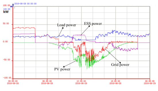
Figure 19.
Power curves of a microgrid connected to the grid.
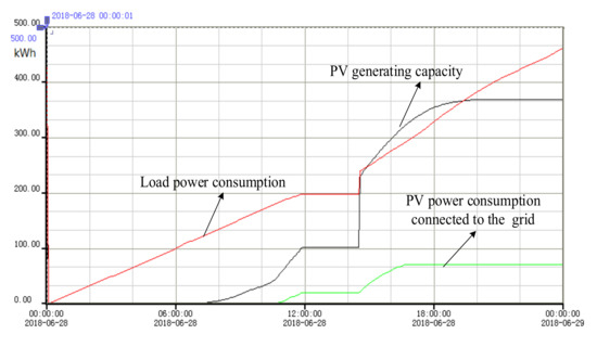
Figure 20.
Electricity quantity curves of a microgrid connected to the grid.
In order to verify the effectiveness of the proposed composite algorithm, 24 h of the ESS operation data is used for the analysis similar to the first microgrid system. The estimation results are shown in Figure 21, Figure 22, Figure 23 and Figure 24.
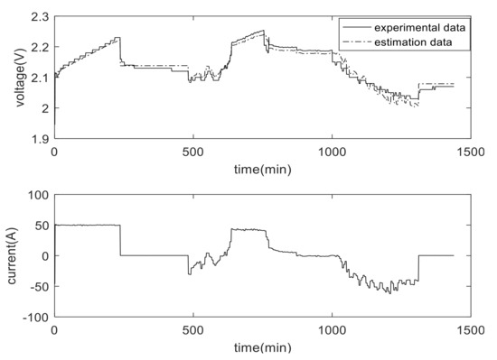
Figure 21.
Single battery operation data and its model simulation.
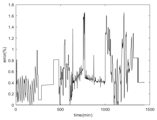
Figure 22.
Battery model simulation error result.
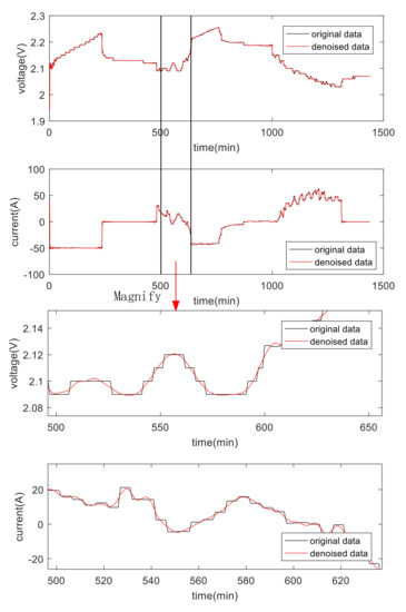
Figure 23.
Denoising approach.
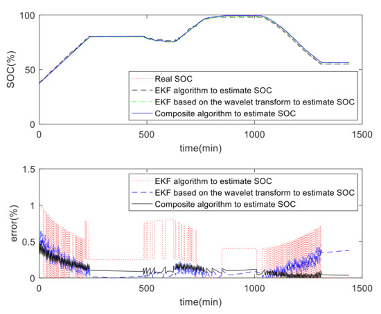
Figure 24.
SOC estimation results.
In Figure 21, there are two voltage curves of experimental data and estimation data and a current data curve of one battery in the ESS. The operation conditions of increasing the permeability of renewable energy can be seen. In order to improve energy permeability, the ESS power is used first, which bears the power difference between PV and load. It is charged when the PV power is large and discharged when the PV power cannot meet the load demand. The data of the ESS power is intercepted to analyze the operation condition of the batteries and the simulation results of the battery model are analyzed. The relative error of simulation is within 1.8%, as shown in Figure 22.
The denoising signal of battery in the microgrid is based on dmey (a common wavelet base for decomposition), with the decomposition layer divided into four layers. Table 7 demonstrates the threshold values of signals at each level and Figure 23 demonstrates the original signals and the denoised signals. The noise interference in the signals is eliminated effectively through this denoised algorithm.
Table 7.
Threshold values at each level.
As can be seen in Figure 24, the three methods effectively track the real SOC, and the estimated accuracies are 1%, 0.6%, and 0.5%, respectively.
When the grid is cut off, the microgrid operates independently. At this time, as the only voltage source in the microgrid, the ESS needs to support the bus voltage stability of the microgrid to ensure the normal operation of the important load.
In the case of power failure and other faults in the power grid, the microgrid is disconnected from the external power grid. In order to guarantee the reliable power supply of the important load under the off-grid condition, the control strategy is mainly as follows: Because the energy storage converter is the only voltage source in the microgrid, it is essential to support the voltage stability of the microgrid bus to ensure the normal power consumption of the system load. It can actively regulate the PV and load power in this system, so as to meet the power and capacity requirements of the ESS and increase the off-grid operation time. Figure 25 demonstrates the power waveform of the microgrid running off the grid, during which period the grid-connected power, as the judgment condition of off-grid operation, is maintained at 0, with the off-grid operation time of the microgrid reaching around 8 h. The power of the load is completely provided by PV power and ESS power.
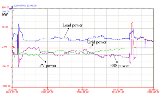
Figure 25.
Power curves of a microgrid off the grid.
In Figure 26, there are two voltage curves of experimental data and estimation data and a current data curve of one battery in the ESS. The operation conditions that support normal operation of the important load can be seen. The data of the ESS power is intercepted to analyze the operation condition of the batteries. The microgrid system operates independently and supports normal load operation when off the grid. The simulation results of the battery model are analyzed. As shown in Figure 27, the relative error of the SOC estimation is within 0.8%.
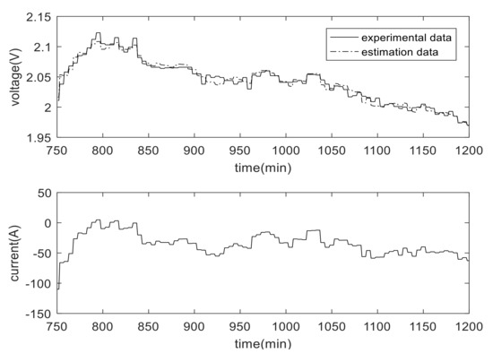
Figure 26.
Single battery operation data and its model simulation.
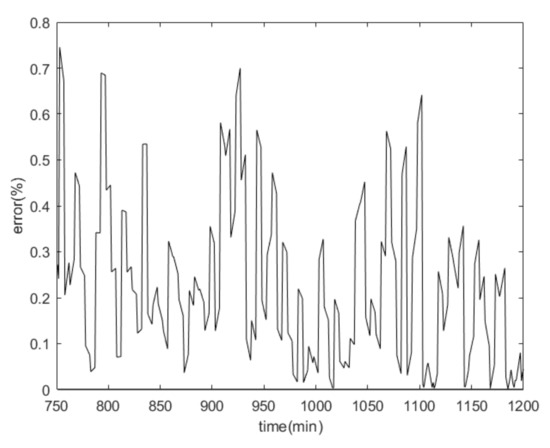
Figure 27.
Battery model simulation error result.
The denoising signal of the battery in the microgrid is based on dmey (a common wavelet base for decomposition), with the decomposition layer divided into four layers. Table 8 summarizes the threshold values of the current and voltage signals at each level. Figure 28 shows the original signals and the denoised voltage and current signals.
Table 8.
Threshold values at each level.
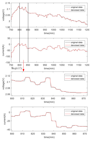
Figure 28.
Denoising approach.
Figure 29 shows the results of the comparison and relative error analysis of different algorithms for estimating SOC. We seen that the three methods effectively track the real SOC, with the estimated accuracy of these three methods maintaining 1.1%, 1%, and 0.5%, respectively. The accuracy of the composite algorithm is the best in the whole estimation process.
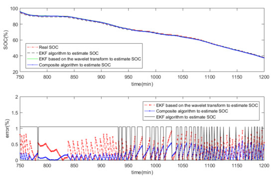
Figure 29.
SOC estimation results.
5. Conclusions
On the basis of a series of data analysis, the proposed composite estimation algorithm is the best of the tested methods to estimate the SOC of lead carbon batteries. The experimental results demonstrate that the compound estimation algorithm with a relative error of within 0.5% is obviously superior to the other algorithms.
The proposed composite method is suitable for applications in the field of an ESSs in microgrid systems. Its advantages are as follows:
- In this study, three algorithms were used to estimate SOC. The EKF algorithm estimates the SOC accurately, but it does not eliminate system noise, while the EKF based on the wavelet transform algorithm estimates the SOC accurately by eliminating system noise. The above two algorithms are based on accurate identification of the parameters of the battery model. If the parameters are not identified accurately in the process of iterative correction, the precision of SOC estimation is significantly affected. The proposed composite algorithm, in this study, has many advantages. The OCV-SOC method is used to determine the initial value of SOC. There is a simple correction link when the initial value is determined. Then, in the process of denoising and EKF estimation, the SOC estimation is combined with the Ah method. In this way, one step of estimation is carried out without relying on the battery model, and the precision of estimation is increased.
- The composite algorithm suppresses the system noise and satisfies the needs of engineering applications in the ESS of the microgrid system.
- Compared with other methods, it is relatively accurate in the frequent high-current charge and discharge conditions, especially the complex and changeable operating conditions.
- This research demonstrates that the proposed composite method has the characteristics of robustness.
- The battery model used, in this study, does not consider the influence of temperature, and the accuracy of estimation needs to be improved.
Author Contributions
Y.C. and Z.Y. conceived the main idea and performed the tests, data analysis and wrote the manuscript. Y.W. gave suggestions and data processing. All authors have read and agreed to the published version of the manuscript.
Funding
This research was funded by [the Qinghai Major Science and Technology program] grant number [2019-GX-A] and [the K.C.Wong Education Foundation] grant number [GJTD-2018-05].
Conflicts of Interest
The authors declare no conflict of interest.
References
- Grillo, S.; Marinelli, M.; Massucco, S.; Silvestro, F. Optimal management strategy of a battery-based storage system to improve renewable energy integration in distribution networks. IEEE Trans. Smart Grid 2012, 3, 950–958. [Google Scholar] [CrossRef]
- Jiang, Q.; Gong, Y.; Wang, H. A battery energy storage system dual layer control strategy for mitigating wind farm fluctuations. IEEE Trans. Power Syst. 2013, 28, 3263–3273. [Google Scholar] [CrossRef]
- Guo, L.D.; Lei, M.Y.; Yang, Z.L.; Wang, Y.B.; Xu, H.H.; Chen, Y.Y. Research on control strategy of the energy storage system for photovoltaic and storage combined system. In Proceedings of the IECON 2017-43rd Annual Conference of the IEEE Industrial Electronics Society, Beijing, China, 29 October–1 November 2017; pp. 2813–2817. [Google Scholar]
- Dan, W.; Fen, T.; Dragicevic, T.; Vasquez, J.C.; Guerrero, J.M. Autonomous active power control for islanded AC microgrids with photovoltaic generation and energy storage system. IEEE Trans. Energy Convers. 2014, 29, 882–892. [Google Scholar]
- Kim, J.Y.; Jeon, J.H.; Kim, S.K.; Cho, C.; Park, J.H.; Kim, H.M.; Nam, K.Y. Cooperative control strategy of energy storage system and microsources for stabilizing the microgrid during islanded operation. IEEE Trans. Power Electron. 2010, 25, 3037–3048. [Google Scholar]
- Sebastián, R. Application of a battery energy storage for frequency regulation and peak shaving in a wind diesel power system. IET Gener. Transm. Dist. 2016, 10, 764–770. [Google Scholar] [CrossRef]
- Anderson, J.L.; Frankhouser, J. Advanced lead carbon batteries for partial state of charge operation in stationary applications. In Proceedings of the 2015 IEEE International Telecommunications Energy Conference (INTELEC), Osaka, Japan, 18–22 October 2015; IEEE: Piscataway, NJ, USA, 2016. [Google Scholar]
- Yang, Z.; Zhang, J.; Kintner-Meyer, M.C.; Lu, X.; Choi, D.; Lemmon, J.P.; Liu, J. Electrochemical energy storage for green grid. Chem. Rev. 2011, 111, 3577–3613. [Google Scholar] [CrossRef]
- Tong, P.; Zhao, R.; Zhang, R.; Yi, F.; Shi, G.; Li, A.; Chen, H. Characterization of lead (II)-containing activated carbon and its excellent performance of extending lead-acid battery cycle life for high-rate partial-state-of-charge operation. J. Power Sources 2015, 286, 91–102. [Google Scholar] [CrossRef]
- Xiang, J.; Ding, P.; Zhang, H.; Wu, X.; Chen, J.; Yang, Y. Beneficial effects of activated carbon additives on the performance of negative lead-acid battery electrode for high-rate partial-state-of-charge operation. J. Power Sources 2013, 241, 150–158. [Google Scholar] [CrossRef]
- Lawder, M.T.; Suthar, B.; Northrop, P.W.; De, S.; Hoff, C.M.; Leitermann, O.; Crow, M.L. Battery Energy Storage System (BESS) and Battery Management System (BMS) for Grid-Scale Applications. Proc. IEEE 2014, 102, 1014–1030. [Google Scholar] [CrossRef]
- Elsayed, A.T.; Lashway, C.R.; Mohammed, O.A. Advanced Battery Management and Diagnostic System for Smart Grid Infrastructure. IEEE Trans. Smart Grid 2016, 7, 897–905. [Google Scholar]
- Dang, X.; Yan, L.; Xu, K.; Wu, X.; Jiang, H.; Sun, H. Open-Circuit Voltage-Based State of Charge Estimation of Lithium-ion Battery Using Dual Neural Network Fusion Battery Model. Electrochim. Acta 2015, 188, 356–366. [Google Scholar] [CrossRef]
- Yang, N.; Zhang, X.; Li, G. State of charge estimation for pulse discharge of a LiFePO4 battery by a revised Ah counting. Electrochim. Acta 2015, 151, 63–71. [Google Scholar] [CrossRef]
- Chen, Z.; Fu, Y.; Mi, C.C. State of Charge Estimation of Lithium-Ion Batteries in Electric Drive Vehicles Using Extended Kalman Filtering. Veh. Technol. 2013, 62, 1020–1030. [Google Scholar] [CrossRef]
- Chen, J.; Ouyang, Q.; Xu, C.; Su, H. Neural Network-Based State of Charge Observer Design for Lithium-Ion Batteries. IEEE Trans. Control Syst. Technol. 2017, 26, 313–320. [Google Scholar] [CrossRef]
- Anton, J.C.A.; Nieto, P.J.G.; Viejo, C.B.; Vilán, J.A.V. Support Vector Machines Used to Estimate the Battery State of Charge. IEEE Trans. Power Electron. 2013, 28, 5919–5926. [Google Scholar] [CrossRef]
- Plett, G.L. Extended Kalman filtering for battery management systems of LiPB-based HEV battery packs. J. Power Sources 2004, 134, 262–276. [Google Scholar] [CrossRef]
- Chen, M.; Rincon-Mora, G.A. Accurate electrical battery model capable of predicting runtime and I-V performance. IEEE Trans. Energy Convers. 2006, 21, 504–511. [Google Scholar] [CrossRef]
- Chen, Y.; Yang, Z.; Guo, L.; Huang, X.; Wang, Y. A composite estimation method for state of charge of batteries in a power station engineering. In Proceedings of the 2017 IEEE Conference on Energy Internet & Energy System, Beijing, China, 26–28 November 2017; pp. 1–6. [Google Scholar]
- Chen, Y.; Yang, Z.; Wang, Y.; Guo, L.; Huang, X. State of charge estimation of lead-carbon batteries in actual engineering. In Proceedings of the 2017 20th International Conference on Electrical Machines & Systems, Sydney, Australia, 11–14 August 2017; pp. 1–6. [Google Scholar]
- Boubchir, L.; Boashash, B. Wavelet denoising based on the MAP estimation using the BKF with application to images and EEG signals. IEEE Trans. Signal Process. 2013, 61, 1880–1894. [Google Scholar] [CrossRef]
- Hu, X.S.; Li, S.B.; Li, H.; Peng, F.C. Robustness analysis of State-of-Charge estimation methods for two types of Li-ion batteries. J. Power Sources 2012, 217, 209–219. [Google Scholar] [CrossRef]
- Farahani, M.A.; Wylie, M.T.V.; Guerra, E.C.; Colpitts, B.G. Reduction in the number of averages required in BOTDA sensors using wavelet denoising techniques. J. Lightw. Technol. 2012, 30, 1134–1142. [Google Scholar] [CrossRef]
- Ismail, B.; Khan, A. Image De-noising with a New Threshold Value Using Wavelets. J. Data Sci. 2012, 10, 259–270. [Google Scholar]
- Zafar, S.; Zhang, Y.Q.; Jabbari, B. Multiscale video representation using multiresolution motion compensation and wavelet decomposition. IEEE J. Sel. Areas Commun. 2002, 11, 24–35. [Google Scholar] [CrossRef]
- Dong, W.; Ding, H. Full Frequency De-noising Method Based on Wavelet Decomposition and Noise-type Detection. Neurocomputing 2016, 214, 902–909. [Google Scholar] [CrossRef]
- Baykal-Gursoy, M. Forecasting: State-Space Models and Kalman Filter Estimation; ResearchGate: Berlin, Germany, 2011. [Google Scholar]
- Sun, F.; Xiong, R. A novel dual-scale cell state-of-charge estimation approach for series-connected battery pack used in electric vehicles. J. Power Sources 2015, 274, 582–594. [Google Scholar] [CrossRef]
- Paschero, M.; Storti, G.L.; Rizzi, A.; Mascioli, F.M.F.; Rizzoni, G. A Novel Mechanical Analogy-Based Battery Model for SoC Estimation Using a Multicell EKF. IEEE Trans. Sustain. Energy 2016, 7, 1695–1702. [Google Scholar] [CrossRef]
- He, Z.; Gao, M.; Xu, J. EKF-Ah Based State of Charge Online Estimation for Lithium-ion Power Battery. In Proceedings of the 2009 International Conference on Computational Intelligence and Security, Beijing, China, 11–14 December 2009; Volume 1, pp. 142–145. [Google Scholar]
- Kim, J.; Cho, B.H. State-of-Charge Estimation and State-of-Health Prediction of a Li-Ion Degraded Battery Based on an EKF Combined with a Per-Unit System. IEEE Trans. Veh. Technol. 2011, 60, 4249–4260. [Google Scholar] [CrossRef]


© 2019 by the authors. Licensee MDPI, Basel, Switzerland. This article is an open access article distributed under the terms and conditions of the Creative Commons Attribution (CC BY) license (http://creativecommons.org/licenses/by/4.0/).