Quantitative Analysis of the Sensitivity of UHF Sensor Positions on a 420 kV Power Transformer Based on Electromagnetic Simulation


Abstract
1. Introduction
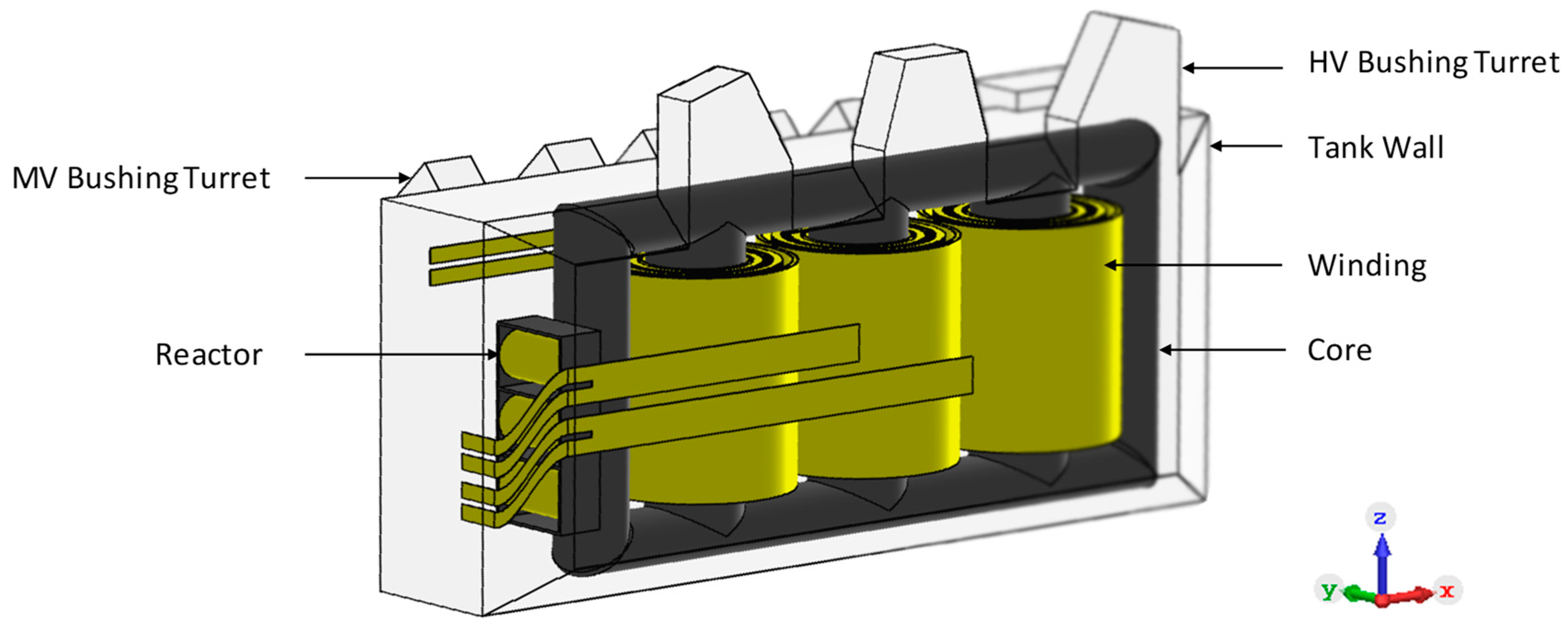
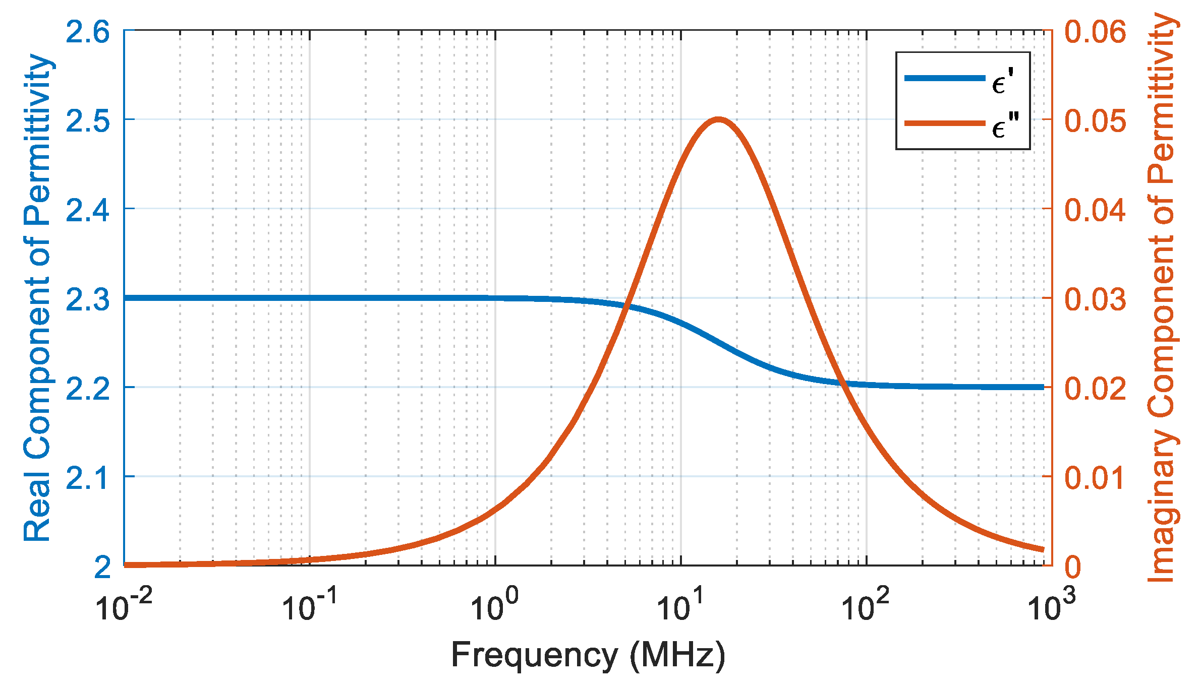
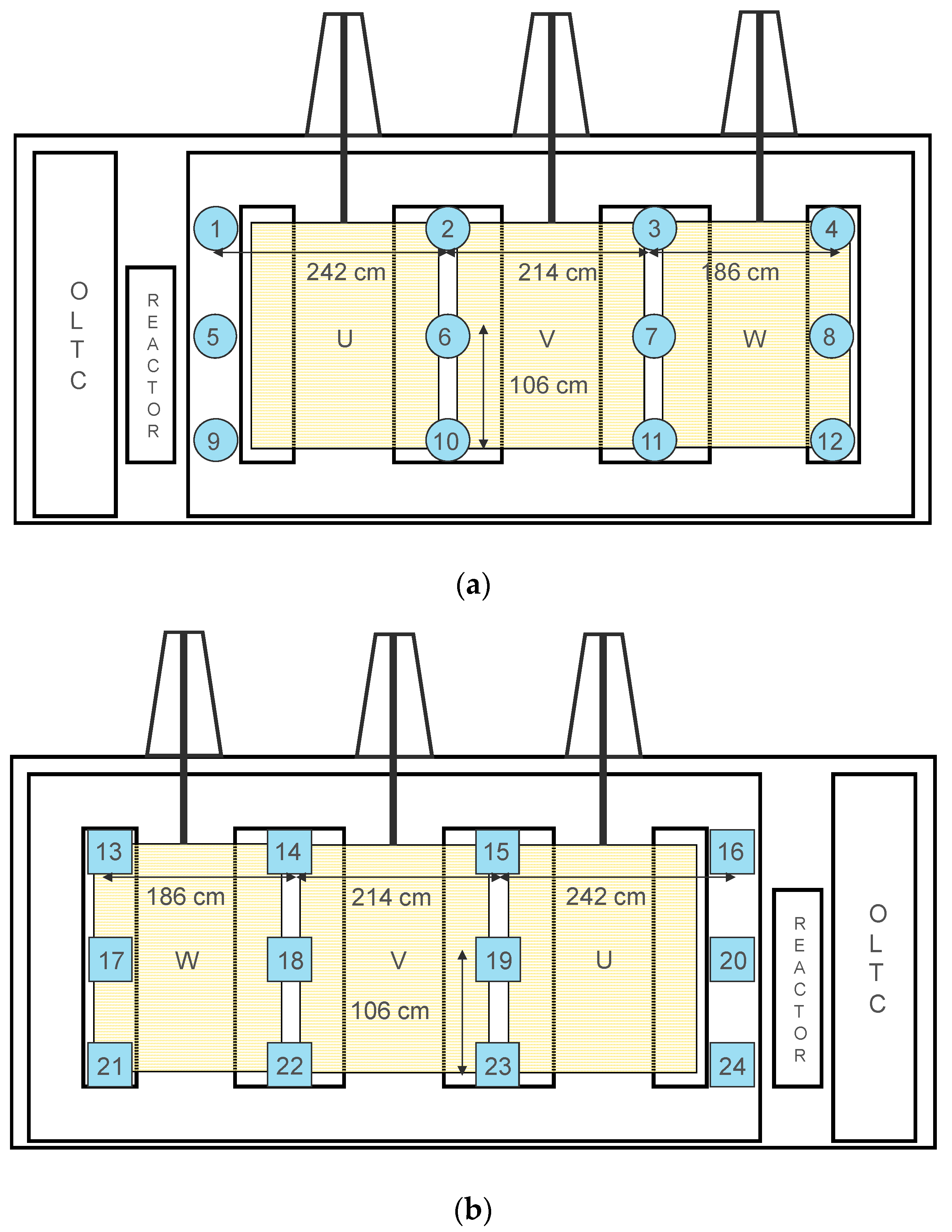
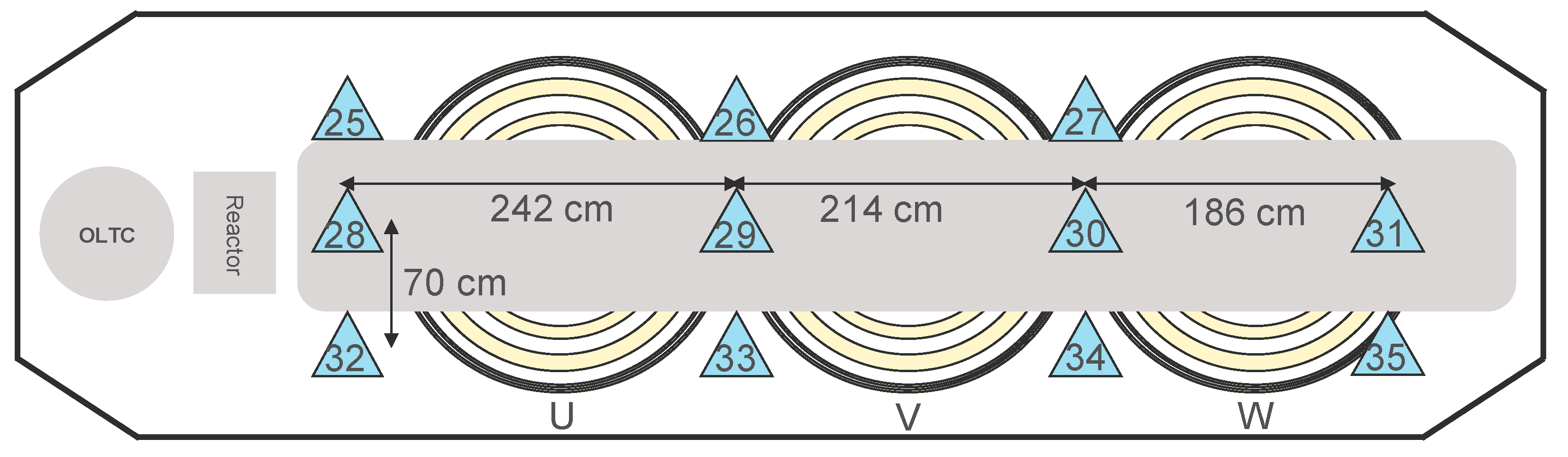
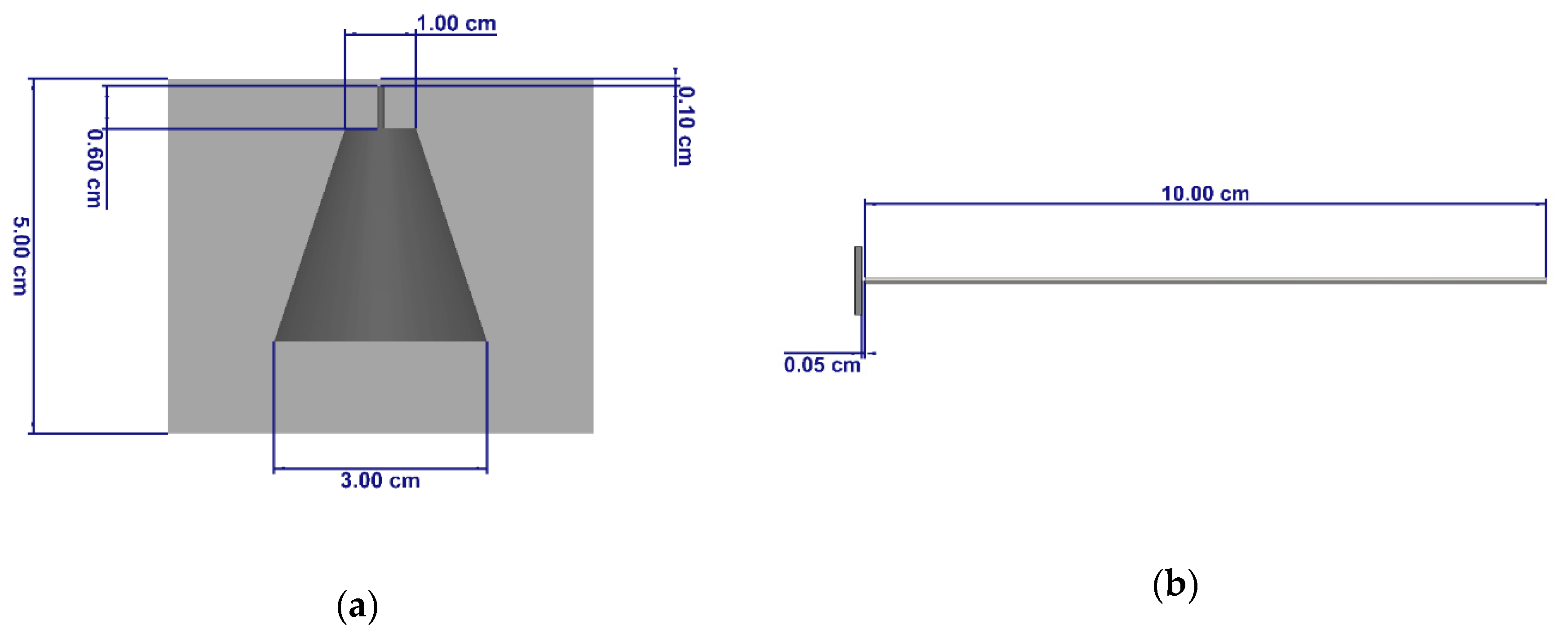
2. Simulation Setup
3. Results
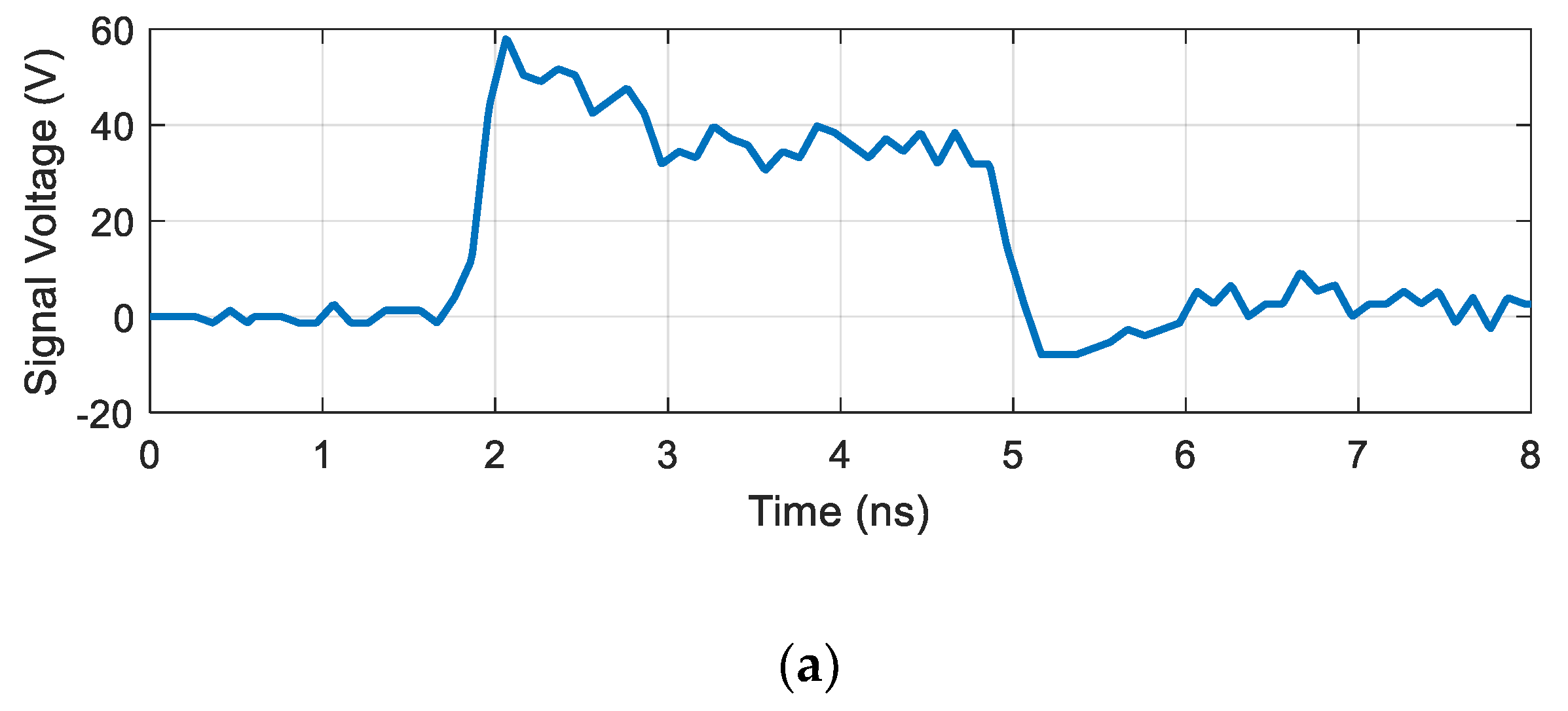
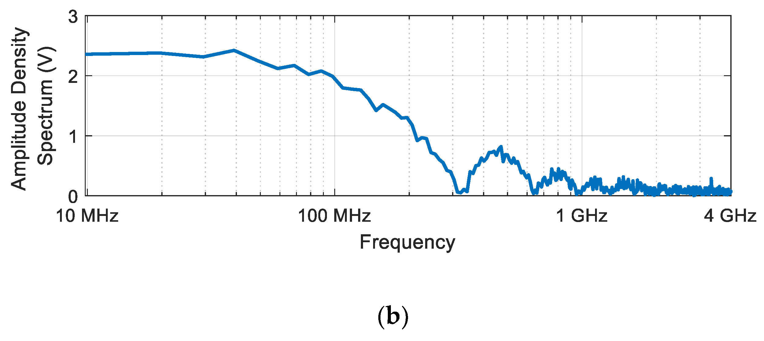
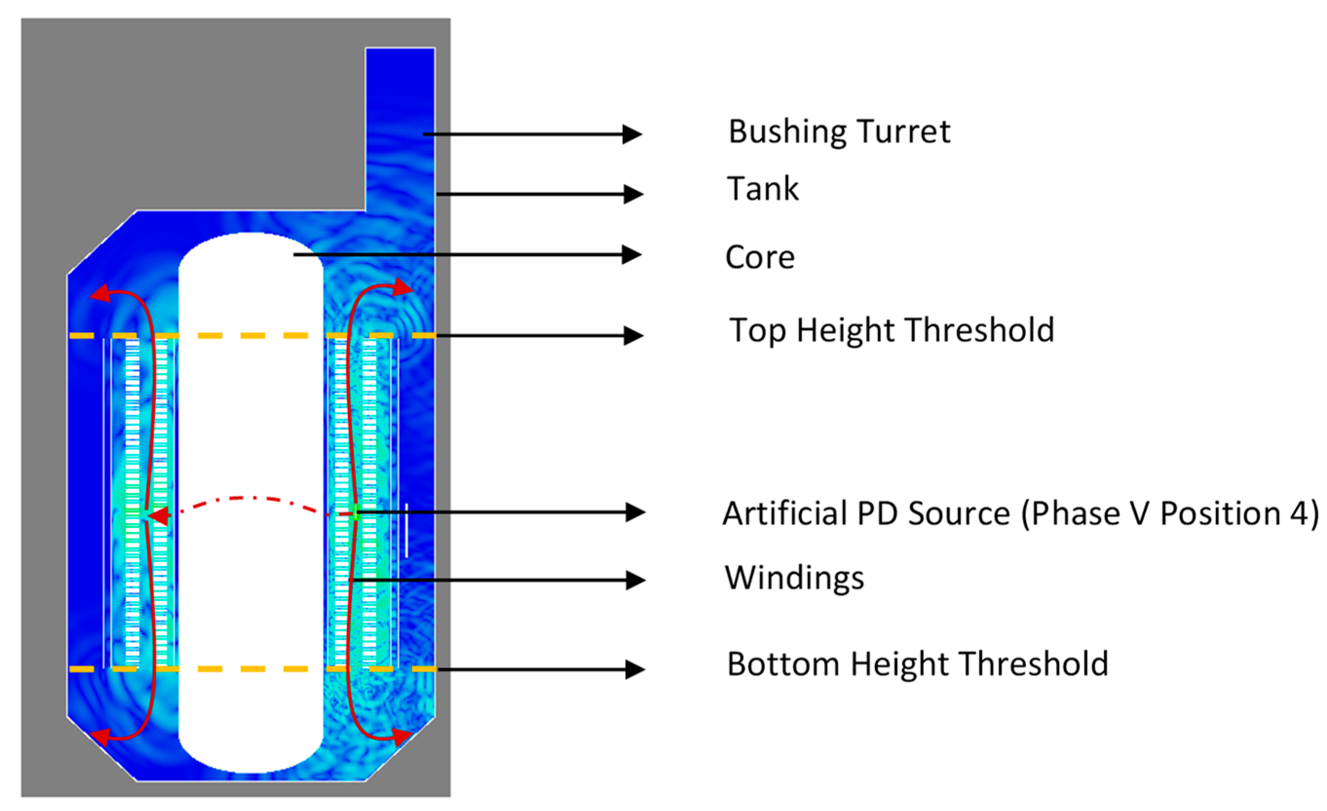
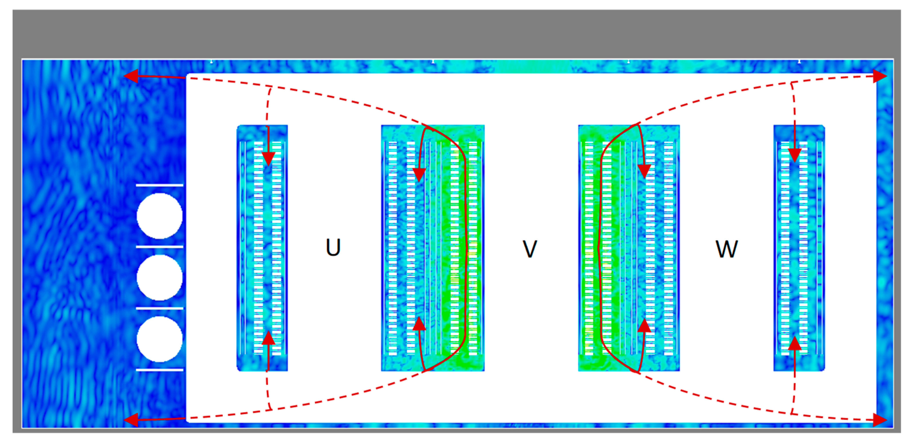
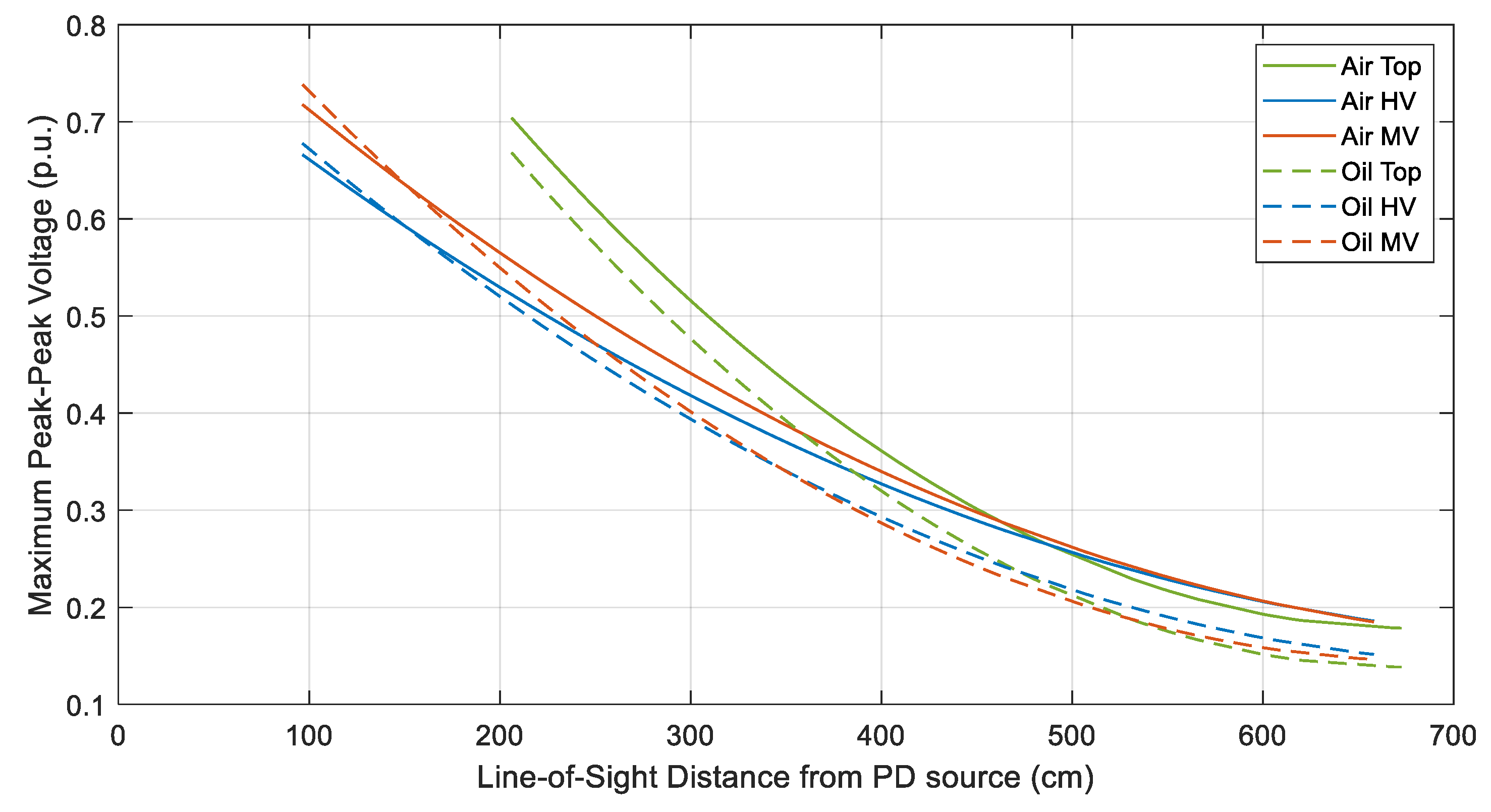
3.1. Signal Propagation and Attenuation Characteristics
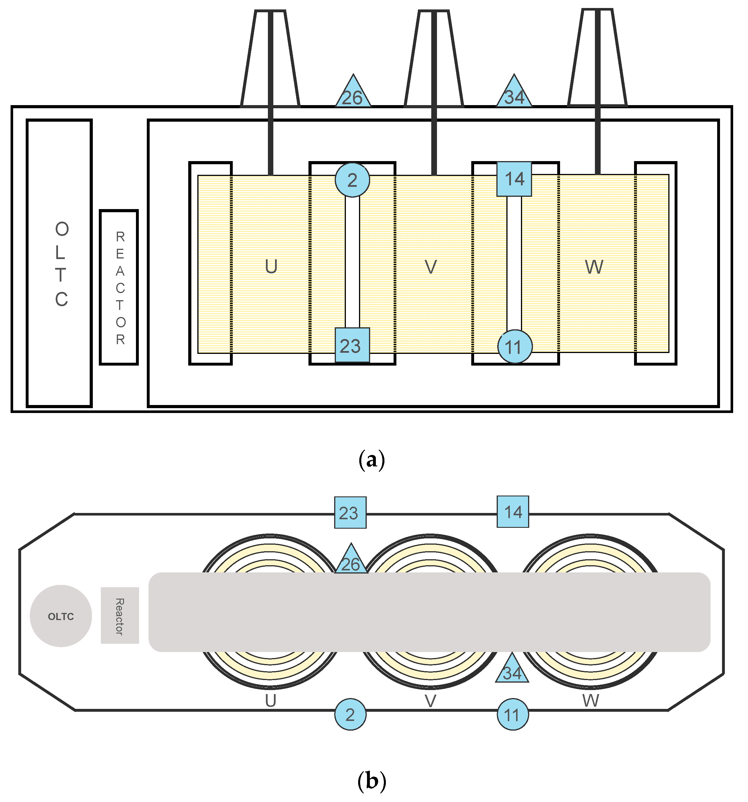
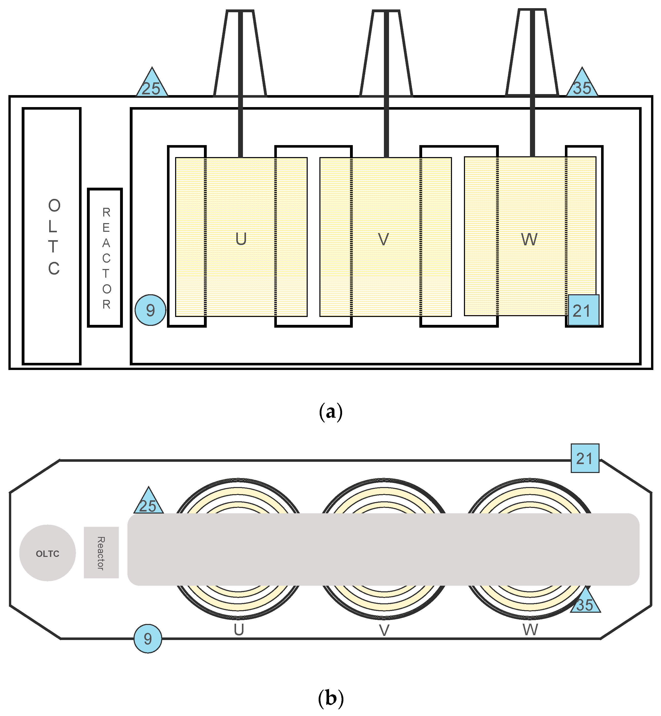
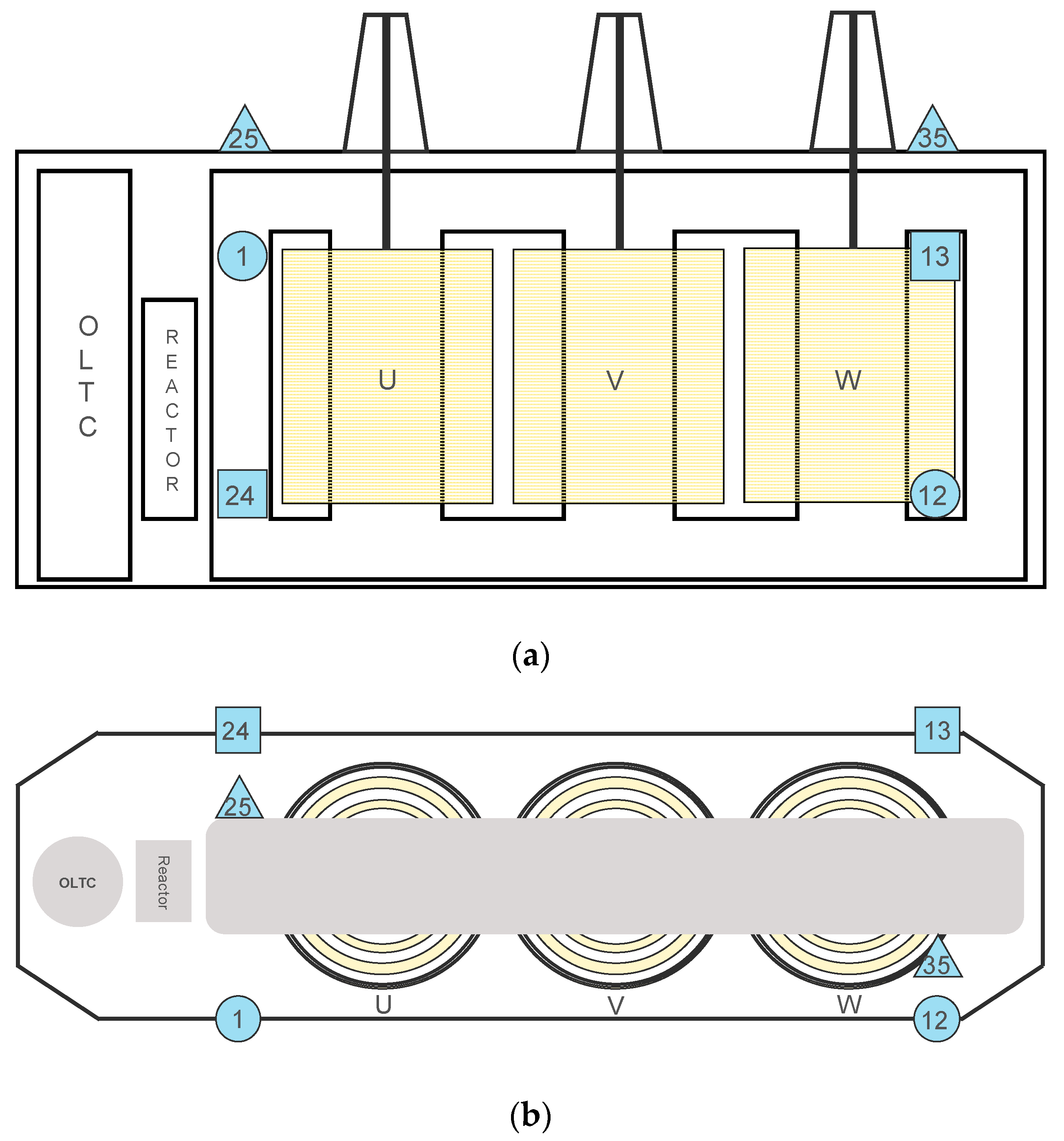
3.2. Sensitivity Analysis of Different Sensor Positions
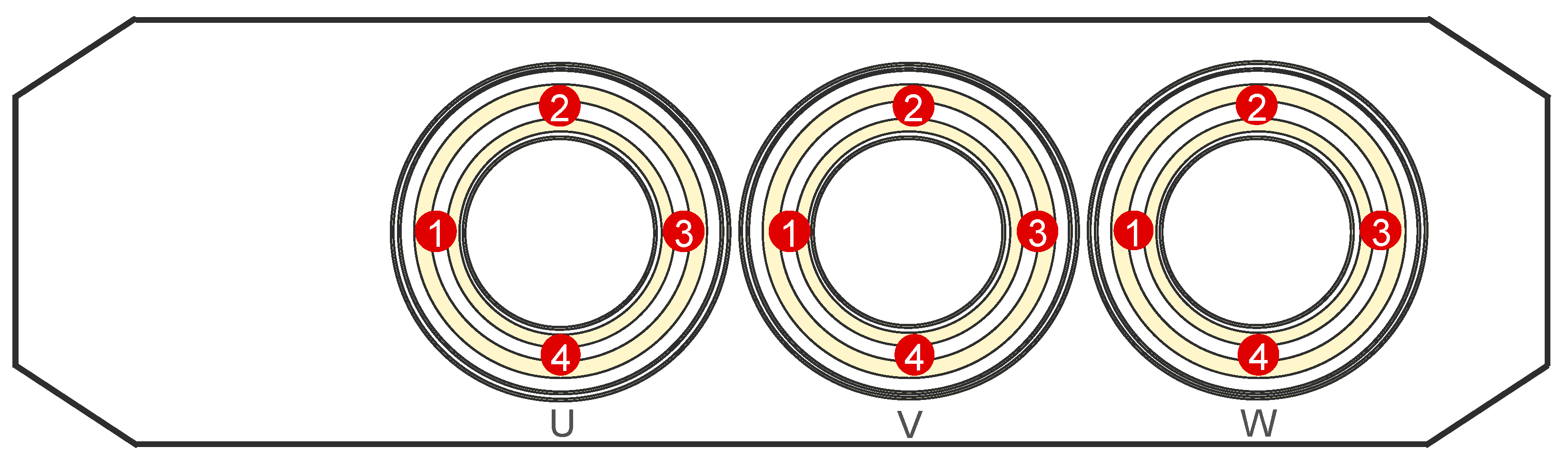
3.2.1. HV and MV/LV Sensors
3.2.2. Top Sensors
3.2.3. Most Sensitive Sensor Positions
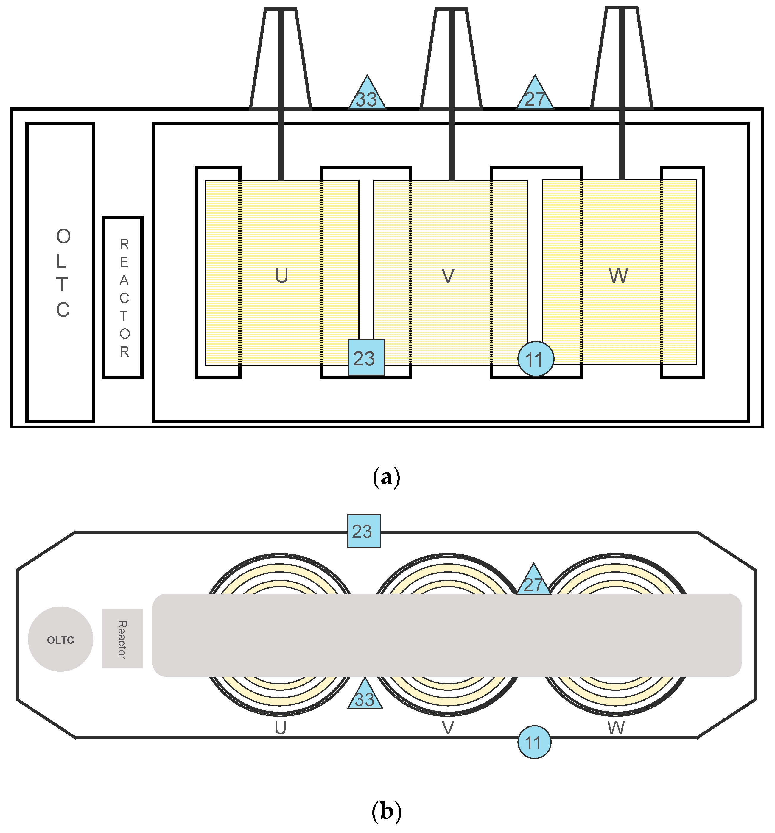
3.3. Proposals for Optimal Sensor Placement for PD Source Localization
3.3.1. Using Most Sensitive Sensor Positions
3.3.2. Maximizing Distance from High Field Stress Regions
4. Conclusions
5. Outlook
Author Contributions
Funding
Conflicts of Interest
References
- International Electrotechnical Commission. IEC 62478 High Voltage Test Techniques—Measurement of Partial Discharges by Electromagnetic and Acoustic Methods; IEC: Geneva, Switzerland, 2016; ISBN 978-2-83-223560-7. [Google Scholar]
- Chai, H.; Phung, B.T.; Mitchell, S. Application of UHF Sensors in Power System Equipment for Partial Discharge Detection: A Review. Sensors 2019, 19, 1029. [Google Scholar] [CrossRef] [PubMed]
- Tenbohlen, S.; Beltle, M.; Siegel, M. PD monitoring of power transformers by UHF sensors. In Proceedings of the 2017 International Symposium on Electrical Insulating Materials (ISEIM), Toyohashi, Japan, 11–15 September 2017; pp. 303–306, ISBN 978-4-88-686099-6. [Google Scholar]
- Dukanac, D. Application of UHF method for partial discharge source location in power transformers. IEEE Trans. Dielect. Electr. Insul. 2018, 25, 2266–2278. [Google Scholar] [CrossRef]
- Romano, P.; Imburgia, A.; Ala, G. Partial Discharge Detection Using a Spherical Electromagnetic Sensor. Sensors 2019, 19, 1014. [Google Scholar] [CrossRef] [PubMed]
- Nobrega, L.A.M.M.; Xavier, G.V.R.; Aquino, M.V.D.; Serres, A.J.R.; Albuquerque, C.C.R.; Costa, E.G. Design and Development of a Bio-Inspired UHF Sensor for Partial Discharge Detection in Power Transformers. Sensors 2019, 19, 653. [Google Scholar] [CrossRef] [PubMed]
- Zachariades, C.; Shuttleworth, R.; Giussani, R. A Dual-Slot Barrier Sensor for Partial Discharge Detection in Gas-Insulated Equipment. IEEE Sensors J. 2019, 1. [Google Scholar] [CrossRef]
- Li, J.; Han, X.; Liu, Z.; Yao, X. A Novel GIS Partial Discharge Detection Sensor With Integrated Optical and UHF Methods. IEEE Trans. Power Deliv. 2018, 33, 2047–2049. [Google Scholar] [CrossRef]
- CIGRÉ. Guidelines for Partial Discharge Detection Using Conventional (IEC 60270) and Unconventional Methods; CIGRÉ: Paris, France, 2016; ISBN 978-2-85-873365-1. [Google Scholar]
- Nobrega, L.; Costa, E.; Serres, A.; Xavier, G.; Aquino, M. UHF Partial Discharge Location in PowerTransformers via Solution of the MaxwellEquations in a Computational Environment. Sensors 2019, 19, 3435. [Google Scholar] [CrossRef] [PubMed]
- Xue, N.; Yang, J.; Shen, D.; Xu, P.; Yang, K.; Zhuo, Z.; Zhang, L.; Zhang, J. The Location of Partial Discharge Sources Inside Power Transformers Based on TDOA Database with UHF Sensors. IEEE Access 2019, 7, 146732–146744. [Google Scholar] [CrossRef]
- Siegel, M.; Coenen, S.; Beltle, M.; Tenbohlen, S.; Weber, M.; Fehlmann, P.; Hoek, S.M.; Kempf, U.; Schwarz, R.; Linn, T.; et al. Calibration Proposal for UHF Partial Discharge Measurements at Power Transformers. Energies 2019, 12, 3058. [Google Scholar] [CrossRef]
- Siegel, M.; Tenbohlen, S. Calibration of UHF Partial Discharge Measurement for Power Transformers and a Comparison to the Calibration of Electrical PD Measurement. In Proceedings of the IEEE Electrical Insulation Conference, Montréal, QC, Canada, 19–22 June 2016. [Google Scholar]
- International Electrotechnical Commission. IEC 60270 High-Voltage Test Techniques: Partial Discharge Measurements; IEC: Geneva, Switzerland, 2000. [Google Scholar]
- Mirzaei, H.R.; Akbari, A.; Zanjani, M.; Miralikhani, K.; Gockenbach, E.; Borsi, H. Investigating suitable positions in power transformers for installing UHF antennas for partial discharge localization. In Proceedings of the 2012 IEEE International Conference on Condition Monitoring and Diagnosis (CMD), Bali, Indonesia, 23–27 September 2012; pp. 625–628, ISBN 978-1-46-731020-8. [Google Scholar]
- Siegel, M.; Beltle, M.; Tenbohlen, S.; Coenen, S. Application of UHF sensors for PD measurement at power transformers. IEEE Trans. Dielect. Electr. Insul. 2017, 24, 331–339. [Google Scholar] [CrossRef]
- Beura, C.P.; Beltle, M.; Tenbohlen, S. Positioning of UHF PD Sensors on Power Transformers Based on the Attenuation of UHF Signals. IEEE Trans. Power Delivery 2019, 34, 1520–1529. [Google Scholar] [CrossRef]
- Giglia, G.; Ala, G.; Castiglia, V.; Imburgia, A.; Miceli, R.; Rizzo, G.; Romano, P.; Schettino, G.; Viola, F. Electromagnetic Full-Wave Simulation of Partial Discharge Detection in High Voltage AC Cables. In Proceedings of the 2019 IEEE 5th International forum on Research and Technology for Society and Industry (RTSI), Florence, Italy, 9–12 September 2019; pp. 166–171, ISBN 978-1-72-813815-2. [Google Scholar]
- Beura, C.P.; Beltle, M.; Tenbohlen, S. Attenuation of UHF Signals in a 420 kV Power Transformer Based on Experiments and Simulation. In Proceedings of the 21st International Symposium on High Voltage Engineering; Németh, B., Ed.; Springer International Publishing: Cham, Germany, 2020; pp. 1276–1285. [Google Scholar]
- Umemoto, T.; Tenbohlen, S. Novel Simulation Technique of Electromagnetic Wave Propagation in the Ultra High Frequency Range within Power Transformers. Sensors 2018, 18, 4236. [Google Scholar] [CrossRef] [PubMed]
- Zheng, Y.-M.; Wang, Z.-j. Study on broadband loss characteristics of oil-immersed papers for fast transient modeling of power transformer. IEEE Trans. Dielect. Electr. Insul. 2013, 20, 564–570. [Google Scholar] [CrossRef]
- Umemoto, T.; Tenbohlen, S. Validation of Simulated UHF Electromagnetic Wave Propagation in Power Transformers by Time and Frequency Domain Measurements. In Proceedings of the 2018 IEEE International Conference on High Voltage Engineering and Application (ICHVE), Athens, Greece, 10–13 September 2018; pp. 1–8, ISBN 978-1-53-865086-8. [Google Scholar]
- Coenen, S.; Tenbohlen, S.; Markalous, S.M.; Strehl, T. Attenuation of UHF signals regarding the sensitivity verification for UHF PD measurements on power transformers. In Proceedings of the 2008 International Conference on Condition Monitoring and Diagnosis, Beijing, China, 21–24 April 2008; pp. 1036–1039, ISBN 978-1-42-441621-9. [Google Scholar]
- Albarracín, R.; Ardila-Rey, J.A.; Mas’ud, A.A. On the Use of Monopole Antennas for Determining the Effect of the Enclosure of a Power Transformer Tank in Partial Discharges Electromagnetic Propagation. Sensors 2016, 16, 148. [Google Scholar] [CrossRef] [PubMed]
- Du, J.; Chen, W.; Cui, L.; Zhang, Z.; Tenbohlen, S. Investigation on the propagation characteristics of PD-induced electromagnetic waves in an actual 110 kV power transformer and its simulation results. IEEE Trans. Dielect. Electr. Insul. 2018, 25, 1941–1948. [Google Scholar] [CrossRef]
- Markalous, S.M.; Tenbohlen, S.; Feser, K. New robust non-iterative algorithms for acoustic PD-localization in oil/paper-insulated transformers. In Proceedings of the 14th International Symposium on High Voltage Engineering, ISH 2005, Beijing, China, 25–28 August 2005; Guan, Z., Ed.; Tsinghua University Press: Beijing, China, 2005; p. 29, ISBN 978-7-30-201581-9. [Google Scholar]
- Mirzaei, H.; Akbari, A.; Gockenbach, E.; Miralikhani, K. Advancing new techniques for UHF PDdetection and localization in the power transformers in the factory tests. IEEE Trans. Dielect. Electr. Insul. 2015, 22, 448–455. [Google Scholar] [CrossRef]
- Tenbohlen, S.; Beura C., P.; Beltle, M.; Siegel, M. UHF Sensor Placement on Power Transformers for PD Monitoring. In Proceedings of the CIGRE Colloquium SCA2/SCB2/SCD1, New Delhi, India, 21–22 November 2019. [Google Scholar]


| Material | Relative Permittivity | Conductivity (S/m) | Relative Magnetic Permeability |
|---|---|---|---|
| Copper | ∞ | 6.0 × 10⁷ | 1 |
| Oil-impregnated paper | 3.9 | 1.0 × 10⁻¹⁴ | 1 |
| Silicon steel | ∞ | 2.0 × 10⁴ | 6000 |
| Steel | ∞ | 1.0 × 10⁶ | 500 |
| Number of Signals below Threshold | HV Sensors | MV/LV Sensors | Top Sensors |
|---|---|---|---|
| 6 | 28 | ||
| 5 | 9 | 31 | |
| 4 | 1, 4, 5, 12 | 13, 16, 20, 21, 24 | 29, 32, 35 |
| 3 | 8 | 25 | |
| 2 | 17 | ||
| 1 | 10 | 22 | 30 |
| 0 | 2, 3, 6, 7, 11 | 14, 15, 18, 19, 23 | 26, 27, 33, 34 |
| Rating (kV) | Minimum Spacing (m) |
|---|---|
| 420 | 1.5 |
| 230 | 1 |
| 130 | 0.8 |
© 2019 by the authors. Licensee MDPI, Basel, Switzerland. This article is an open access article distributed under the terms and conditions of the Creative Commons Attribution (CC BY) license (http://creativecommons.org/licenses/by/4.0/).
Share and Cite
Beura, C.P.; Beltle, M.; Tenbohlen, S.; Siegel, M. Quantitative Analysis of the Sensitivity of UHF Sensor Positions on a 420 kV Power Transformer Based on Electromagnetic Simulation. Energies 2020, 13, 3. https://doi.org/10.3390/en13010003
Beura CP, Beltle M, Tenbohlen S, Siegel M. Quantitative Analysis of the Sensitivity of UHF Sensor Positions on a 420 kV Power Transformer Based on Electromagnetic Simulation. Energies. 2020; 13(1):3. https://doi.org/10.3390/en13010003
Chicago/Turabian StyleBeura, Chandra Prakash, Michael Beltle, Stefan Tenbohlen, and Martin Siegel. 2020. "Quantitative Analysis of the Sensitivity of UHF Sensor Positions on a 420 kV Power Transformer Based on Electromagnetic Simulation" Energies 13, no. 1: 3. https://doi.org/10.3390/en13010003
APA StyleBeura, C. P., Beltle, M., Tenbohlen, S., & Siegel, M. (2020). Quantitative Analysis of the Sensitivity of UHF Sensor Positions on a 420 kV Power Transformer Based on Electromagnetic Simulation. Energies, 13(1), 3. https://doi.org/10.3390/en13010003