A RBFNN & GACMOO-Based Working State Optimization Control Study on Heavy-Duty Diesel Engine Working in Plateau Environment

 ,
,
Abstract
:1. Introduction
2. Establishment and Verification of Diesel Engine Simulation Model
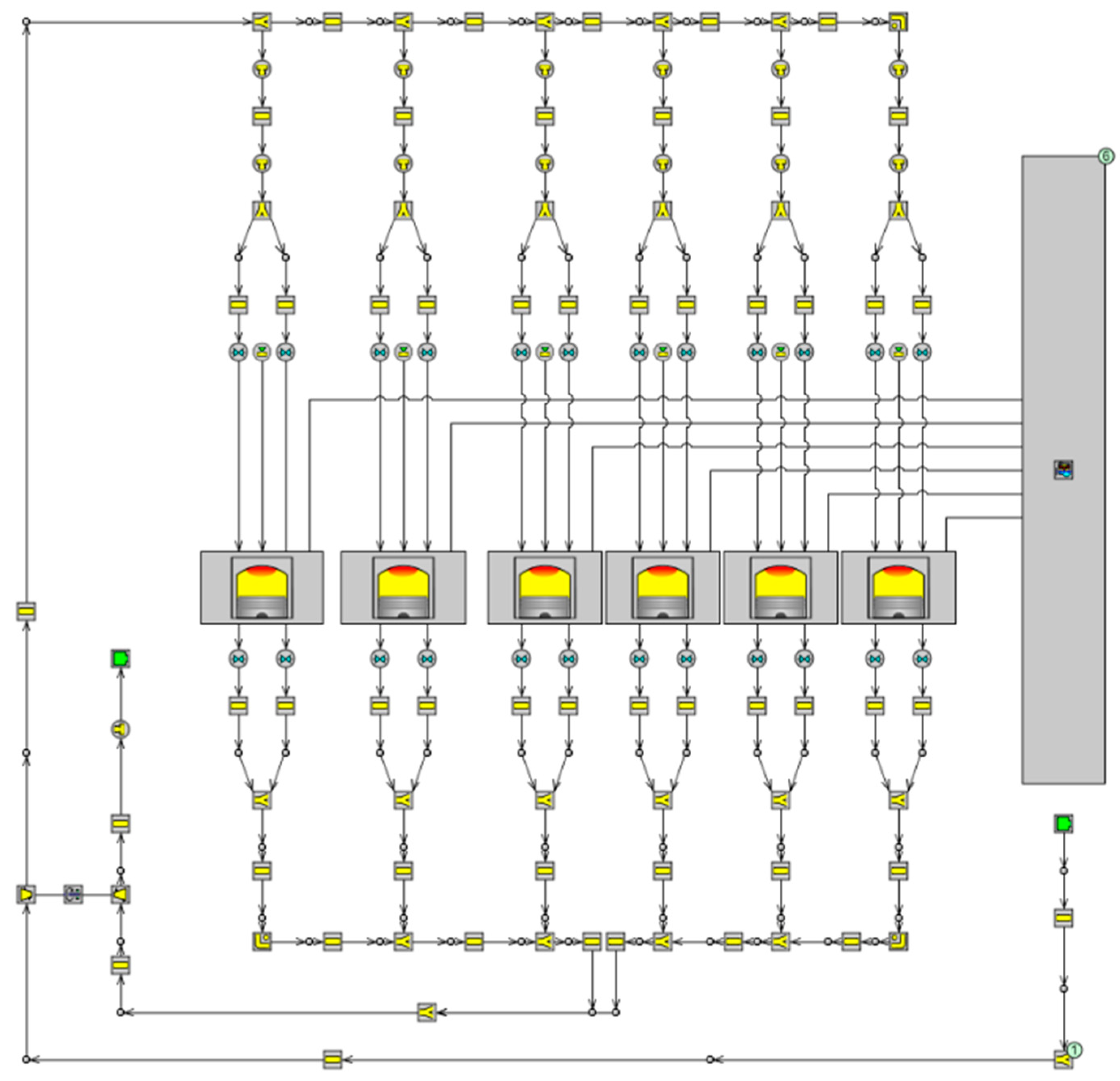
2.1. Model Establishment
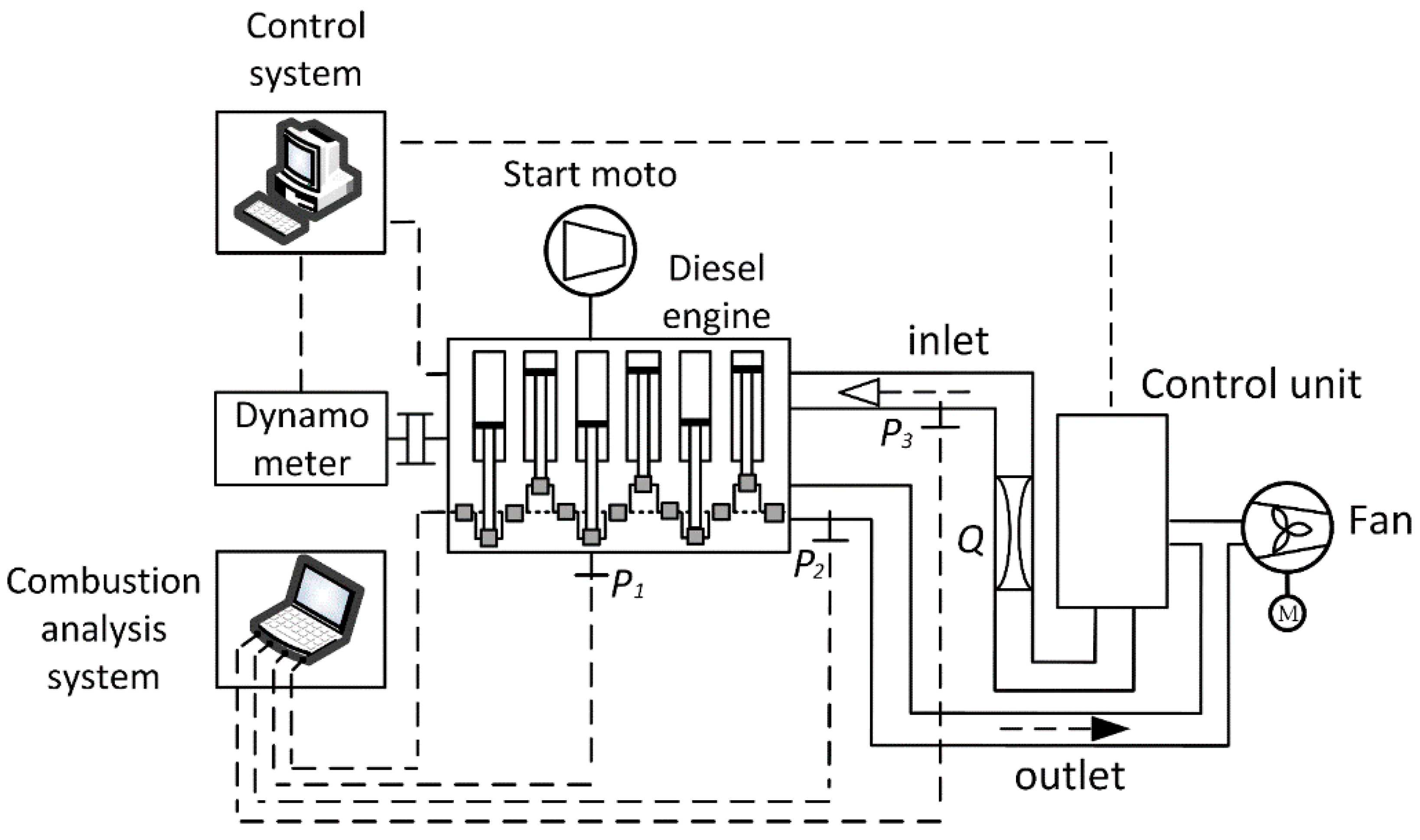
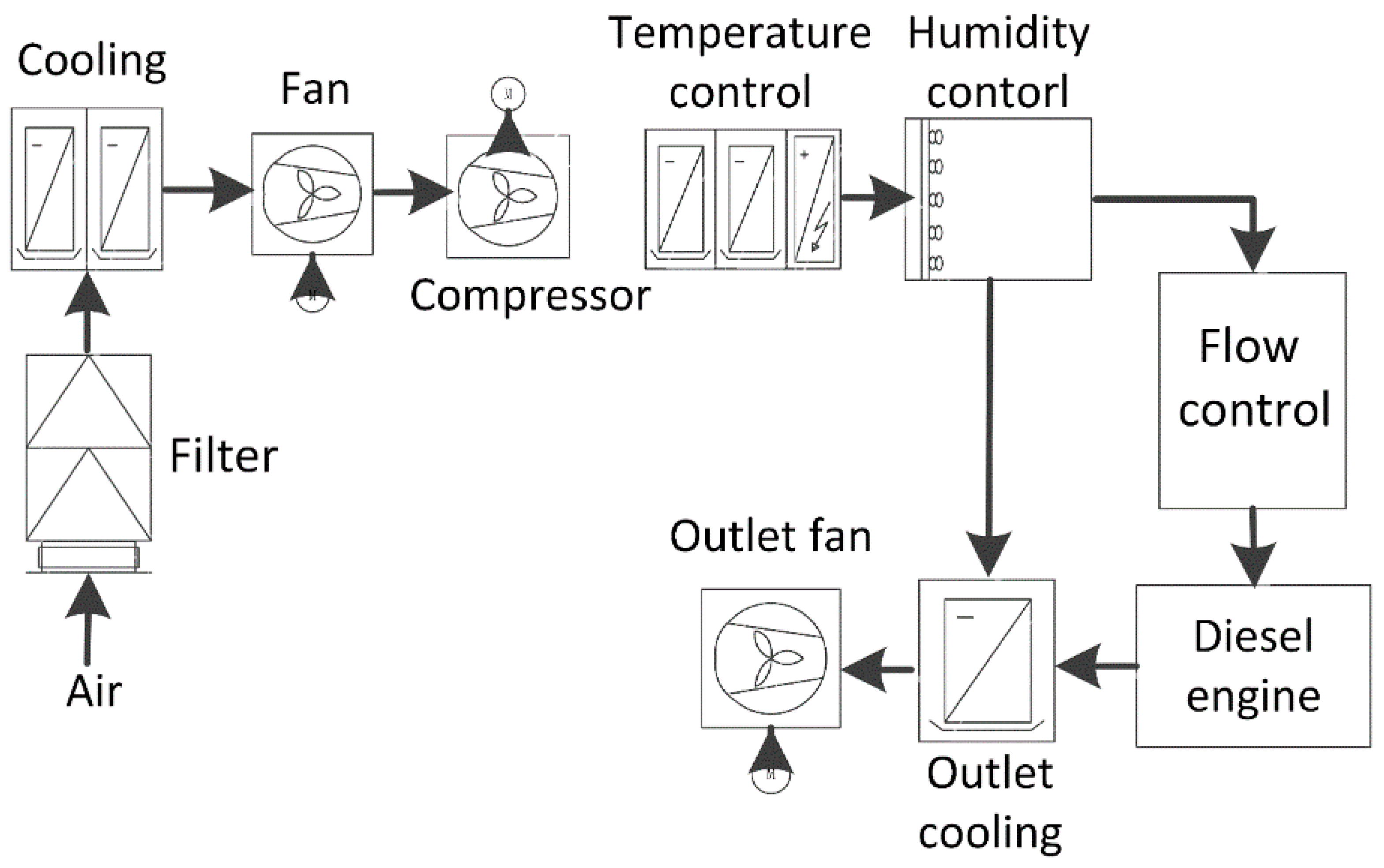
2.2. Test Equipment
2.3. Model Verification
3. Orthogonal Experiment
3.1. Orthogonal Experiment Design
3.2. Analysis of Results
4. RBFNN-Based Performance Prediction Method
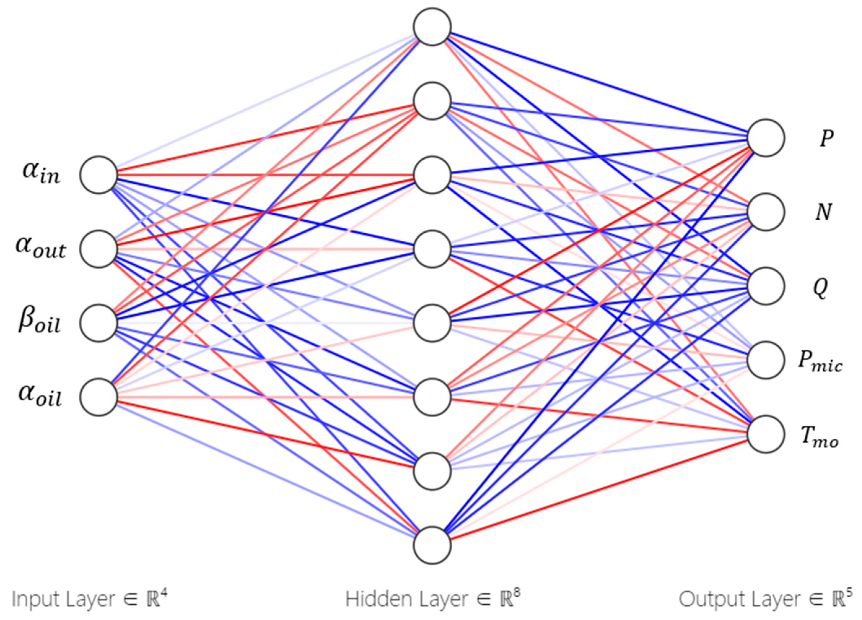
4.1. Fundamental Model
4.2. Training Samples
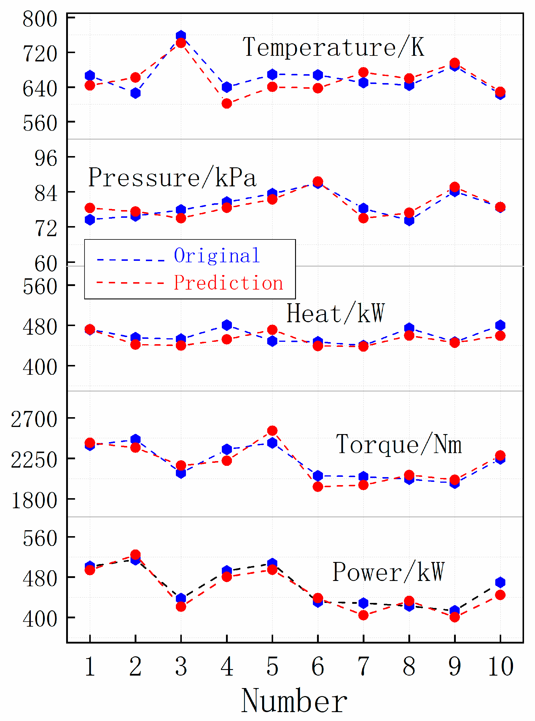
4.3. Training Results and Verification
5. RBF-NN and GACMOO Based Multi-Objective Optimization of State Parameters
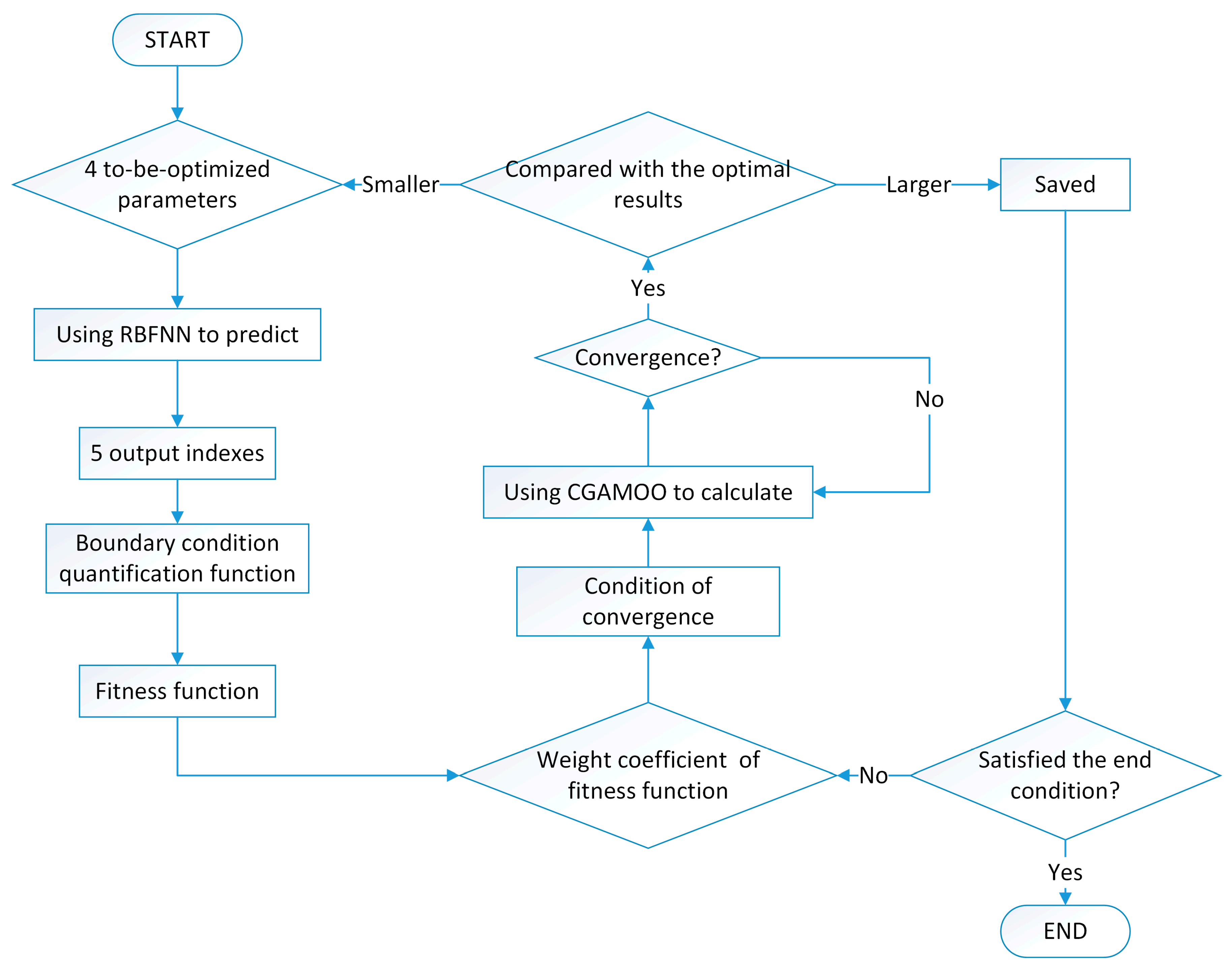
5.1. Operating Process
5.2. Boundary Condition Quantification Function
5.3. Fitness Function
5.4. Initial Value of Weight Coefficients
5.5. Updating of Weight Coefficients
- (1) Substitute weight coefficients into fitness functions of three to-be-optimized objectives for calculation;
- (2) Substitute , and in Table 10 with newest results of diesel engine’s four to-be-optimized parameters and five corresponding optimal performance indexes;
- (3) Re-arrange data in five columns of group 1, 2 and 3 in Table 10 in a descending order with as , and measuring criteria;
- (4) Set value of fitness function to be 0, and combine it with data in updated Table 10 for calculation of weight coefficients again;
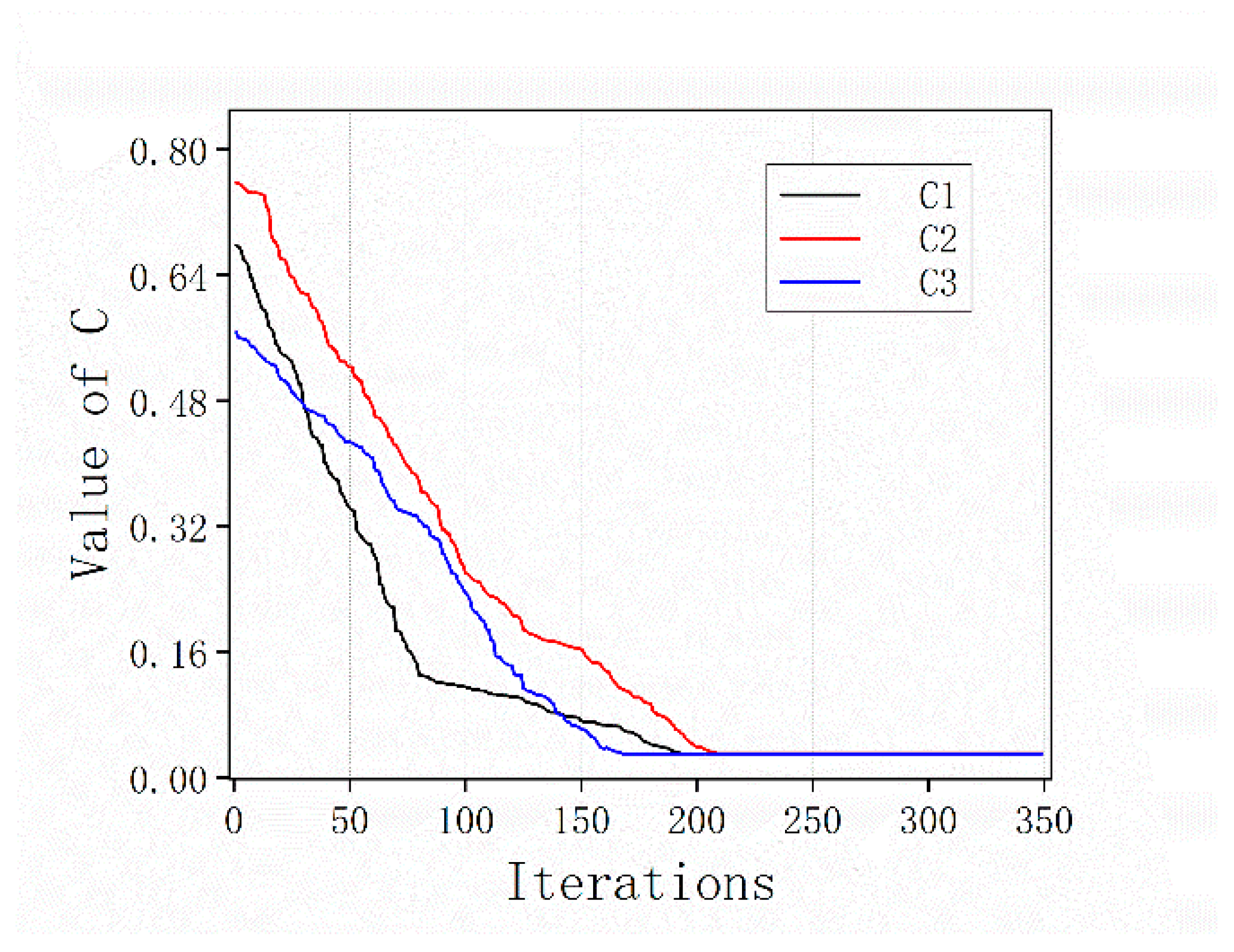
- (5) Repeat step (1) to (4) as per iterative calculation process in Figure 6 until the data satisfies the convergence condition.
5.6. Condition of Convergence
5.7. Analysis of Calculation Results
6. Verification with Bench Test
7. Conclusions
- (1)
- A simulation model is established for diesel engine working in plateau environment. Using the diesel engine bench test lab to verify the accuracy of the model.
- (2)
- Using orthogonal experiment approach to calculate and analyze the rules that how five working state parameters (inlet valve opening angle, exhaust valve opening angle, supply quantity of diesel, advance angle of injection, and compressor flow coefficient) affecting its five performance indexes (power, torque, in-cylinder heat dissipation, in-cylinder maximum pressure, and highest exhaust temperature) of diesel engine. Results indicate inlet valve opening angle, exhaust valve opening angle, supply quantity of diesel and advance angle of injection are more prominent in affecting performance indexes, thus only those four parameters are considered in subsequent calculation and analysis.
- (3)
- A prediction model is created to connect four working state parameters and five performance indexes of diesel engine on the basis of RBFNN method. The model is further trained with 221 samples which calculated from working simulation model, and predicting results are verified in term of its accuracy. Use of RBF-NN helps to serialize discrete working state parameters and corresponding performance indexes so as to facilitate the following calculation and optimization.
- (4)
- Based on the above analysis, a multi-objective optimization approach called RBFNN & GACMOO method is proposed, which is used to find the optimal working state parameters of diesel engine at 3700 m altitude and 2000 rpm condition. In this method, the boundary condition quantification function, fitness function and its weight coefficients should be identified and quantified separately.
- (5)
- Bench test verification indicates that optimal results conform to requirements of engineering accuracy. The solution can minimize in-cylinder heat dissipation and thermal load of high-temperature parts, while maintaining relatively insignificant reduction in power and torque of diesel engine working at plateau.
Author Contributions
Funding
Conflicts of Interest
Appendix A

| Number | |||||||||
|---|---|---|---|---|---|---|---|---|---|
| 1 | −0.100 | −0.100 | 184.0 | −19.80 | 539.102 | 2573.942 | 442.446 | 84.020 | 628.571 |
| 2 | −0.100 | −0.095 | 184.1 | −19.81 | 536.270 | 2560.420 | 446.218 | 83.077 | 633.820 |
| 3 | −0.100 | −0.090 | 184.2 | −19.82 | 540.706 | 2581.603 | 456.129 | 83.253 | 647.787 |
| 4 | −0.100 | −0.085 | 184.3 | −19.83 | 531.821 | 2539.181 | 454.823 | 81.376 | 645.824 |
| 5 | −0.100 | −0.080 | 184.4 | −19.84 | 526.289 | 2512.765 | 456.289 | 80.020 | 647.798 |
| 6 | −0.100 | −0.075 | 184.5 | −19.85 | 530.274 | 2531.795 | 466.064 | 80.106 | 661.568 |
| 7 | −0.100 | −0.070 | 184.6 | −19.86 | 529.003 | 2525.724 | 471.326 | 79.390 | 668.930 |
| 8 | −0.100 | −0.065 | 184.7 | −19.87 | 525.665 | 2509.786 | 474.768 | 78.361 | 673.708 |
| 9 | −0.100 | −0.060 | 184.8 | −19.88 | 512.997 | 2449.305 | 469.665 | 75.952 | 666.363 |
| 10 | −0.100 | −0.055 | 184.9 | −19.89 | 501.231 | 2393.129 | 465.161 | 73.695 | 659.872 |
| 11 | −0.100 | −0.050 | 185.0 | −19.90 | 507.822 | 2424.594 | 477.706 | 74.135 | 677.565 |
| 12 * | −0.100 | −0.045 | 185.1 | −19.91 | 501.593 | 2394.856 | 471.859 | 74.446 | 666.086 |
| 13 | −0.100 | −0.040 | 185.2 | −19.92 | 514.717 | 2457.516 | 484.217 | 77.648 | 680.258 |
| 14 | −0.100 | −0.035 | 185.3 | −19.93 | 510.485 | 2437.309 | 480.247 | 78.255 | 671.433 |
| 15 | −0.100 | −0.030 | 185.4 | −19.94 | 510.314 | 2436.493 | 480.098 | 79.474 | 667.974 |
| 16 | −0.100 | −0.025 | 185.5 | −19.95 | 511.622 | 2442.738 | 481.341 | 80.928 | 666.440 |
| 17 | −0.100 | −0.020 | 185.6 | −19.96 | 513.131 | 2449.944 | 482.772 | 82.422 | 665.147 |
| 18 | −0.100 | −0.015 | 185.7 | −19.97 | 506.703 | 2419.256 | 476.737 | 82.631 | 653.593 |
| 19 | −0.100 | −0.010 | 185.8 | −19.98 | 515.106 | 2459.375 | 484.655 | 85.264 | 661.153 |
| 20 | −0.100 | −0.005 | 185.9 | −19.99 | 512.027 | 2444.675 | 481.770 | 86.011 | 653.939 |
| 21 * | −0.100 | 0.000 | 186.0 | −20.00 | 505.106 | 2411.628 | 475.270 | 86.090 | 641.877 |
| 22 | −0.090 | 0.000 | 186.2 | −19.99 | 507.442 | 2422.781 | 480.987 | 87.423 | 651.077 |
| 23 | −0.080 | 0.000 | 186.4 | −19.98 | 498.529 | 2380.227 | 476.091 | 86.832 | 645.931 |
| 24 | −0.070 | 0.000 | 186.6 | −19.97 | 486.357 | 2322.113 | 468.027 | 85.658 | 636.464 |
| 25 | −0.060 | 0.000 | 186.8 | −19.96 | 474.142 | 2263.790 | 459.840 | 84.455 | 626.796 |
| 26 | −0.050 | 0.000 | 187.0 | −19.95 | 471.203 | 2249.761 | 460.636 | 84.901 | 629.368 |
| 27 | −0.040 | 0.000 | 187.2 | −19.94 | 458.771 | 2190.400 | 452.134 | 83.631 | 619.228 |
| 28 | −0.030 | 0.000 | 187.4 | −19.93 | 459.529 | 2194.019 | 456.645 | 84.770 | 626.917 |
| 29 | −0.020 | 0.000 | 187.6 | −19.92 | 451.304 | 2154.751 | 452.279 | 84.264 | 622.437 |
| 30 | −0.010 | 0.000 | 187.8 | −19.91 | 446.959 | 2134.007 | 451.807 | 84.485 | 623.320 |
| 31 | −0.100 | 0.050 | 187.0 | −20.10 | 515.756 | 2462.477 | 454.106 | 74.063 | 649.079 |
| 32 | −0.100 | 0.055 | 187.1 | −20.11 | 520.874 | 2486.911 | 459.173 | 75.268 | 649.948 |
| 33 | −0.100 | 0.060 | 187.2 | −20.12 | 506.445 | 2418.023 | 447.000 | 73.640 | 626.533 |
| 34 | −0.100 | 0.065 | 187.3 | −20.13 | 516.084 | 2464.043 | 456.063 | 75.506 | 632.947 |
| 35 * | −0.100 | 0.070 | 187.4 | −20.14 | 514.918 | 2458.475 | 455.586 | 75.799 | 626.026 |
| 36 | −0.100 | 0.075 | 187.5 | −20.15 | 514.574 | 2456.832 | 455.835 | 76.211 | 620.124 |
| 37 | −0.100 | 0.080 | 187.6 | −20.16 | 522.099 | 2492.761 | 463.062 | 77.794 | 623.635 |
| 38 | −0.100 | 0.085 | 187.7 | −20.17 | 521.798 | 2491.327 | 463.355 | 78.218 | 617.727 |
| 39 | −0.100 | 0.090 | 187.8 | −20.18 | 513.222 | 2450.378 | 456.289 | 77.393 | 602.121 |
| 40 | −0.100 | 0.095 | 187.9 | −20.19 | 508.442 | 2427.556 | 452.584 | 77.127 | 591.116 |
| 41 | −0.100 | 0.100 | 188.0 | −20.20 | 518.199 | 2474.143 | 461.823 | 79.071 | 596.965 |
| 42 | −0.095 | 0.080 | 187.7 | −20.18 | 504.367 | 2408.099 | 459.241 | 78.402 | 591.619 |
| 43 | −0.090 | 0.060 | 187.4 | −20.16 | 491.539 | 2346.854 | 457.441 | 77.869 | 587.307 |
| 44 | −0.085 | 0.040 | 187.1 | −20.14 | 489.885 | 2338.958 | 466.153 | 79.123 | 596.470 |
| 45 | −0.080 | 0.020 | 186.8 | −20.12 | 478.885 | 2286.438 | 466.126 | 78.891 | 594.421 |
| 46 | −0.075 | 0.000 | 186.5 | −20.10 | 475.640 | 2270.944 | 473.781 | 79.956 | 602.144 |
| 47 | −0.070 | −0.020 | 186.2 | −20.08 | 457.149 | 2182.657 | 466.210 | 78.452 | 590.522 |
| 48 * | −0.065 | −0.040 | 185.9 | −20.06 | 455.007 | 2172.431 | 475.307 | 79.753 | 600.012 |
| 49 | −0.060 | −0.060 | 185.6 | −20.04 | 433.346 | 2069.010 | 463.914 | 77.618 | 583.656 |
| 50 | −0.055 | −0.080 | 185.3 | −20.02 | 421.109 | 2010.583 | 462.242 | 77.116 | 579.593 |
| 51 | −0.050 | −0.100 | 185.0 | −20.00 | 417.989 | 1995.689 | 470.706 | 78.304 | 588.217 |
| 52 | −0.050 | −0.095 | 185.1 | −20.01 | 420.116 | 2005.842 | 468.714 | 78.247 | 606.857 |
| 53 | −0.050 | −0.090 | 185.2 | −20.02 | 417.701 | 1994.311 | 461.693 | 77.348 | 618.801 |
| 54 | −0.050 | −0.085 | 185.3 | −20.03 | 415.550 | 1984.041 | 455.046 | 76.507 | 630.843 |
| 55 | −0.050 | −0.080 | 185.4 | −20.04 | 432.640 | 2065.642 | 469.351 | 79.196 | 672.517 |
| 56 | −0.050 | −0.075 | 185.5 | −20.05 | 419.552 | 2003.151 | 450.910 | 76.360 | 667.301 |
| 57 | −0.050 | −0.070 | 185.6 | −20.06 | 435.926 | 2081.327 | 464.136 | 78.886 | 708.939 |
| 58 | −0.050 | −0.065 | 185.7 | −20.07 | 429.338 | 2049.873 | 452.849 | 77.251 | 713.462 |
| 59 | −0.050 | −0.060 | 185.8 | −20.08 | 427.195 | 2039.644 | 446.372 | 76.428 | 724.944 |
| 60 * | −0.050 | −0.055 | 185.9 | −20.09 | 437.493 | 2088.808 | 452.847 | 77.826 | 757.700 |
| 61 | −0.050 | −0.050 | 186.0 | −20.10 | 435.060 | 2077.195 | 446.102 | 76.954 | 768.566 |
| 62 | −0.050 | −0.045 | 186.1 | −20.11 | 428.268 | 2044.764 | 441.714 | 75.825 | 743.148 |
| 63 | −0.050 | −0.040 | 186.2 | −20.12 | 425.214 | 2030.183 | 441.150 | 75.357 | 724.381 |
| 64 | −0.050 | −0.035 | 186.3 | −20.13 | 432.407 | 2064.525 | 451.271 | 76.707 | 722.789 |
| 65 | −0.050 | −0.030 | 186.4 | −20.14 | 425.435 | 2031.241 | 446.640 | 75.544 | 697.364 |
| 66 | −0.050 | −0.025 | 186.5 | −20.15 | 423.072 | 2019.958 | 446.818 | 75.200 | 679.643 |
| 67 | −0.050 | −0.020 | 186.6 | −20.16 | 428.779 | 2047.204 | 455.570 | 76.291 | 674.620 |
| 68 | −0.050 | −0.015 | 186.7 | −20.17 | 421.022 | 2010.170 | 450.034 | 74.987 | 648.327 |
| 69 | −0.050 | −0.010 | 186.8 | −20.18 | 418.245 | 1996.911 | 449.784 | 74.568 | 629.896 |
| 70 | −0.050 | −0.005 | 186.9 | −20.19 | 406.757 | 1942.063 | 440.103 | 72.595 | 598.673 |
| 71 | −0.050 | 0.000 | 187.0 | −20.2 | 411.628 | 1965.316 | 448.109 | 73.542 | 591.593 |
| 72 * | −0.050 | 0.005 | 187.1 | −20.16 | 414.409 | 1978.597 | 444.221 | 72.455 | 585.506 |
| 73 | −0.050 | 0.010 | 187.2 | −20.12 | 436.443 | 2083.798 | 460.853 | 74.708 | 606.449 |
| 74 | −0.050 | 0.015 | 187.3 | −20.08 | 432.215 | 2063.611 | 449.745 | 72.464 | 590.887 |
| 75 | −0.050 | 0.020 | 187.4 | −20.04 | 442.358 | 2112.039 | 453.767 | 72.669 | 595.228 |
| 76 | −0.050 | 0.025 | 187.5 | −20.00 | 452.735 | 2161.585 | 457.982 | 72.902 | 599.816 |
| 77 | −0.050 | 0.030 | 187.6 | −19.96 | 459.834 | 2195.479 | 458.880 | 72.607 | 600.058 |
| 78 | −0.050 | 0.035 | 187.7 | −19.92 | 468.496 | 2236.834 | 461.358 | 72.564 | 602.371 |
| 79 | −0.050 | 0.040 | 187.8 | −19.88 | 478.888 | 2286.451 | 465.518 | 72.783 | 606.877 |
| 80 | −0.050 | 0.045 | 187.9 | −19.84 | 485.888 | 2319.871 | 466.380 | 72.487 | 607.082 |
| 81 | −0.050 | 0.050 | 188.0 | −19.8 | 499.071 | 2382.812 | 473.144 | 73.105 | 614.965 |
| 82 | −0.050 | 0.055 | 187.6 | −19.81 | 494.763 | 2362.248 | 473.569 | 75.219 | 620.507 |
| 83 | −0.050 | 0.060 | 187.2 | −19.82 | 494.081 | 2358.990 | 477.518 | 77.918 | 630.726 |
| 84 * | −0.050 | 0.065 | 186.8 | −19.83 | 492.336 | 2350.660 | 480.521 | 80.498 | 639.783 |
| 85 | −0.050 | 0.070 | 186.4 | −19.84 | 475.930 | 2272.328 | 469.145 | 80.638 | 629.620 |
| 86 | −0.050 | 0.075 | 186.0 | −19.85 | 465.163 | 2220.918 | 463.166 | 81.636 | 626.530 |
| 87 | −0.050 | 0.080 | 185.6 | −19.86 | 473.326 | 2259.893 | 476.121 | 86.008 | 649.140 |
| 88 | −0.050 | 0.085 | 185.2 | −19.87 | 464.431 | 2217.427 | 472.021 | 87.343 | 648.607 |
| 89 | −0.050 | 0.090 | 184.8 | −19.88 | 453.291 | 2164.238 | 465.543 | 88.198 | 644.705 |
| 90 | −0.050 | 0.095 | 184.4 | −19.89 | 448.079 | 2139.356 | 465.094 | 90.169 | 649.094 |
| 91 | −0.050 | 0.100 | 184.0 | −19.90 | 444.772 | 2123.565 | 466.648 | 92.540 | 656.302 |
| 92 | −0.045 | 0.080 | 184.2 | −19.93 | 445.038 | 2124.835 | 467.741 | 91.481 | 658.338 |
| 93 | −0.040 | 0.060 | 184.4 | −19.96 | 450.533 | 2151.072 | 474.345 | 91.476 | 668.139 |
| 94 | −0.035 | 0.040 | 184.6 | −19.99 | 438.784 | 2094.975 | 462.786 | 87.980 | 652.351 |
| 95 | −0.030 | 0.020 | 184.8 | −20.02 | 446.968 | 2134.050 | 472.249 | 88.484 | 666.195 |
| 96 | −0.025 | 0.000 | 185.0 | −20.05 | 435.131 | 2077.532 | 460.555 | 85.028 | 650.192 |
| 97 | −0.020 | −0.020 | 185.2 | −20.08 | 443.189 | 2116.005 | 469.916 | 85.464 | 663.912 |
| 98 * | −0.015 | −0.040 | 185.4 | −20.11 | 428.283 | 2044.835 | 454.919 | 81.482 | 643.213 |
| 99 | −0.010 | −0.060 | 185.6 | −20.14 | 443.389 | 2116.960 | 471.807 | 83.205 | 667.598 |
| 100 | −0.005 | −0.080 | 185.8 | −20.17 | 435.256 | 2078.129 | 463.983 | 80.542 | 657.028 |
| 101 | 0.000 | −0.100 | 186.0 | −20.20 | 433.272 | 2068.658 | 462.699 | 79.037 | 655.711 |
| 102 | 0.000 | −0.095 | 186.1 | −20.16 | 438.555 | 2093.882 | 458.243 | 79.003 | 652.932 |
| 103 | 0.000 | −0.090 | 186.2 | −20.12 | 446.871 | 2133.586 | 456.984 | 79.518 | 654.697 |
| 104 | 0.000 | −0.085 | 186.3 | −20.08 | 448.202 | 2139.939 | 448.691 | 78.800 | 646.346 |
| 105 | 0.000 | −0.080 | 186.4 | −20.04 | 462.791 | 2209.595 | 453.648 | 80.412 | 657.090 |
| 106 | 0.000 | −0.075 | 186.5 | −20.00 | 465.942 | 2224.642 | 447.330 | 80.030 | 651.527 |
| 107 | 0.000 | −0.070 | 186.6 | −19.96 | 473.533 | 2260.882 | 445.353 | 80.418 | 652.256 |
| 108 | 0.000 | −0.065 | 186.7 | −19.92 | 477.424 | 2279.462 | 439.958 | 80.184 | 647.954 |
| 109 | 0.000 | −0.060 | 186.8 | −19.88 | 485.096 | 2316.091 | 438.105 | 80.591 | 648.845 |
| 110 * | 0.000 | −0.055 | 186.9 | −19.84 | 507.266 | 2421.943 | 449.073 | 83.379 | 668.839 |
| 111 | 0.000 | −0.050 | 187.0 | −19.8 | 507.444 | 2422.792 | 440.439 | 82.539 | 659.692 |
| 112 | 0.000 | −0.045 | 187.1 | −19.81 | 502.758 | 2400.418 | 443.057 | 83.043 | 658.460 |
| 113 | 0.000 | −0.040 | 187.2 | −19.82 | 501.649 | 2395.121 | 448.936 | 84.157 | 661.993 |
| 114 | 0.000 | −0.035 | 187.3 | −19.83 | 477.620 | 2280.398 | 434.147 | 81.397 | 635.166 |
| 115 | 0.000 | −0.030 | 187.4 | −19.84 | 485.300 | 2317.065 | 448.147 | 84.035 | 650.483 |
| 116 | 0.000 | −0.025 | 187.5 | −19.85 | 477.677 | 2280.670 | 448.218 | 84.061 | 645.435 |
| 117 | 0.000 | −0.020 | 187.6 | −19.86 | 471.945 | 2253.301 | 450.073 | 84.422 | 642.949 |
| 118 | 0.000 | −0.015 | 187.7 | −19.87 | 450.064 | 2148.829 | 436.312 | 81.853 | 618.306 |
| 119 | 0.000 | −0.010 | 187.8 | −19.88 | 446.239 | 2130.566 | 439.865 | 82.531 | 618.330 |
| 120 | 0.000 | −0.005 | 187.9 | −19.89 | 444.939 | 2124.359 | 446.048 | 83.704 | 621.956 |
| 121 | 0.000 | 0.000 | 188.0 | −19.90 | 438.336 | 2092.835 | 447.014 | 83.898 | 618.242 |
| 122 * | 0.000 | 0.005 | 187.6 | −19.91 | 441.460 | 2107.748 | 450.789 | 85.038 | 626.993 |
| 123 | 0.000 | 0.010 | 187.2 | −19.92 | 429.012 | 2048.320 | 438.652 | 83.168 | 613.551 |
| 124 | 0.000 | 0.015 | 186.8 | −19.93 | 437.432 | 2088.519 | 447.848 | 85.340 | 629.924 |
| 125 | 0.000 | 0.020 | 186.4 | −19.94 | 442.048 | 2110.558 | 453.169 | 86.788 | 640.962 |
| 126 | 0.000 | 0.025 | 186.0 | −19.95 | 436.067 | 2082.000 | 447.625 | 86.155 | 636.633 |
| 127 | 0.000 | 0.030 | 185.6 | −19.96 | 437.838 | 2090.458 | 450.036 | 87.050 | 643.593 |
| 128 | 0.000 | 0.035 | 185.2 | −19.97 | 433.071 | 2067.699 | 445.725 | 86.644 | 640.926 |
| 129 | 0.000 | 0.040 | 184.8 | −19.98 | 437.087 | 2086.874 | 450.453 | 87.995 | 651.263 |
| 130 | 0.000 | 0.045 | 184.4 | −19.99 | 439.796 | 2099.807 | 453.845 | 89.093 | 659.732 |
| 131 | 0.000 | 0.050 | 184.0 | −20.00 | 431.890 | 2062.058 | 446.278 | 88.036 | 652.239 |
| 132 | 0.000 | 0.055 | 184.1 | −20.01 | 432.261 | 2063.832 | 447.258 | 87.894 | 657.045 |
| 133 | 0.000 | 0.060 | 184.2 | −20.02 | 432.100 | 2063.064 | 447.686 | 87.644 | 661.040 |
| 134 | 0.000 | 0.065 | 184.3 | −20.03 | 437.175 | 2087.291 | 453.545 | 88.454 | 673.088 |
| 135 * | 0.000 | 0.070 | 184.4 | −20.04 | 430.908 | 2057.369 | 447.636 | 86.970 | 667.659 |
| 136 | 0.000 | 0.075 | 184.5 | −20.05 | 441.041 | 2105.752 | 458.769 | 88.795 | 687.675 |
| 137 | 0.000 | 0.080 | 184.6 | −20.06 | 440.570 | 2103.503 | 458.883 | 88.480 | 691.247 |
| 138 | 0.000 | 0.085 | 184.7 | −20.07 | 428.063 | 2043.787 | 446.443 | 85.754 | 675.803 |
| 139 | 0.000 | 0.090 | 184.8 | −20.08 | 429.063 | 2048.560 | 448.073 | 85.740 | 681.567 |
| 140 | 0.000 | 0.095 | 184.9 | −20.09 | 441.691 | 2108.853 | 461.865 | 88.044 | 705.931 |
| 141 | 0.000 | 0.100 | 185.0 | −20.10 | 433.986 | 2072.067 | 454.402 | 86.292 | 697.843 |
| 142 | 0.005 | 0.080 | 185.2 | −20.08 | 433.094 | 2067.809 | 453.495 | 84.840 | 689.066 |
| 143 | 0.010 | 0.060 | 185.4 | −20.06 | 429.127 | 2048.867 | 449.368 | 82.801 | 675.478 |
| 144 | 0.015 | 0.040 | 185.6 | −20.04 | 438.779 | 2094.952 | 459.504 | 83.372 | 683.230 |
| 145 | 0.020 | 0.020 | 185.8 | −20.02 | 429.856 | 2052.345 | 450.186 | 80.412 | 662.044 |
| 146 * | 0.025 | 0.000 | 186.0 | −20.00 | 432.012 | 2062.639 | 452.471 | 79.543 | 658.036 |
| 147 | 0.030 | −0.020 | 186.2 | −19.98 | 432.260 | 2063.823 | 452.759 | 78.317 | 651.080 |
| 148 | 0.035 | −0.040 | 186.4 | −19.96 | 427.376 | 2040.505 | 447.671 | 76.173 | 636.471 |
| 149 | 0.040 | −0.060 | 186.6 | −19.94 | 433.600 | 2070.224 | 454.218 | 76.006 | 638.382 |
| 150 | 0.045 | −0.080 | 186.8 | −19.92 | 427.689 | 2042.001 | 448.053 | 73.710 | 622.419 |
| 151 | 0.050 | −0.100 | 187.0 | −19.90 | 433.639 | 2070.409 | 454.314 | 73.458 | 623.716 |
| 152 | 0.050 | −0.095 | 187.1 | −19.91 | 434.673 | 2075.345 | 454.106 | 74.465 | 630.109 |
| 153 | 0.050 | −0.090 | 187.2 | −19.92 | 439.307 | 2097.469 | 457.644 | 76.097 | 641.778 |
| 154 | 0.050 | −0.085 | 187.3 | −19.93 | 441.766 | 2109.212 | 458.897 | 77.366 | 650.343 |
| 155 | 0.050 | −0.080 | 187.4 | −19.94 | 428.543 | 2046.077 | 443.893 | 75.866 | 635.694 |
| 156 | 0.050 | −0.075 | 187.5 | −19.95 | 427.125 | 2039.308 | 441.163 | 76.427 | 638.386 |
| 157 | 0.050 | −0.070 | 187.6 | −19.96 | 429.764 | 2051.909 | 442.621 | 77.716 | 647.148 |
| 158 * | 0.050 | −0.065 | 187.7 | −19.97 | 428.579 | 2046.251 | 440.137 | 78.314 | 650.162 |
| 159 | 0.050 | −0.060 | 187.8 | −19.98 | 434.792 | 2075.916 | 445.239 | 80.273 | 664.449 |
| 160 | 0.050 | −0.055 | 187.9 | −19.99 | 439.951 | 2100.546 | 449.228 | 82.058 | 677.245 |
| 161 | 0.050 | −0.050 | 188.0 | −20.00 | 436.549 | 2084.302 | 444.473 | 82.248 | 676.876 |
| 162 | 0.050 | −0.045 | 187.6 | −20.01 | 436.311 | 2083.169 | 445.624 | 83.355 | 674.778 |
| 163 | 0.050 | −0.040 | 187.2 | −20.02 | 446.239 | 2130.567 | 457.184 | 86.425 | 688.369 |
| 164 | 0.050 | −0.035 | 186.8 | −20.03 | 441.326 | 2107.113 | 453.550 | 86.631 | 679.053 |
| 165 | 0.050 | −0.030 | 186.4 | −20.04 | 440.192 | 2101.696 | 453.776 | 87.558 | 675.580 |
| 166 | 0.050 | −0.025 | 186.0 | −20.05 | 437.098 | 2086.924 | 451.963 | 88.081 | 669.122 |
| 167 | 0.050 | −0.020 | 185.6 | −20.06 | 448.304 | 2140.429 | 464.958 | 91.503 | 684.530 |
| 168 | 0.050 | −0.015 | 185.2 | −20.07 | 434.778 | 2075.848 | 452.290 | 89.867 | 662.187 |
| 169 | 0.050 | −0.010 | 184.8 | −20.08 | 450.738 | 2152.051 | 470.299 | 94.329 | 684.750 |
| 170 * | 0.050 | −0.005 | 184.4 | −20.09 | 440.920 | 2105.172 | 461.425 | 93.407 | 668.132 |
| 171 | 0.050 | 0.000 | 184.0 | −20.10 | 443.854 | 2119.180 | 465.871 | 95.166 | 670.871 |
| 172 | 0.050 | 0.005 | 184.1 | −20.11 | 441.862 | 2109.672 | 468.230 | 93.229 | 670.283 |
| 173 | 0.050 | 0.010 | 184.2 | −20.12 | 439.624 | 2098.986 | 470.354 | 91.232 | 669.335 |
| 174 | 0.050 | 0.015 | 184.3 | −20.13 | 434.976 | 2076.791 | 469.899 | 88.734 | 664.716 |
| 175 | 0.050 | 0.020 | 184.4 | −20.14 | 435.351 | 2078.585 | 474.899 | 87.252 | 667.792 |
| 176 | 0.050 | 0.025 | 184.5 | −20.15 | 425.565 | 2031.862 | 468.787 | 83.743 | 655.264 |
| 177 | 0.050 | 0.030 | 184.6 | −20.16 | 419.156 | 2001.263 | 466.294 | 80.932 | 647.882 |
| 178 | 0.050 | 0.035 | 184.7 | −20.17 | 421.140 | 2010.734 | 473.164 | 79.733 | 653.487 |
| 179 | 0.050 | 0.040 | 184.8 | −20.18 | 422.307 | 2016.303 | 479.227 | 78.342 | 657.884 |
| 180 | 0.050 | 0.045 | 184.9 | −20.19 | 417.043 | 1991.172 | 478.025 | 75.747 | 652.281 |
| 181 | 0.050 | 0.050 | 185.0 | −20.20 | 409.677 | 1956.001 | 474.346 | 72.792 | 643.354 |
| 182 * | 0.050 | 0.055 | 185.1 | −20.16 | 422.704 | 2018.201 | 474.331 | 74.228 | 644.324 |
| 183 | 0.050 | 0.060 | 185.2 | −20.12 | 426.643 | 2037.008 | 464.304 | 74.079 | 631.683 |
| 184 | 0.050 | 0.065 | 185.3 | −20.08 | 445.843 | 2128.680 | 470.868 | 76.578 | 641.615 |
| 185 | 0.050 | 0.070 | 185.4 | −20.04 | 448.249 | 2140.165 | 459.714 | 76.194 | 627.402 |
| 186 | 0.050 | 0.075 | 185.5 | −20.00 | 472.337 | 2255.173 | 470.685 | 79.489 | 643.393 |
| 187 | 0.050 | 0.080 | 185.6 | −19.96 | 484.904 | 2315.175 | 469.774 | 80.822 | 643.173 |
| 188 | 0.050 | 0.085 | 185.7 | −19.92 | 481.593 | 2299.364 | 453.838 | 79.529 | 622.354 |
| 189 | 0.050 | 0.090 | 185.8 | −19.88 | 502.060 | 2397.086 | 460.455 | 82.171 | 632.450 |
| 190 | 0.050 | 0.095 | 185.9 | −19.84 | 509.058 | 2430.499 | 454.592 | 82.601 | 625.415 |
| 191 | 0.050 | 0.100 | 186.0 | −19.80 | 522.206 | 2493.273 | 454.277 | 84.033 | 626.009 |
| 192 | 0.055 | 0.080 | 186.2 | −19.83 | 515.216 | 2459.900 | 456.973 | 84.186 | 633.892 |
| 193 | 0.060 | 0.060 | 186.4 | −19.86 | 495.097 | 2363.842 | 447.887 | 82.174 | 625.371 |
| 194 * | 0.065 | 0.040 | 186.6 | −19.89 | 497.580 | 2375.697 | 459.283 | 83.918 | 645.462 |
| 195 | 0.070 | 0.020 | 186.8 | −19.92 | 489.354 | 2336.423 | 461.051 | 83.893 | 652.136 |
| 196 | 0.075 | 0.000 | 187.0 | −19.95 | 469.128 | 2239.852 | 451.336 | 81.786 | 642.492 |
| 197 | 0.080 | −0.020 | 187.2 | −19.98 | 457.320 | 2183.476 | 449.463 | 81.109 | 643.901 |
| 198 | 0.085 | −0.040 | 187.4 | −20.01 | 455.046 | 2172.618 | 457.072 | 82.139 | 658.939 |
| 199 | 0.090 | −0.060 | 187.6 | −20.04 | 435.982 | 2081.596 | 447.766 | 80.130 | 649.573 |
| 200 | 0.095 | −0.080 | 187.8 | −20.07 | 429.609 | 2051.167 | 451.353 | 80.434 | 658.853 |
| 201 | 0.100 | −0.100 | 188.0 | −20.10 | 425.114 | 2029.706 | 457.115 | 81.119 | 671.388 |
| 202 | 0.100 | −0.095 | 187.6 | −20.11 | 425.553 | 2031.803 | 458.094 | 82.278 | 679.348 |
| 203 | 0.100 | −0.090 | 187.2 | −20.12 | 428.094 | 2043.934 | 461.343 | 83.859 | 690.766 |
| 204 | 0.100 | −0.085 | 186.8 | −20.13 | 419.525 | 2003.024 | 452.616 | 83.256 | 684.205 |
| 205 | 0.100 | −0.080 | 186.4 | −20.14 | 424.794 | 2028.180 | 458.817 | 85.398 | 700.208 |
| 206 * | 0.100 | −0.075 | 186.0 | −20.15 | 413.241 | 1973.021 | 446.846 | 84.150 | 688.425 |
| 207 | 0.100 | −0.070 | 185.6 | −20.16 | 417.281 | 1992.308 | 451.729 | 86.065 | 702.539 |
| 208 | 0.100 | −0.065 | 185.2 | −20.17 | 418.252 | 1996.946 | 453.301 | 87.369 | 711.629 |
| 209 | 0.100 | −0.060 | 184.8 | −20.18 | 409.455 | 1954.945 | 444.280 | 86.619 | 704.013 |
| 210 | 0.100 | −0.055 | 184.4 | −20.19 | 411.802 | 1966.147 | 447.345 | 88.217 | 715.494 |
| 211 | 0.100 | −0.050 | 184.0 | −20.20 | 410.100 | 1958.022 | 446.018 | 88.958 | 720.008 |
| 212 | 0.100 | −0.045 | 184.1 | −20.16 | 417.385 | 1992.804 | 445.067 | 87.532 | 703.968 |
| 213 | 0.100 | −0.040 | 184.2 | −20.12 | 426.837 | 2037.933 | 446.519 | 86.591 | 691.882 |
| 214 | 0.100 | −0.035 | 184.3 | −20.08 | 435.874 | 2081.079 | 447.588 | 85.583 | 679.288 |
| 215 | 0.100 | −0.030 | 184.4 | −20.04 | 451.615 | 2156.238 | 455.473 | 85.869 | 676.921 |
| 216 | 0.100 | −0.025 | 184.5 | −20.00 | 457.493 | 2184.302 | 453.400 | 84.275 | 659.735 |
| 217 * | 0.100 | −0.020 | 184.6 | −19.96 | 481.972 | 2301.173 | 469.608 | 86.057 | 668.876 |
| 218 | 0.100 | −0.015 | 184.7 | −19.92 | 483.110 | 2306.608 | 463.001 | 83.646 | 645.388 |
| 219 | 0.100 | −0.010 | 184.8 | −19.88 | 488.974 | 2334.607 | 461.148 | 82.129 | 628.941 |
| 220 | 0.100 | −0.005 | 184.9 | −19.84 | 509.723 | 2433.673 | 473.253 | 83.085 | 631.383 |
| 221 | 0.100 | 0.000 | 185.0 | −19.80 | 516.548 | 2466.257 | 472.338 | 81.741 | 616.278 |
| 222 | 0.100 | 0.005 | 185.1 | −19.81 | 511.380 | 2441.583 | 473.848 | 81.457 | 617.829 |
| 223 | 0.100 | 0.010 | 185.2 | −19.82 | 494.387 | 2360.451 | 464.296 | 79.280 | 604.965 |
| 224 | 0.100 | 0.015 | 185.3 | −19.83 | 504.046 | 2406.566 | 479.858 | 81.384 | 624.818 |
| 225 | 0.100 | 0.020 | 185.4 | −19.84 | 495.208 | 2364.370 | 478.002 | 80.518 | 621.979 |
| 226 | 0.100 | 0.025 | 185.5 | −19.85 | 476.074 | 2273.013 | 466.018 | 77.962 | 605.973 |
| 227 | 0.100 | 0.030 | 185.6 | −19.86 | 481.002 | 2296.544 | 477.585 | 79.346 | 620.591 |
| 228 | 0.100 | 0.035 | 185.7 | −19.87 | 460.046 | 2196.490 | 463.417 | 76.457 | 601.772 |
| 229 * | 0.100 | 0.040 | 185.8 | −19.88 | 469.805 | 2243.085 | 480.232 | 78.676 | 623.181 |
| 230 | 0.100 | 0.045 | 185.9 | −19.89 | 455.612 | 2175.321 | 472.703 | 76.897 | 612.992 |
| 231 | 0.100 | 0.050 | 186.0 | −19.90 | 447.409 | 2136.156 | 471.257 | 76.117 | 610.700 |
| 232 | 0.100 | 0.055 | 186.1 | −19.91 | 451.170 | 2154.112 | 476.258 | 77.807 | 623.612 |
| 233 | 0.100 | 0.060 | 186.2 | −19.92 | 437.730 | 2089.940 | 463.092 | 76.523 | 612.683 |
| 234 | 0.100 | 0.065 | 186.3 | −19.93 | 435.036 | 2077.077 | 461.272 | 77.093 | 616.617 |
| 235 | 0.100 | 0.070 | 186.4 | −19.94 | 436.906 | 2086.006 | 464.303 | 78.484 | 627.111 |
| 236 | 0.100 | 0.075 | 186.5 | −19.95 | 438.642 | 2094.295 | 467.215 | 79.874 | 637.585 |
| 237 | 0.100 | 0.080 | 186.6 | −19.96 | 421.193 | 2010.988 | 449.669 | 77.747 | 619.994 |
| 238 * | 0.100 | 0.085 | 186.7 | −19.97 | 418.885 | 1999.968 | 448.252 | 78.380 | 624.433 |
| 239 | 0.100 | 0.090 | 186.8 | −19.98 | 432.048 | 2062.814 | 463.433 | 81.950 | 652.251 |
| 240 | 0.100 | 0.095 | 186.9 | −19.99 | 428.435 | 2045.561 | 460.659 | 82.378 | 655.037 |
| 241 | 0.100 | 0.100 | 187.0 | −20.00 | 417.703 | 1994.322 | 450.209 | 81.416 | 646.779 |
References
- Zhu, Z.; Zhang, F.; Li, C.; Wu, T.; Han, K.; Lv, J.; Li, Y.; Xiao, X. Genetic algorithm optimization applied to the fuel supply parameters of diesel engines working at plateau. Appl. Energy 2015, 157, 789–797. [Google Scholar] [CrossRef]
- Huaiqing, Z. Research on Power Enhancement of 16V280ZJA Diesel Engine for Plateau Locomotive. Master’s Thesis, Shanghai Jiaotong University, Shanghai, China, 2007. [Google Scholar]
- Qiangqiang, T.; Deyuan, W.; Chengguan, W.; Yuan, L.; Diming, L.; Yunguang, L.; Sheng, L.; Zhenhuan, Y. Research on Performance Optimization of Heavy-duty Diesel Engines in Plateau Environment. Ordnance Ind. 2018, 39, 436–443. [Google Scholar]
- Zhang, H.; Zhang, H.; Wang, Z. Effect on Vehicle Turbocharger Exhaust Gas Energy Utilization for the Performance of Centrifugal Compressors under Plateau Conditions. Energies 2017, 10, 2121. [Google Scholar] [CrossRef] [Green Version]
- Xia, M.; Zhao, C.; Zhang, F.; Huang, Y. Modeling the Performance of a New Speed Adjustable Compound Supercharging Diesel Engine Working under Plateau Conditions. Energies 2017, 10, 689. [Google Scholar]
- Qiao, Y.; Lyu, G.; Song, C.; Liang, X.; Zhang, H.; Dong, D. Optimization of Programmed Temperature Vaporization Injection for Determination of Polycyclic Aromatic Hydrocarbons from Diesel Combustion Process. Energies 2019, 12, 4791. [Google Scholar] [CrossRef] [Green Version]
- Cococcetta, F.; Finesso, R.; Hardy, G.; Marello, O.; Spessa, E. Implementation and Assessment of a Model-Based Controller of Torque and Nitrogen Oxide Emissions in an 11 L Heavy-Duty Diesel Engine. Energies 2019, 12, 4704. [Google Scholar] [CrossRef] [Green Version]
- Markov, V.; Kamaltdinov, V.; Zherdev, A.; Furman, V.; Sa, B.; Neverov, V. Study on the Possibility of Improving the Environmental Performance of Diesel Engine Using Carbon Nanotubes as a Petroleum Diesel Fuel Additive. Energies 2019, 12, 4345. [Google Scholar] [CrossRef] [Green Version]
- Nand Agrawal, B.; Sinha, S.; Bandhu Singh, D.; Bansal, G. Effects of blends of castor oil with pure diesel on performance parameters of direct injection compression ignition engine. Mater. Today Proc. 2019, in press. [Google Scholar] [CrossRef]
- d’Ambrosio, S.; Ferrari, A.; Mancarella, A.; Mancò, S.; Mittica, A. Comparison of the Emissions, Noise, and Fuel Consumption Comparison of Direct and Indirect Piezoelectric and Solenoid Injectors in a Low-Compression-Ratio Diesel Engine. Energies 2019, 12, 4023. [Google Scholar] [CrossRef] [Green Version]
- Wong, K.I.; Wong, P.K.; Cheung, C.S.; Vong, C.M. Modeling and optimization of biodiesel engine performance using advanced machine learning methods. Energy 2013, 55, 519–528. [Google Scholar] [CrossRef]
- Zhao, J.; Xu, M. Fuel economy optimization of an Atkinson cycle engine using genetic algorithm. Appl. Energy 2013, 105, 335–348. [Google Scholar] [CrossRef]
- Yoo, H.; Park, B.Y.; Cho, H.; Park, J. Performance Optimization of a Diesel Engine with a Two-Stage Turbocharging System and Dual-Loop EGR Using Multi-Objective Pareto Optimization Based on Diesel Cycle Simulation. Energies 2019, 12, 4223. [Google Scholar] [CrossRef] [Green Version]
- Bietresato, M.; Caligiuri, C.; Bolla, A.; Renzi, M.; Mazzetto, F. Proposal of a Predictive Mixed Experimental-Numerical Approach for Assessing the Performance of Farm Tractor Engines Fuelled with Diesel-Biodiesel-Bioethanol Blends. Energies 2019, 12, 2287. [Google Scholar] [CrossRef] [Green Version]
- Najafi, B.; Faizollahzadeh Ardabili, S.; Mosavi, A.; Shamshirband, S.; Rabczuk, T. An Intelligent Artificial Neural Network-Response Surface Methodology Method for Accessing the Optimum Biodiesel and Diesel Fuel Blending Conditions in a Diesel Engine from the Viewpoint of Exergy and Energy Analysis. Energies 2018, 11, 860. [Google Scholar] [CrossRef] [Green Version]
- Li, Z.; Li, Y.; Li, Y. Performance Evaluation of Energy Transition Based on the Technique for Order Preference by a Similar to Ideal Solution and Support Vector Machine Optimized by an Improved Artificial Bee Colony Algorithm. Energies 2019, 12, 3059. [Google Scholar] [CrossRef] [Green Version]
- García Álvarez, J.; González, M.Á.; Rodríguez Vela, C.; Varela, R. Electric Vehicle Charging Scheduling by an Enhanced Artificial Bee Colony Algorithm. Energies 2018, 11, 2752. [Google Scholar] [CrossRef] [Green Version]
- Tan, S.; Wang, X.; Jiang, C. Privacy-Preserving Energy Scheduling for ESCOs Based on Energy Blockchain Network. Energies 2019, 12, 1530. [Google Scholar] [CrossRef] [Green Version]
- Jamaluddin, K.; Wan Alwi, S.R.; Abdul Manan, Z.; Hamzah, K.; Klemeš, J.J. A Process Integration Method for Total Site Cooling, Heating and Power Optimisation with Trigeneration Systems. Energies 2019, 12, 1030. [Google Scholar] [CrossRef] [Green Version]
- Marti-Puig, P.; Blanco-M, A.; Cárdenas, J.J.; Cusidó, J.; Solé-Casals, J. Feature Selection Algorithms for Wind Turbine Failure Prediction. Energies 2019, 12, 453. [Google Scholar] [CrossRef] [Green Version]
- Jiao, Y.; Liu, R.; Zhang, Z.; Yang, C.; Zhou, G.; Dong, S.; Liu, W. Comparison of combustion and emission characteristics of a diesel engine fueled with diesel and methanol-Fischer-Tropsch diesel-biodiesel-diesel blends at various altitudes. Fuel 2019, 243, 52–59. [Google Scholar] [CrossRef]
- Kan, Z.; Hu, Z.; Lou, D.; Tan, P.; Cao, Z.; Yang, Z. Effects of altitude on combustion and ignition characteristics of speed-up period during cold start in a diesel engine. Energy 2018, 150, 164–175. [Google Scholar] [CrossRef]
- Li, M.; Lu, S.; Chen, R.; Guo, J.; Wang, C. Experimental investigation on flame spread over diesel fuel near sea level and at high altitude. Fuel 2016, 184, 665–671. [Google Scholar] [CrossRef]
- Karataş, A.E.; Gülder, Ö.L. Soot formation in high pressure laminar diffusion flames. Prog. Energy Combust. Sci. 2012, 38, 818–845. [Google Scholar] [CrossRef]
- Zhou, Y.; Huang, X.; Peng, S.; Li, L. Comparative study on the combustion characteristics of an atmospheric induction stove in the plateau and plain regions of China. Appl. Therm. Eng. 2017, 111, 301–307. [Google Scholar] [CrossRef]
- El Shenawy, E.A.; Elkelawy, M.; Bastawissi, H.A.-E.; Panchal, H.; Shams, M.M. Comparative study of the combustion, performance, and emission characteristics of a direct injection diesel engine with a partially premixed lean charge compression ignition diesel engines. Fuel 2019, 249, 277–285. [Google Scholar] [CrossRef]
- Giraldo, M.; Huertas, J.I. Real emissions, driving patterns and fuel consumption of in-use diesel buses operating at high altitude. Transp. Res. Part D Transp. Environ. 2019, 77, 21–36. [Google Scholar] [CrossRef]
- Zhang, H.; Shi, L.; Deng, K.; Liu, S.; Yang, Z. Experiment investigation on the performance and regulation rule of two-stage turbocharged diesel engine for various altitudes operation. Energy 2020, 192, 116653. [Google Scholar] [CrossRef]
- Yang, M.; Gu, Y.; Deng, K.; Yang, Z.; Zhang, Y. Analysis on altitude adaptability of turbocharging systems for a heavy-duty diesel engine. Appl. Therm. Eng. 2018, 128, 1196–1207. [Google Scholar] [CrossRef]
- Wang, X.; Guo, M.; He, M.; Gu, C.; Cheng, J. Study on improvement of high power diesel engine performance in plateau environment. Chin. Intern. Combust. Engine Eng. 2014, 35, 113–118. (In Chinese) [Google Scholar]
- Xin, Q. Diesel Engine System Design; Elsevier: Amsterdam, The Netherlands, 2011. [Google Scholar]
- Menezes, M.V.F.; Torres, L.C.B.; Braga, A.P. Width optimization of RBF kernels for binary classification of support vector machines: A density estimation-based approach. Pattern Recognit. Lett. 2019, 128, 1–7. [Google Scholar] [CrossRef]
- Zhu, Z.X.; Zhang, F.J.; Li, C.J.; Han, K. Calibration for Fuel Injection Parameters of the Diesel Engine Working at Plateau via Simulating. Adv. Mech. Eng. 2015, 6, 621946. [Google Scholar] [CrossRef]
- Belgiorno, G.; Di Blasio, G.; Beatrice, C. Parametric study and optimization of the main engine calibration parameters and compression ratio of a methane-diesel dual fuel engine. Fuel 2018, 222, 821–840. [Google Scholar] [CrossRef]


| Parameters | Values |
|---|---|
| Structure | Turbocharging, four stroke |
| Cylinders | 12 cylinders, V-type |
| Cylinder diameter/length of stroke (mm) | 150/180 |
| Compression ratio/total displacement (L) | 13.5:1/38.8 |
| Length of connecting rod (mm) | 320 |
| Rated power (kW) | 537 |
| Rated speed (rpm) | 2000 |
| Maximum torque (N·m) | 2991 |
| Speed at maximum torque (rpm) | 1400 |
| Device | Specification | Accuracy |
|---|---|---|
| Dynamo meter | >QZTI-QZ1030 | Minus 0.1 Kw |
| >Minus 0.01 Nm | ||
| >Combustion analysis system | >LUBO-BO3010 | Minus 0.1 K |
| >Minus 0.1 Pa | ||
| BOSCH-HDEV-1 0445 110 317 | Minus 1 mg | |
| Aepes 15035 | Minus 0.1 K | |
| Aepes 15035 | Minus 0.1 K | |
| Cooling unit | ZHIXING-YWZX-18 | Minus 1 K |
| Temperature unit | REYOU-RY01 | Minus 0.1 K |
| Humidity unit | KZP-5-CA | Minus 0.1% |
| Altitude/m | Speed/rpm | Power/kW | Torque/N * m | Specific Fuel Consumption/g/(kW * h) | ||||||
|---|---|---|---|---|---|---|---|---|---|---|
| Experiment | Calculation | Error/% | Experiment | Calculation | Error/% | Experiment | Calculation | Error/% | ||
| 0 | 1400 | 463 | 475.8 | 2.82 | 3255 | 3245.3 | 0.32 | 222 | 220.2 | 0.91 |
| 1600 | 525 | 518.6 | −1.24 | 3205 | 3095.1 | 3.44 | 217 | 214.2 | 3.22 | |
| 1800 | 570 | 558.5 | −2.15 | 3152 | 2969.8 | 5.81 | 221 | 219.6 | 3.87 | |
| 2000 | 588 | 594.7 | 1.11 | 2816 | 2839.4 | −0.82 | 232 | 230.9 | 0.45 | |
| 3700 | 1400 | 329 | 313.2 | −4.93 | 2308 | 2186.3 | 5.31 | 261 | 252.7 | 3.10 |
| 1600 | 377 | 384.9 | 2.01 | 2256 | 2297.1 | −1.80 | 254 | 251.9 | 0.82 | |
| 1800 | 435 | 445.2 | 2.34 | 2317 | 2361.8 | 1.93 | 252 | 248.9 | 1.15 | |
| 2000 | 488 | 473.9 | 2.89 | 2335 | 2262.6 | 3.13 | 261 | 272.3 | 4.27 | |
| Parameters | Level1 | Level2 | Level3 | Level4 | Level5 |
|---|---|---|---|---|---|
| −0.1 | −0.05 | 0.00 | 0.05 | 0.1 | |
| −0.1 | −0.05 | 0.00 | 0.05 | 0.1 | |
| 184 | 185 | 186 | 187 | 188 | |
| −19.8 | −19.9 | −20.0 | −20.1 | −20.2 | |
| 0.98 | 0.99 | 1.00 | 1.01 | 1.02 |
| Number | ||||||||||
|---|---|---|---|---|---|---|---|---|---|---|
| 1 | −0.10 | −0.10 | 184 | −19.8 | 0.98 | 539.102 | 2573.942 | 442.446 | 84.020 | 628.571 |
| 2 | −0.10 | −0.05 | 185 | −19.9 | 0.99 | 507.822 | 2424.594 | 477.706 | 74.135 | 677.565 |
| 3 | −0.10 | 0.00 | 186 | −20.0 | 1.00 | 505.106 | 2411.628 | 475.270 | 86.090 | 641.877 |
| 4 | −0.10 | 0.05 | 187 | −20.1 | 1.01 | 515.756 | 2462.477 | 454.106 | 74.063 | 649.079 |
| 5 | −0.10 | 0.10 | 188 | −20.2 | 1.02 | 518.199 | 2474.143 | 461.823 | 79.071 | 596.965 |
| 6 | −0.05 | −0.10 | 185 | −20.0 | 1.01 | 417.989 | 1995.689 | 470.706 | 78.304 | 588.217 |
| 7 | −0.05 | −0.05 | 186 | −20.1 | 1.02 | 435.060 | 2077.195 | 446.102 | 76.954 | 768.566 |
| 8 | −0.05 | 0.00 | 187 | −20.2 | 0.98 | 411.628 | 1965.316 | 448.109 | 73.542 | 591.593 |
| 9 | −0.05 | 0.05 | 188 | −19.8 | 0.99 | 499.071 | 2382.812 | 473.144 | 73.105 | 614.965 |
| 10 | −0.05 | 0.10 | 184 | −19.9 | 1.00 | 444.772 | 2123.565 | 466.648 | 92.540 | 656.302 |
| 11 | 0.00 | −0.10 | 186 | −20.2 | 0.99 | 433.272 | 2068.658 | 462.699 | 79.037 | 655.711 |
| 12 | 0.00 | −0.05 | 187 | −19.8 | 1.00 | 507.444 | 2422.792 | 440.439 | 82.539 | 659.692 |
| 13 | 0.00 | 0.00 | 188 | −19.9 | 1.01 | 438.336 | 2092.835 | 447.014 | 83.898 | 618.242 |
| 14 | 0.00 | 0.05 | 184 | −20.0 | 1.02 | 431.890 | 2062.058 | 446.278 | 88.036 | 652.239 |
| 15 | 0.00 | 0.10 | 185 | −20.1 | 0.98 | 433.986 | 2072.067 | 454.402 | 86.292 | 697.843 |
| 16 | 0.05 | −0.10 | 187 | −19.9 | 1.02 | 433.639 | 2070.409 | 454.314 | 73.458 | 623.716 |
| 17 | 0.05 | −0.05 | 188 | −20.0 | 0.98 | 436.549 | 2084.302 | 444.473 | 82.248 | 676.876 |
| 18 | 0.05 | 0.00 | 184 | −20.1 | 0.99 | 443.854 | 2119.18 | 465.871 | 95.166 | 670.871 |
| 19 | 0.05 | 0.05 | 185 | −20.2 | 1.00 | 409.677 | 1956.001 | 474.346 | 72.792 | 643.354 |
| 20 | 0.05 | 0.10 | 186 | −19.8 | 1.01 | 522.206 | 2493.273 | 454.277 | 84.033 | 626.009 |
| 21 | 0.10 | −0.10 | 188 | −20.1 | 1.00 | 425.114 | 2029.706 | 457.115 | 81.119 | 671.388 |
| 22 | 0.10 | −0.05 | 184 | −20.2 | 1.01 | 410.100 | 1958.022 | 446.018 | 88.958 | 720.008 |
| 23 | 0.10 | 0.00 | 185 | −19.8 | 1.02 | 516.548 | 2466.257 | 472.338 | 81.741 | 616.278 |
| 24 | 0.10 | 0.05 | 186 | −19.9 | 0.98 | 447.409 | 2136.156 | 471.257 | 76.117 | 610.700 |
| 25 | 0.10 | 0.10 | 187 | −20.0 | 0.99 | 417.703 | 1994.322 | 450.209 | 81.416 | 646.779 |
| Indexes | Level | |||||
|---|---|---|---|---|---|---|
| I | 2585.985 | 2249.115 | 2269.720 | 2584.370 | 2268.675 | |
| II | 2208.520 | 2296.975 | 2286.020 | 2271.980 | 2301.720 | |
| III | 2244.930 | 2315.470 | 2343.055 | 2209.235 | 2292.115 | |
| IV | 2245.925 | 2303.800 | 2286.170 | 2253.770 | 2304.385 | |
| V | 2216.875 | 2336.865 | 2317.270 | 2182.875 | 2335.335 | |
| R | 377.465 | 87.7500 | 73.335 | 401.495 | 66.660 | |
| I | 2301.350 | 2257.280 | 2267.260 | 2252.645 | 2253.685 | |
| II | 2274.705 | 2244.740 | 2272.495 | 2306.940 | 2319.630 | |
| III | 2243.830 | 2278.600 | 2309.605 | 2256.935 | 2313.815 | |
| IV | 2293.280 | 2319.130 | 2247.175 | 2270.595 | 2242.120 | |
| V | 2266.935 | 2280.360 | 2283.570 | 2292.995 | 2250.855 | |
| R | 57.520 | 74.390 | 62.430 | 54.295 | 77.510 | |
| I | 237.380 | 395.940 | 448.720 | 405.440 | 402.215 | |
| II | 394.445 | 404.835 | 393.265 | 400.150 | 402.860 | |
| III | 419.800 | 420.435 | 402.230 | 416.090 | 415.080 | |
| IV | 407.695 | 384.110 | 385.020 | 413.595 | 409.255 | |
| V | 409.350 | 423.350 | 399.440 | 393.400 | 399.260 | |
| R | 25.355 | 39.240 | 63.700 | 22.690 | 15.820 | |
| I | 3194.060 | 3167.600 | 3327.995 | 3175.515 | 3205.580 | |
| II | 3219.645 | 3502.705 | 3223.255 | 3186.525 | 3265.895 | |
| III | 3283.725 | 3138.865 | 3332.865 | 3205.990 | 3272.615 | |
| IV | 3270.830 | 3170.335 | 3170.860 | 3457.750 | 3231.555 | |
| V | 3265.150 | 3253.895 | 3178.435 | 3207.630 | 3257.765 | |
| R | 89.665 | 363.840 | 162.005 | 282.235 | 67.035 |
| Parameters | ||||||||||||
|---|---|---|---|---|---|---|---|---|---|---|---|---|
| SS | F | Sig | SS | F | Sig | SS | F | Sig | SS | F | Sig | |
| 20,604.380 | 2.355 | * | 162.232 | 0.253 | 82.420 | 0.458 | 1159.354 | 0.161 | ||||
| 842.061 | 0.096 | 535.729 | 0.836 | 218.156 | 1.211 | 17,861.380 | 2.486 | * | ||||
| 690.909 | 0.079 | 1880.226 | 2.934 | * | 496.850 | 2.759 | * | 4998.952 | 0.696 | |||
| 21,148.790 | 2.417 | * | 145.835 | 0.228 | 70.496 | 0.391 | 11,282.880 | 1.571 | ||||
| 463.675 | 0.053 | 479.930 | 0.749 | 32.460 | 0.180 | 616.487 | 0.086 | |||||
| Number | 1 | 2 | 3 | 4 | 5 | 6 | 7 | |
|---|---|---|---|---|---|---|---|---|
| −0.10 | −0.10 | −0.10 | −0.07 | −0.05 | −0.05 | −0.05 | ||
| −0.05 | 0.00 | 0.07 | −0.04 | −0.06 | 0.01 | 0.07 | ||
| 185.1 | 186.0 | 187.4 | 185.9 | 185.9 | 187.1 | 186.8 | ||
| −19.91 | −20.00 | −20.14 | −20.06 | −20.09 | −20.16 | −19.83 | ||
| Original | 501.593 | 505.106 | 514.918 | 455.007 | 437.493 | 414.409 | 492.336 | |
| Prediction | 483.101 | 482.585 | 522.203 | 470.095 | 434.941 | 432.271 | 490.022 | |
| Error | 3.69% | 4.46% | −1.41% | −3.32% | 0.58% | −4.31% | 0.47% | |
| /Nm | Original | 2394.856 | 2411.628 | 2458.475 | 2172.431 | 2088.808 | 1978.597 | 2350.660 |
| Prediction | 2357.363 | 2444.548 | 2441.914 | 2123.126 | 2010.279 | 2055.681 | 2341.463 | |
| Error | 1.57% | −1.37% | 0.67% | 2.27% | 3.76% | −3.90% | 0.39% | |
| Original | 471.859 | 475.270 | 455.586 | 475.307 | 452.847 | 444.221 | 480.521 | |
| Prediction | 462.525 | 486.206 | 474.749 | 496.970 | 448.007 | 425.008 | 482.631 | |
| Error | 1.98% | −2.30% | −4.21% | −4.56% | 1.07% | 4.32% | −0.44% | |
| Original | 74.446 | 86.090 | 75.799 | 79.753 | 77.826 | 72.455 | 80.498 | |
| Prediction | 72.683 | 85.040 | 75.829 | 78.956 | 77.088 | 74.190 | 81.949 | |
| Error | 2.37% | 1.22% | −0.04% | 1.00% | 0.95% | −2.39% | −1.80% | |
| Original | 666.086 | 641.877 | 626.026 | 600.012 | 757.700 | 585.506 | 639.783 | |
| Prediction | 645.877 | 664.541 | 633.775 | 586.622 | 764.748 | 599.070 | 643.169 | |
| Error | 3.03% | −3.53% | −1.24% | 2.23% | −0.93% | −2.32% | −0.53% | |
| Parameter | |||||
|---|---|---|---|---|---|
| MRE | −0.0017 | 0.0061 | 0.0067 | 0.0067 | 0.0052 |
| MSE | 0.0212 | 0.0080 | 0.0557 | 0.0103 | 0.0124 |
| RMSE | 0.1456 | 0.0895 | 0.2360 | 0.1017 | 0.1114 |
| Group 1: | |||||
| −0.10 | −0.10 | 0.05 | −0.05 | 0.10 | |
| −0.05 | 0.00 | 0.05 | 0.05 | 0.00 | |
| 185 | 186 | 185 | 188 | 185 | |
| −19.9 | −20.0 | −20.2 | −19.8 | −19.8 | |
| 507.820 | 505.100 | 409.670 | 499.070 | 516.540 | |
| 2424.590 | 2411.620 | 1956.000 | 2382.810 | 2466.250 | |
| 477.700 | 475.260 | 474.340 | 473.140 | 472.330 | |
| 74.130 | 86.080 | 72.792 | 73.100 | 81.740 | |
| 677.560 | 641.870 | 643.350 | 614.960 | 616.270 | |
| Group 2: | |||||
| −0.10 | 0.05 | −0.10 | 0.10 | −0.10 | |
| −0.10 | 0.10 | 0.10 | 0.00 | 0.05 | |
| 184 | 186 | 188 | 185 | 187 | |
| −19.8 | −19.8 | −20.2 | −19.8 | −20.1 | |
| 539.100 | 522.210 | 518.200 | 516.550 | 0515.760 | |
| 2573.940 | 2493.270 | 2474.140 | 2466.260 | 2462.480 | |
| 442.450 | 454.280 | 461.820 | 472.340 | 454.110 | |
| 84.020 | 84.030 | 79.070 | 81.740 | 74.060 | |
| 628.570 | 626.010 | 596.960 | 616.280 | 649.080 | |
| Group 3: | |||||
| −0.10 | −0.10 | 0.05 | −0.05 | 0.10 | |
| −0.05 | 0.00 | 0.05 | 0.05 | 0.00 | |
| 185 | 186 | 185 | 188 | 185 | |
| −19.9 | −20.0 | −20.2 | −19.8 | −19.8 | |
| 507.820 | 505.110 | 409.680 | 499.070 | 516.550 | |
| 2424.590 | 2411.630 | 1956.000 | 2382.810 | 2466.260 | |
| 477.710 | 475.270 | 474.350 | 473.140 | 472.340 | |
| 74.140 | 86.090 | 72.790 | 73.110 | 81.740 | |
| 677.570 | 641.880 | 643.350 | 614.970 | 616.280 |
| Coefficients | Values | Coefficients | Values | Coefficients | Values |
|---|---|---|---|---|---|
| −2846.80 | −3486.42 | −3516.43 | |||
| −6782.73 | −8214.83 | −7814.67 | |||
| 2438.72 | 2982.07 | 2461.81 | |||
| 4046.54 | 4243.16 | 4123.19 | |||
| 3229.59 | 2858.96 | 3978.96 |
| Parameters | |||||||||
|---|---|---|---|---|---|---|---|---|---|
| Values | −0.09 | −0.09 | 184.4 | −19.8 | 528.5 | 2520.930 | 465.320 | 80.510 | 648.180 |
| Number | |||||
|---|---|---|---|---|---|
| 1 | −0.09 | −0.09 | 184.4 | −19.8 | 1.01 |
| 2 | −0.05 | −0.07 | 185.6 | −20.1 | 1.01 |
| 3 | −0.05 | 0.07 | 186.4 | −19.8 | 1.01 |
| 4 | 0.00 | −0.04 | 187.2 | −19.8 | 1.01 |
| 5 | 0.05 | 0.03 | 184.5 | −20.2 | 1.01 |
| 6 | 0.10 | −0.02 | 184.7 | −19.9 | 1.01 |
| Number | Experimental Value | Predicted Value | Error |
|---|---|---|---|
| 1 | 525.20 | 528.45 | −0.62% |
| 2 | 447.94 | 435.92 | 2.68% |
| 3 | 500.71 | 475.93 | 4.95% |
| 4 | 519.48 | 501.64 | 3.43% |
| 5 | 405.92 | 425.56 | −4.84% |
| 6 | 503.71 | 483.10 | 4.09% |
| Number | Experiment Value | Predicted Value | Error |
|---|---|---|---|
| 1 | 2549.19 | 2520.93 | 1.11% |
| 2 | 2137.06 | 2081.32 | 2.61% |
| 3 | 2403.92 | 2272.32 | 5.47% |
| 4 | 2490.89 | 2395.12 | 3.84% |
| 5 | 1955.49 | 2031.86 | −3.91% |
| 6 | 2406.38 | 2306.60 | 4.15% |
© 2020 by the authors. Licensee MDPI, Basel, Switzerland. This article is an open access article distributed under the terms and conditions of the Creative Commons Attribution (CC BY) license (http://creativecommons.org/licenses/by/4.0/).
Share and Cite
Dong, Y.; Liu, J.; Liu, Y.; Qiao, X.; Zhang, X.; Jin, Y.; Zhang, S.; Wang, T.; Kang, Q. A RBFNN & GACMOO-Based Working State Optimization Control Study on Heavy-Duty Diesel Engine Working in Plateau Environment. Energies 2020, 13, 279. https://doi.org/10.3390/en13010279
Dong Y, Liu J, Liu Y, Qiao X, Zhang X, Jin Y, Zhang S, Wang T, Kang Q. A RBFNN & GACMOO-Based Working State Optimization Control Study on Heavy-Duty Diesel Engine Working in Plateau Environment. Energies. 2020; 13(1):279. https://doi.org/10.3390/en13010279
Chicago/Turabian StyleDong, Yi, Jianmin Liu, Yanbin Liu, Xinyong Qiao, Xiaoming Zhang, Ying Jin, Shaoliang Zhang, Tianqi Wang, and Qi Kang. 2020. "A RBFNN & GACMOO-Based Working State Optimization Control Study on Heavy-Duty Diesel Engine Working in Plateau Environment" Energies 13, no. 1: 279. https://doi.org/10.3390/en13010279
APA StyleDong, Y., Liu, J., Liu, Y., Qiao, X., Zhang, X., Jin, Y., Zhang, S., Wang, T., & Kang, Q. (2020). A RBFNN & GACMOO-Based Working State Optimization Control Study on Heavy-Duty Diesel Engine Working in Plateau Environment. Energies, 13(1), 279. https://doi.org/10.3390/en13010279