Verification of the Reliability of Offshore Wind Resource Prediction Using an Atmosphere–Ocean Coupled Model

Abstract

An atmosphere–ocean coupled model is proposed as an optimal numerical prediction method for the offshore wind resource. Meteorological prediction models are mainly used for wind speed prediction, with active studies using atmospheric models. Seawater mixing occurring at sea due to solar radiation and wind intensity can significantly change the sea surface temperature (SST), an important variable for predicting wind resources and energy production, considering its wind effect, within a short time. This study used the weather research forecasting and ocean mixed layer (WRF-OML) model, an atmosphere–ocean coupled model, to reflect time-dependent SST and sea surface fluxes. Results are compared with those of the WRF model, another atmospheric model, and verified through comparison with observation data of a meteorological mast (met-mast) at sea. At a height of 94 m, the wind speed predicted had a bias and root mean square error of 1.09 m/s and 2.88 m/s for the WRF model, and −0.07 m/s and 2.45 m/s for the WRF-OML model, respectively. Thus, the WRF-OML model has a higher reliability. In comparing to the met-mast observation data, the annual energy production (AEP) estimation based on the predicted wind speed showed an overestimation of 15.3% and underestimation of 5.9% from the WRF and WRF-OML models, respectively.

1. Introduction

Climate change, including global warming, is continually intensifying worldwide. In particular, the development of renewable energy sources is essential in addressing the problem of fossil fuel depletion. Wind power has been spreading around the world as an attractive renewable energy source, which can contribute to energy security and mitigation of climate change [1]. Offshore wind farms normally have stronger and steadier winds, implying greater electric productivity than onshore wind farms. They also have less spatial constraints for installation, as well as fewer public complaints. However, there are limitations in finding better offshore wind farm sites because of the lack of reliable offshore wind data, thereby imposing a challenge in predicting offshore energy production [2]. To address this problem, it is necessary to improve the prediction performance by replacing or improving existing numerical prediction models.

For wind speed prediction, which is the basis for predicting wind power energy production, numerical weather prediction (NWP) models have been mainly used. Among NWPs, the weather research and forecasting (WRF) model has been widely used worldwide. This model is a powerful and useful tool to research and simulate meteorological variables [3]. Studies on wind resource prediction using WRF have been actively conducted, including the assessment of wind resources in onshore and offshore areas in the Iberian Peninsula [4], offshore wind power simulation in Chile [5], and WRF model improvement measures for wind speed prediction at the turbine height [6].

Most meteorological models use terrain elevation data with 1–10 km resolution on land and sea surface temperature (SST) data with 50–200 km resolution at open sea. High-resolution SST data are not required at open sea, where spatial water temperature fluctuations are minimal. However, it is difficult to reflect local ocean characteristics using SST data with resolutions higher than 50 km on coasts with large spatial water temperature fluctuations due to tides and ocean currents. Park et al. [7] reported that uniform SST variation influences atmospheric temperature and stability, and wind variation is sensitive to the horizontal distribution of SST.

To reflect high-resolution SSTs and SST diurnal variations in meteorological models, ocean mixed layer (OML), which can simulate the vertical mixing of seawater, must be considered. Schade and Emanuel [8] mentioned that SST reduction weakens the intensity of cyclones by decreasing the enthalpy fluxes. Kawai et al. [9] showed that the increase in SST diurnal variation in summer weakens the vertical circulation of seawater and increases the temperature near the sea surface. Dai and Trenberth [10] reported that diurnal variation caused by atmospheric circulation is underestimated if SST diurnal variation is disregarded.

Studies that coupled atmospheric models with OML models to improve the meteorological prediction performance have also been conducted. Noh et al. [11] reflected SST diurnal variation in a numerical model through NWP-OML coupling, and showed the rapid SST increase with clear skies and weak winds. Chang and Anthes [12] mentioned that SST cooling reduced the average temperature and water vapor of the boundary layer for the hurricane model ideally coupled with an ocean model. Lee and Chen [13] performed a simulation using an atmosphere–wave–ocean coupled model, showing that the continuous wake cooling occurring in a tropical cyclone (TC) can thin the atmospheric mixed layer and decrease the potential temperature. The results of these studies demonstrated that the use of the coupled models resulted in better prediction of variation in temperature, which can lead to more accurate wind speed prediction at sea. However, these approaches are not yet used to predict wind power production.

Existing WRF models for predicting wind power production have limitations in forecasting at sea because of the disregard of the SST diurnal variation and vertical mixing of seawater. Furthermore, since wind power is proportional to the cube of wind speed, it is more difficult to predict wind power generated by wind turbines. Few studies have been conducted for wind power forecasting using atmosphere–ocean coupled models.

This study aims to overcome such limitations by applying the WRF-OML model to wind energy field for predicting not only wind speed but also the amount of electricity generated by an offshore wind turbine. The WRF-OML model employed the Hybrid Coordinate Ocean Model sea surface temperature (HYCOM SST) to reflect the SST diurnal variation, instead of the real-time global sea surface temperature (RTG SST) that is used in WRF model. The wind speed predicted by the WRF-OML model is compared with that of the prediction results of the WRF model and that of the actual wind speed as measured from a meteorological mast (met-mast) at sea. In addition, wind energy production for each wind speed is calculated and they are compared with each other to verify a higher prediction reliability when ocean conditions are considered than when they are not.

2. Materials and Methods

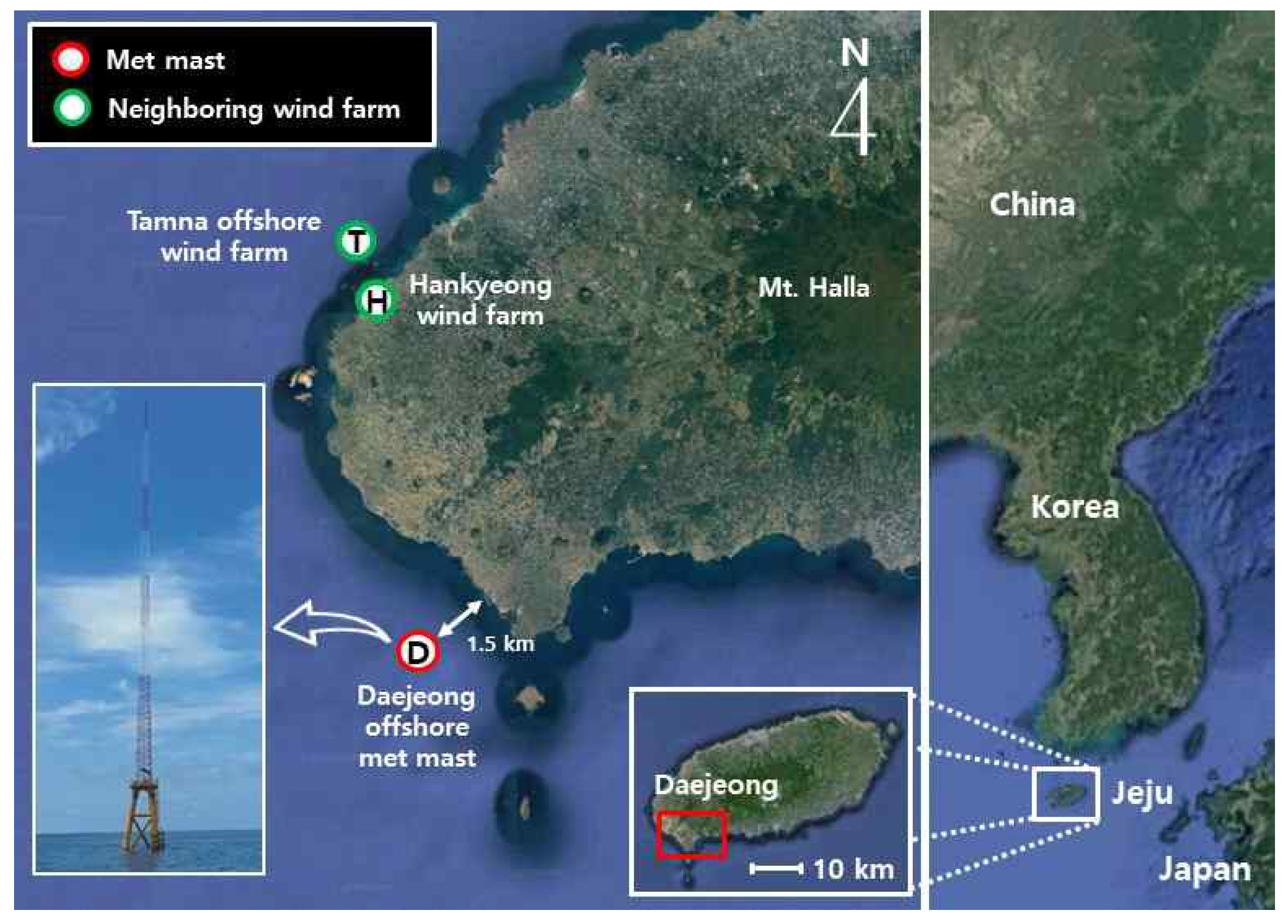
2.1. Daejong Site and Meteorological Mast Description

This study predicted the weather of the Daejeong site, located southwest of Jeju Island, South Korea (Figure 1), using the proposed method and the existing WRF method. Jeju Island is an island located south of the Korean Peninsula. It has 1950 m high Mt. Halla at its center and abundant wind resources throughout the region. The predicted wind speed was compared with the measured data of the met-mast installed at a position 1.5 km away from the Daejeong coast. The met-mast is a 111.5 m high lattice type with a jacket-type substructure. The data measured from the Thies first class anemometer and wind vane installed at a 94 m height were also used.

Table 1. Specifications of wind sensors of the met-mast.

Items	Wind Sensors
	Anemometer	Wind Vane
Model	Thies First class	Thies First class
Measurement range	0–75 m/s	0–360°
Accuracy	0.2 m/s	1.5°
Stating threshold	0.3 m/s	0.2 m/s
Operating temperature	−50–+80 °C	−50–+80 °C
Heights	99 m, 94 m, 88 m, 80 m, 60 m, 20 m	94 m, 88 m, 80 m, 60 m
Tower location	33.19° N, 126.28° E

shows the detailed specifications of these wind sensors.

2.2. Atmospheric–Ocean Coupled Model (WRF-OML)

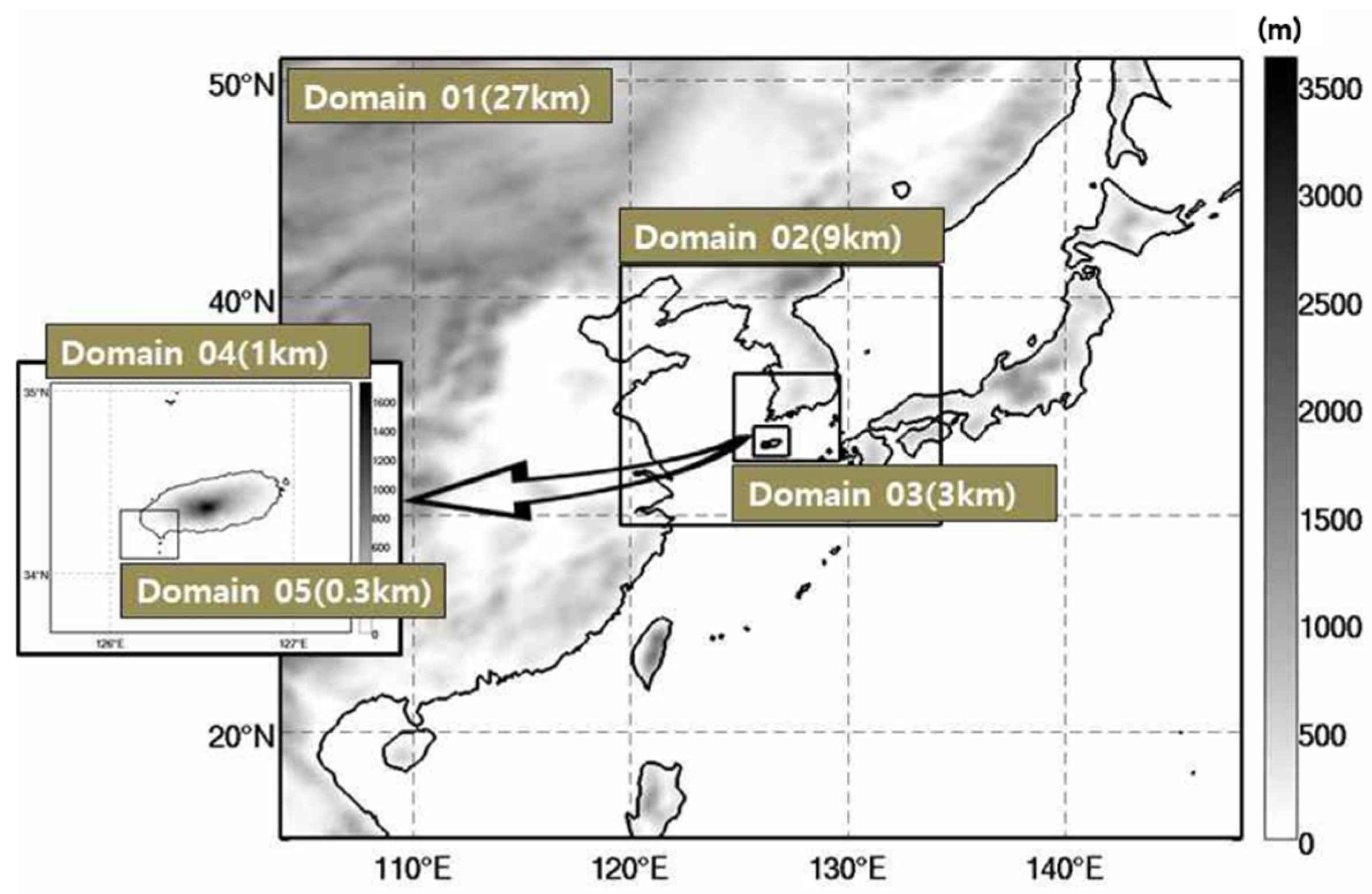
2.2.1. Atmospheric Model (WRF)

In this study, the advanced research WRF (ARW) core of the WRF model (ver. 3.9.1.1) of the National Center for Atmospheric Research (NCAR) was used for atmosphere components of the coupled model [14].

Figure 2 shows the study area, which consisted of five spatial resolution domains based on the southwest coast of Jeju Island.

The model was configured with five two-way nested domains of 27–9–3–1–0.3 km horizontal resolution, with 151 × 151 (Domains 01–04) and 88 × 88 (Domain 05) horizontal grids. A total number of 30 vertical sigma layers were used. The simulation time was set to 48 h for all five domains.

Table 2. WRF physics schemes used in this study.

Variable	Physics Scheme
Microphysics	WDM 6 scheme
Planetary boundary layer	Meller–Yamada–Janjic scheme
Surface layer	Monin–Obulkhov (Janjic) scheme
Land surface	Noah-MP land-surface model
Longwave radiation	RRTM scheme
Shortwave radiation	Dudhia scheme

shows the physics scheme constructed in the WRF model. The cloud physics process used the WRF Double Moment 6-class (WDM 6) scheme [14] and the planetary boundary layer parameterization used the Mellor–Yamada–Janjic scheme (MYJ) [15]. The surface layer parameterization used the Monin–Obukhov scheme [16] and the ground model used the Noah-multiparameterization (Noah-MP) land-surface model [17]. Long-wave radiation and short-wave radiation used the Rapid Radiative Transfer Model (RRTM) parameterization method [18] and Dudhia scheme [19], respectively.

Global forecast system (GFS) data provided by the National Centers for Environmental Prediction (NCEP) were used as the initial and boundary data. The GFS data had a horizontal resolution of 0.5° × 0.5°, with 26 vertical layers. These data provided meteorological information, such as wind, atmospheric pressure, relative humidity and air temperature.

2.2.2. Ocean Mixed Layer Model (OML)

OML, which is a vertically well-mixed layer, plays an important role in determining the exchange of kinetic and thermal energy in the air–sea interface. The upper ocean is usually mixed by ocean current shear-induced turbulent mixing, which is determined by the wind stress and ocean stability; thereby, possibly causing changes in the sea surface temperature. Sea surface temperature changes with the intensity of ocean mixing, which in turn affects the heat flux at the air–sea interface, affecting the atmospheric system [20,21,22,23].

Figure 3 shows the OML model used in this study, which was a one-dimensional model based on Pollard et al. [24] that only considered vertical mixing while ignoring the advection term of the ocean. In this model, wind stress, sensible heat flux, and latent heat flux acted as external forces, which can be expressed using the following equations:

$$\tau =\rho C_D{V}_{10}{}^2,$$

(1)

where $\tau$ is the wind stress, which cools the surface layer by vertical mixing, $\rho$ is the air density, $C_D$ is the drag coefficient, and $V_{10}$ is the wind speed at a height of 10 m. The drag coefficient is related to the roughness length of the surface layer. A fixed roughness length was used on land based on the characteristics of the terrain, whereas a flexible roughness length was used at sea as a function of the wind speed at 10 m under the assumption of a fully developed wave [25,26]:

$$H=\rho C_p{V}_{10}\theta ,$$

(2)

where $H$ is the sensible heat flux determined by the temperature difference between the atmosphere and ocean, $C_p$ is the specific heat of air at constant pressure, $V_{10}$ is the wind speed, and θ is the potential temperature.

$$E=\rho C_E{V}_{10}\Delta q,$$

(3)

where $E$ is the latent heat flux, which is determined by the specific humidity difference between the atmosphere and ocean surface, $C_E$ is the bulk transfer coefficient for water vapor, and $\Delta q$ is the specific humidity difference. The wind stress, the sensible heat flux, and the latent heat flux affected the SST diurnal variation.

In this study, the HYCOM SST data were used to calculate the initial mixed layer depth (MLD), as follows:

$$D=Z- {\left(\frac{2\left(T_{s}Z-H_c\right)}{T}\right)}^{\frac{1}{2}},$$

(4)

where $D$ is the MLD (m) of the ocean, $T_s$ is the upper layer seawater temperature (K), $H_c$ is the upper layer ocean heat contents (Jm⁻²), and $T$ is the water temperature lapse rate (0.2 Km⁻¹) at a water depth of less than 100 m. $Z$ is the minimum depth considered during the calculation of ocean heat contents, which was 100 m for this study.

RTG SST data include only one value of sea surface temperature condition per day, which is not 3D structure, and hence there is no sea surface temperature diurnal variation, while HYCOM SST data have the 3D structure of ocean temperature and its diurnal variation. Figure 4 shows an example of the spatial distribution of RTG SST and HYCOM SST. Figure 4a presents the RTG SST, with the finest spatial resolution of 1/12° (approximately 8 km), where a too high SST was found in the circle of the figure that is the SST close to the equator. On the other hand, the HYCOM SST with the finest spatial resolution of 1/20° (approximately 5 km) is represented in Figure 4b, where a reasonable SST was obtained in the circle of the figure.

OML and WRF were not coupled models using couplers in this study. In the WRF model, we chose a simple ocean mixed layer model as a physics option. To perform OML, SST, initial MLD (mixed layer depth), and rate of sea temperature were required. MLD and rate of sea temperature have the same value for all oceans. Related codes of the WRF model were modified to adjust the values to the studied site. The 2D SST field came out after the 1D calculations in the ocean model, which was transferred to the atmospheric model. Updates were performed once a day, when the model was run. Only SST was transferred from OML to WRF model during coupling.

3. Results

Using the WRF and WRF-OML models, a 48-h meteorological prediction was performed once a day for a year (1 August 2015–31 July 2016), after the SST was updated and reinitialized. Since a 24-h forecast generally gives high accuracy with a short period of time and a 72-h forecast provides low accuracy with a long period, a 48-h forecast was chosen for this study. The results were compared with the met-mast data from the same period. The data used were the wind data at a height of 94 m, which was the hub height. The measurement data were compared with the prediction data of the two models to verify their reliabilities. The recovery rate of the measurement data was 100% (8784 data), while that of the model data was 76.8% for the two models due to the missing GFS model data from the global model, which were required as the initial input data for the regional WRF model. The filtered observation data were used to make one-on-one comparisons between the prediction data of the two models and the observation data.

Table 3. Number of observation data and model data points.

Period	Number of Data Point
	Met-Mast	Filtered	WRF (Recovery Rate (%))	WRF-OML (Recovery Rate (%))
August 2015	744	696	1392 (0.93) (93.5)	1392 (0.93) (93.5)
September 2015	720	384	768 (0.53) (53.3)	768 (0.53) (53.3)
October 2015	744	624	1248 (0.84) (83.9)	1248 (0.84) (83.9)
November 2015	720	696	1392 (0.97) (96.7)	1392 (0.97) (96.7)
December 2015	744	504	1008 (0.68) (67.7)	1008 (0.68) (67.7)
January 2016	744	648	1296 (0.87) (87.1)	1296 (0.87) (87.1)
February 2016	696	672	1344 (0.97) (96.6)	1344 (0.97) (96.6)
March 2016	744	696	1392 (0.94) (93.5)	1392 (0.94) (93.5)
April 2016	720	504	1008 (0.70) (70.0)	1008 (0.70) (70.0)
May 2016	744	240	480 (0.32) (32.3)	480 (0.32) (32.3)
June 2016	720	600	1200 (0.83) (83.3)	1200 (0.83) (83.3)
July 2016	744	480	960 (0.65) (64.5)	960 (0.65) (64.5)
Sum (Recovery Rate (%))	8784 (100.0)	6744 (76.8)	13,488 (76.8)	13,488 (76.8)

lists the 6744 observation data, which are 8784 h within one year multiplied by the recovery rate of 76.8%, and 13,488 predicted model data. The amount of simulated data was twice as much as that of the observation data, because a 48-h duration was used for prediction.

To compare the wind values predicted by the models with those of the met-mast observation data, it was necessary to perform calibration to convert the 10 m prediction data of the models into the prediction data at a height of 94 m, where the actual observation was performed. The power law method was used for this calibration, and the Deacon equation (Equation (5)) was used for the height calibration [27,28]:

$$\frac{U\left(Z\right)}{U\left(Z_a\right)}={\left(\frac{Z_a}{Z}\right)}^{\alpha },$$

(5)

where $Z$ and $U\left(Z\right)$ are the height (m) and the wind speed at Z (m/s), respectively. $Z_a$ and $U\left(Z_a\right)$ are the height (m) and wind speed at $Z_a$ height (m/s), respectively. $\alpha$ is the wind shear exponent. According to the Deacon equation, the wind shear exponent is determined by the terrain change (geometric mean height based on the measurement point) and roughness, as shown in Equation (6) [28]:

$$\begin{array}{l}\alpha =a+b\ln \left[U\left(Z_a\right)\right],\\ a=\frac{1}{\ln \left(\frac{Z_g}{Z_0}\right)}+\frac{0.088}{1-0.088\ln \left(\frac{Z_a}{10}\right)},\\ b=-\frac{0.088}{1-0.088\ln \left(\frac{Z_a}{10}\right)},\end{array}$$

(6)

where $Z_g$ is the geometric mean height (m), $Z_0$ is the roughness, and $Z_a$ is the wind speed measurement height (m).

4. Discussion

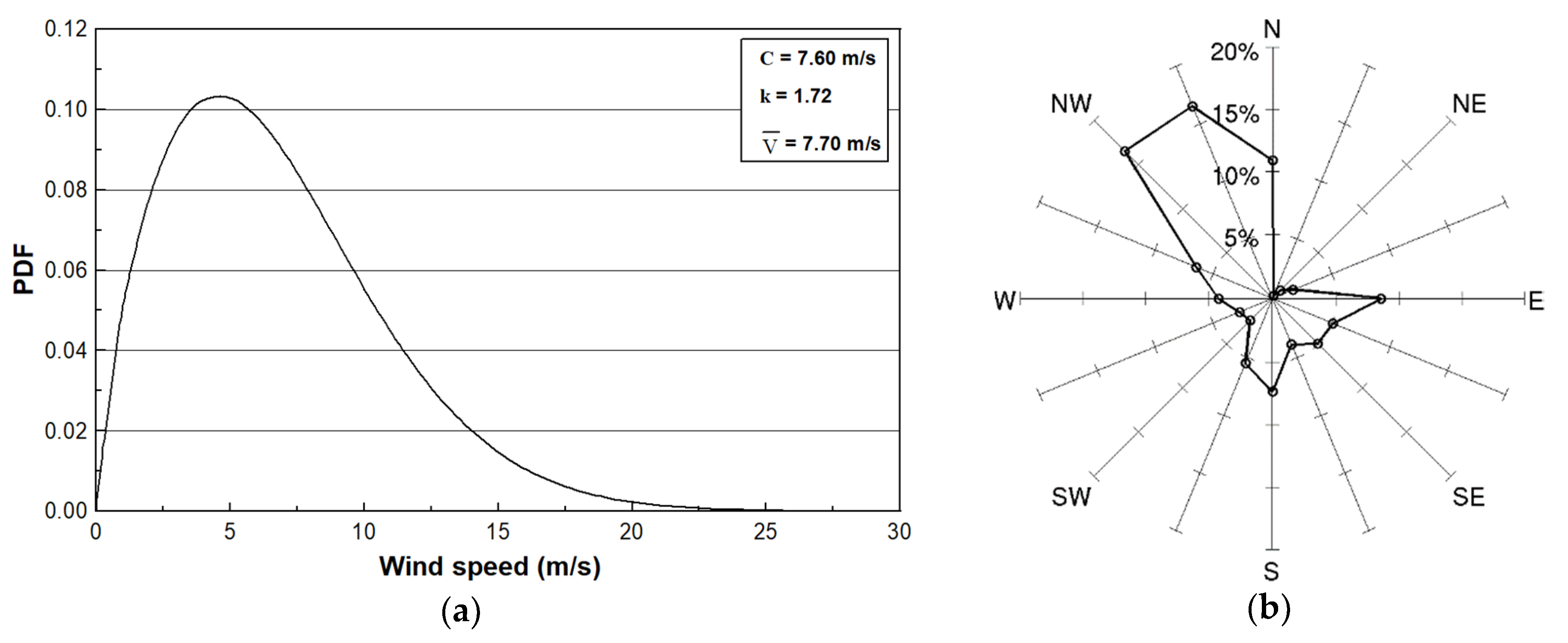
4.1. Basic Wind Resource Assessment

The Weibull distribution is commonly used as the wind speed frequency distribution for calculating the potential wind energy and mean wind speed. This plays an important role for the design of a wind farm. The Weibull distribution can be expressed as a probability density function (PDF), as shown in Equation (7):

$$PDF=\frac{k}{c}{\left(\frac{v}{c}\right)}^{k-1}\exp [-(\frac{v}{c}{)}^k],$$

(7)

The Weibull distribution consists of two parameters, which are c and k. c is a scale factor with a unit of m/s, which is used in determining the wind speed. k is the dimensionless shape factor that determines the geometry of the distribution curve. The Weibull distribution using wind speed data varies depending on the estimation method. Of the several methods, the maximum likelihood estimation method was used in this study.

Figure 5a shows the Weibull distribution at the 94 m hub height. Wind speed between 4 and 6 m/s exhibited the highest frequency. For a year, the mean wind speed was 7.70 m/s, c was 7.60 m/s, and k was 1.72. For these results, 8784 hourly data points observed by the met-mast from 1 August 2015 to 31 July 2016 were used.

Figure 5b shows that the wind rose according to the wind direction frequency in 16 directions. The northwesterly wind and north-northwesterly wind were the main wind directions. The wind frequency from the west-northwesterly wind to the northerly wind was 51.4%, indicating the influence of the continental high pressure dominant in the Korean Peninsula during winter. Other than the northwesterly winds, the southerly wind (6.8%) and easterly wind (7.6%) exhibited relatively meaningful proportions, which is due to the influence of the oceanic air mass in summer and the periodic air pressure pattern generated around Jeju Island in spring and autumn.

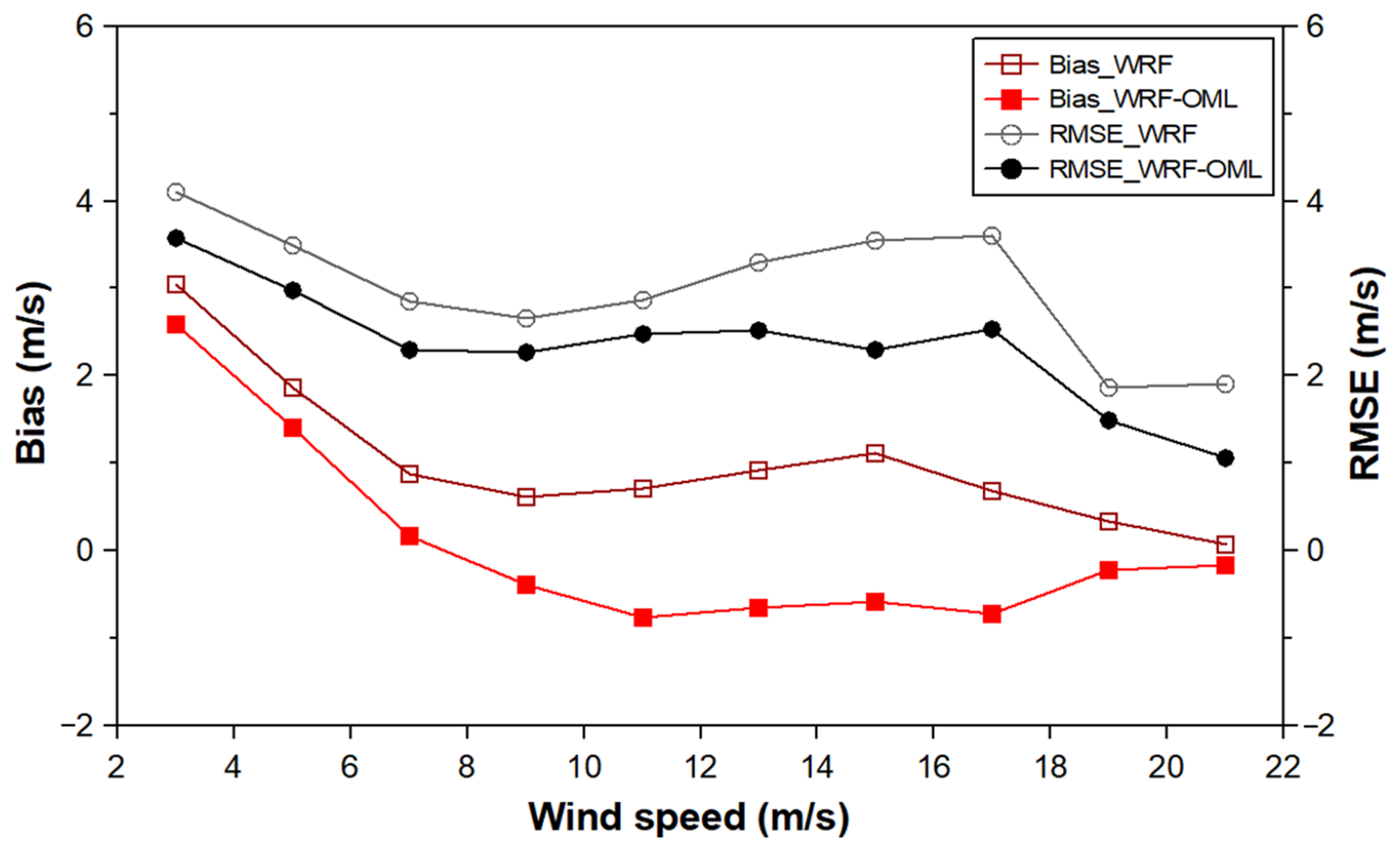
4.2. Wind Speed Prediction Results of WRF and WRF-OML Models at the Hub Height

Statistical methods were used to quantitatively determine the differences in the prediction accuracies of the wind speed and energy production between the two models. The bias and root mean square error (RMSE) were calculated as shown in Equations (8) and (9), respectively:

$$Bias=\frac{1}{N}{{\displaystyle \sum }}_{t=1}^N\left(F_t-A_t\right),$$

(8)

$$RMSE=\sqrt{\frac{{{\displaystyle \sum }}_{t=1}^N{\left(F_t-A_t\right)}^2}{N}},$$

(9)

where $F_t$ is the predicted value and $A_t$ is the observed value.

The 8784 observations were used for the basic wind resource assessment, while the 6744 filtered data points were processed in the two models. As one-on-one correspondence was required to compare the prediction data of each model with the observation data and to compare the model performances, the observation data of the same time were filtered and used. Then, the two predicted wind speeds at the same hour were averaged and compared with the observations at the same hour as predictions.

Figure 6 presents the scatter plots of the simulated results of two models. The bias between the prediction and observation data was 1.09 m/s for the WRF model and −0.07 m/s for the WRF-OML model. The RMSE of the WRF model was 2.88 m/s while that of the WRF-OML model was 2.45 m/s. The coefficient of determination, R², was 0.6716 for the WRF model and 0.6721 for the WRF-OML model. Namely, the WRF-OML model exhibited smaller values for the bias and RMSE.

Figure 7 shows the bias and RMSE for each wind speed. The WRF-OML model exhibited smaller values than the WRF model until 20 m/s. As for the bias, WRF-OML exhibited a better performance in all sections until 20 m/s, even though both models showed overestimation in low wind speed sections. In both models, large errors occurred in the low wind speed sections, i.e., less than 4 m/s. Larger RMSE values were observed in the WRF model than in the WRF-OML model. While the WRF-OML model exhibited stable prediction between 6 and 16 m/s, the WRF model showed more prominent differences.

Figure 8 shows the bias and RMSE according to the prediction time. For the bias, the error repeatedly increased and decreased from the beginning of the prediction time, with increased fluctuations after 42 h. The WRF-OML model exhibited an error 1.02 m/s lower, on average, than the WRF model. In the case of RMSE, the error also increased as the prediction time increased. The WRF-OML model exhibited an average 0.43 m/s lower error than the WRF model. The error of the WRF model increased but the WRF-OML model exhibited smaller error fluctuations immediately after the operation of the models, indicating the effect of reflecting the OML model.

Figure 9 displays the seasonal bias and RMSE for wind speed. The WRF-OML model clearly had less seasonal bias and RMSE than the WRF model. The average values during all the seasons for the two errors were the same as those in Figure 6. The seasonal variation was not found much for the two errors.

Table 4. Monthly mean wind speed from the observation data and from the models for the filtered data.

Period	Met-Mast	WRF		WRF-OML
	Wind Speed (m/s)	Wind Speed (m/s)	Ratio (%)	Wind Speed (m/s)	Ratio (%)
August 2015	5.60	6.52	116.4	5.71	102.0
September 2015	7.45	8.57	115.0	7.48	100.4
October 2015	7.12	7.88	110.7	6.92	97.2
November 2015	8.06	9.56	118.6	8.34	103.5
December 2015	9.16	11.00	120.1	9.41	102.7
January 2016	10.09	11.64	115.4	10.24	101.5
February 2016	10.62	11.68	110.0	10.32	97.2
March 2016	8.07	9.63	119.3	7.95	98.5
April 2016	6.53	7.65	117.2	6.53	100.0
May 2016	8.85	9.36	105.8	8.13	91.9
June 2016	5.91	6.11	103.4	5.45	92.2
July 2016	6.71	7.14	106.4	6.44	96.0
Total	7.85	8.89	113.2	7.74	98.6

lists the wind speed measured by the met-mast and predicted by the two models. At a mean wind of 7.85 m/s, as observed by the met-mast, the mean wind speed prediction of the WRF model was 8.89 m/s, indicating an overestimation of 13.2%, whereas that of the WRF-OML model was 7.74 m/s, indicating an underestimation of 1.4%. That is, the WRF-OML model showed better prediction performance than the WRF model, with a monthly mean wind speed of 0.93 m/s and an error rate of 11.8%. Throughout the entire observation period, the WRF-OML model exhibited data closer to the observation measurements, whereas the WRF model exhibited overestimation.

4.3. Energy Production Prediction Results of WRF and WRF-OML Models

The wind speed prediction validity of the WRF and WRF-OML models was analyzed using the Weibull distribution. Figure 10 presents the Weibull distribution functions of the met-mast and the two models as a power curve of the 5.56 MW wind generator of Company A, which was used in this study. The WRF-OML model and met-mast exhibited similar values for the mean wind speed and scale and shape factors of the Weibull distribution. On the other hand, the WRF model estimated higher wind speeds than that of the met-mast and WRF-OML model.

The annual energy production (AEP) of the two models was estimated by applying the power curve of the 5.56 MW wind generator of Company A to the Daejeong offshore site. The results were then compared with the AEP estimated from the met-mast data. The wind generator used had a cut-in wind speed of 3.5 m/s, cut-out wind speed of 25 m/s, rated wind speed of 13 m/s, and rated power of 5.56 MW.

As shown in Equation (10), AEP can be calculated using the Weibull distribution through the measurement data and power curve provided by the wind generator manufacturer:

$$\mathrm{AEP}={{\displaystyle \sum }}_{i=1}^N\left(P\left(V_i\right)\times f\left(V_i\right)\times 8760\right),$$

(10)

where AEP is the annual power generation (kWh), P(V) is the generated power of the wind speed V (kW), and f(V) is the occurrence probability of the wind speed V. The sum of the generated power calculated for each wind speed from the cut-in wind to cut-out wind speed was the annual energy production. In the above equation, 8760 is the number of one-hour intervals in one year. Since the measurement period in this study was a leap year, 8784 h were used.

Figure 11 shows the RMSE and bias results for WRF and WRF-OML based on the prediction time. Although both models maintained a similar trend for the bias, the WRF model exhibited overestimation with an average error of 289 kW, while the WRF-OML model exhibited a smaller average error of up to −87 kW. The bias of the WRF model was consistently positive, which agreed with its tendency for wind speed overestimation. The bias of the WRF-OML model fluctuated around zero, with small error values. For the RMSE, both models maintained a similar trend, except during 26–32 and 36–40 h. The average error of 1.26 MW of the WRF-OML model was smaller than that of 1.36 MW of the WRF model.

Table 5. Monthly power production from the met-mast observation data and from the prediction data of the models.

Period	Met-Mast	WRF		WRF-OML
	Power Production (kW)	Power Production (kW)	Ratio (%)	Power Production (kW)	Ratio (%)
August 2015	774.29	1062.87	137.3	724.95	93.6
September 2015	831.77	959.53	115.4	784.92	94.4
October 2015	1271.69	1386.24	109.0	1102.76	86.7
November 2015	1729.84	2196.71	127.0	1749.55	101.1
December 2015	1623.35	1954.01	120.4	1643.49	101.2
January 2016	2306.01	2586.51	112.2	2402.99	104.2
February 2016	2502.44	2784.71	111.3	2406.58	96.2
March 2016	1769.73	2058.19	116.3	1611.97	91.1
April 2016	866.58	1102.16	127.2	801.11	92.4
May 2016	716.08	730.40	102.0	551.74	77.1
June 2016	837.99	823.95	98.3	616.03	73.5
July 2016	855.70	900.81	105.3	733.62	85.7
Total	16,085.47	18,546.09	115.3	15,129.71	94.1

shows the energy production calculated from the met-mast and the two models. Comparing the monthly energy production results, the WRF-OML model exhibited highly similar results to those of the met-mast observation data. On the other hand, the WRF model showed overestimated outputs during the entire period except for June. Comparing the annual energy production results with met-mast data, the WRF model showed 15.3% overestimation, while the WRF-OML model exhibited 5.9% underestimation. For both models, the section with high wind speed prediction reliability conformed to that with high output prediction reliability, indicating the direct relationship between the prediction accuracy of the wind speed and energy production. Consequently, it was found that the wind speeds and outputs predicted by the WRF-OML model were 11.8% and 9.4%, respectively, closer to the actual values than those predicted by the WRF model.

5. Conclusions

This study compared the atmospheric model (WRF) and the atmosphere–ocean model (WRF-OML) in predicting the wind speed and wind power produced at sea. The WRF-OML model coupled the atmospheric model and ocean mixed layer model (OML), and applied the hybrid coordinate ocean model (HYCOM) to the three-dimensional ocean water temperature data.

The observation data from the Daejeong offshore meteorological mast (met-mast) were used to verify the predicted wind speed at sea and the energy production data. The prediction data of the two models were compared with the observation data at a 94 m height. The results were as follows:

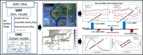
• Comparing the wind speed prediction, the average bias was 1.09 for the WRF model and −0.07 for the WRF-OML model. The root mean square error (RMSE) was 2.88 for the WRF model and 2.45 for the WRF-OML model. Thus, the WRF-OML model has a better prediction performance than the WRF model;
• Both models showed overestimation tendencies at low wind speeds (less than 4 m/s) and provided relatively stable prediction between 6 and 16 m/s, with increased error as the prediction time increased;
• Comparing the energy production prediction by prediction time, the average error between the WRF-OML and WRF models was 202 kW for the bias and 107 kW for the RMSE, thus confirming a better performance from the WRF-OML model;
• In comparison to the met-mast data, the WRF model overestimated the wind speed and annual energy production by 13.2% and 15.3%, respectively, while the WRF-OML model underestimated them by 1.4% and 5.9%, respectively. Consequently, the wind speed and energy prediction reliability of the WRF-OML model were 11.8% and 9.4% higher than that of the WRF model;
• Since the WRF-OML model was only validated for the Daejeong offshore site in this work, it is necessary to investigate further for other offshore sites with various conditions to further validate the model.

The results of this study show the significance of using the atmosphere–ocean mixed layer coupled model, which considers the seawater mixing process by tides, upwelling, strong wind, and the subsequent changes in the sea surface temperature (SST), for the accurate prediction of offshore wind power production, which is more difficult than the prediction of offshore wind speed.

References

1. Chancham, C.; Waewsak, J.; Gagnon, Y. Offshore wind resource assessment and wind power plant optimization in the Gulf of Thailand. Energy 2017, 139, 706–731. [Google Scholar] [CrossRef]
2. Wang, Y.H.; Walter, R.K.; White, C.; Farr, H.; Ruttenberg, B.I. Assessment of surface wind datasets for estimating offshore wind energy along the Central California Coast. Renew. Energy 2019, 133, 343–353. [Google Scholar] [CrossRef]
3. Carvalho, D.; Rocha, A.; Gómez-Gesteira, M.; Santos, C. A sensitivity study of the WRF model in wind simulation for an area of high wind energy. Environ. Model. Softw. 2012, 33, 23–34. [Google Scholar] [CrossRef] [Green Version]
4. Cavalho, D.; Rocha, A.; Gómez-Gesteira, M.; Santos, C.S. Sensitivity of the WRF model wind simulation and wind energy production estimates to planetary boundary layer parameterizations for onshore and offshore area in the Iberian Peninsula. Appl. Energy 2014, 135, 234–246. [Google Scholar] [CrossRef]
5. Mattar, C.; Borvarán, D. Offshore wind powers simulation by using WRF in the central coast of Chile. Renew. Energy 2016, 94, 22–31. [Google Scholar] [CrossRef]
6. Di, Z.; Ao, J.; Duan, Q.; Wang, J.; Gong, W.; Shen, C.; Gan, Y.; Liu, Z. Improving WRF model turbine-height wind-speed forecasting using a surrogate-based automatic optimization method. Atmos. Res. 2019, 226, 1–16. [Google Scholar] [CrossRef]
7. Park, R.S.; Cho, Y.K.; Choi, B.J.; Song, C.H. Implications of sea surface temperature deviations in the prediction of wind and precipitable water over the Yellow Sea. J. Geophys. Res. 2011, 116, D17. [Google Scholar] [CrossRef] [Green Version]
8. Schade, L.R.; Emanuel, K.A. The ocean’s effect on the intensity of tropical cyclones: Results from a simple cou- pled atmosphere-ocean model. J. Atmos. Sci. 1999, 56, 642–651. [Google Scholar] [CrossRef] [Green Version]
9. Kawai, Y.; Otsuka, K.; Kawamura, H. Study on diurnal sea surface warming and a local atmospheric circulation over Mutsu Bay. J. Meteorol. Soc. Jpn. 2006, 84, 725–744. [Google Scholar] [CrossRef] [Green Version]
10. Dai, A.; Trenberth, K.E. The diurnal cycle and its depiction in the community climate system model. J. Clim. 2003, 17, 930–951. [Google Scholar] [CrossRef]
11. Noh, Y.; Lee, E.; Kim, D.H.; Hong, S.Y.; Kim, M.J.; Ou, M.L. Prediction of the diurnal warming of sea surface temperature using an atmosphere-ocean mixed layer coupled model. J. Geophys. Res. 2011, 116, C11. [Google Scholar] [CrossRef] [Green Version]
12. Chang, S.W.; Anthes, R.A. The mutual response of the tropical cyclone and the ocean. J. Phys. Oceanogr. 1979, 9, 128–135. [Google Scholar] [CrossRef] [Green Version]
13. Lee, C.Y.; Chen, S.S. Symmetric and asymmetric structures of hurricane boundary layer in coupled atmosphere-wave-ocean models and observations. J. Atmos. Sci. 2012, 69, 3576–3594. [Google Scholar] [CrossRef]
14. NCAR. ARW Modeling System V3.9 User’s Guide; National Center for Atmospheric Research: Boulder, CO, USA, 2017. [Google Scholar]
15. Mellor, G.L.; Yamada, T. Development of a turbulence closure model for geophysical fluid problems. Rev. Geophys. Space Phys. 1982, 20, 851–875. [Google Scholar] [CrossRef] [Green Version]
16. Jiménez, P.A.; Dudhia, J.; González-Rouco, J.F.; Navarro, J.; Montávez, J.P.; García-Bustamante, E. A revised scheme for the WRF surface layer formulation. Mon. Weather Rev. 2012, 140, 898–918. [Google Scholar] [CrossRef] [Green Version]
17. Chen, F.; Dudhia, J. Coupling an advanced land surface–hydrology model with the Penn State-NCAR MM5 Modeling system. Part II: Preliminary model validation. Mon. Weather Rev. 2001, 129, 587–604. [Google Scholar] [CrossRef]
18. Mlawer, E.J.; Taubman, S.J.; Brown, P.D.; Iacono, M.J.; Clough, S.A. Radiative transfer for inhomogeneous atmospheres: RRTM, a validated correlated-k model for the longwave. J. Geophys. Res. Atmos. 1997, 102, 16663–16682. [Google Scholar] [CrossRef] [Green Version]
19. Dudhia, J. Numerical study of convection observed during the winter monsoon experiment using a mesoscale two-dimensional model. J. Atmos. Sci. 1989, 46, 3077–3107. [Google Scholar] [CrossRef]
20. Mohan, G.M.; Srinivas, C.V.; Naidu, C.V.; Baskaran, R.; Venkatraman, B. Real-time numerical simulation of tropical cyclone Nilam with WRF: Experiments with different initial conditions, 3D-Var and ocean mixed layer model. Nat. Hazards 2015, 77, 597–624. [Google Scholar] [CrossRef]
21. Price, J.F.; Weler, R.A.; Pinkel, R. Diurnal cycling: Observations and models of the upper ocean response to diurnal heating, cooling, and wind mixing. J. Geophys. Res. 1986, 91, 8411–8427. [Google Scholar] [CrossRef] [Green Version]
22. Price, J.F. Upper ocean response to a hurricane. J. Phys. Oceanogr. 1981, 11, 153–175. [Google Scholar] [CrossRef] [Green Version]
23. Wu, C.C.; Tu, W.T.; Pun, I.F.; Lin, I.I.; Peng, M.S. Tropical cyclone-ocean interaction in Typhoon Megi (2010)—A synergy study based on ITOP observations and atmosphere-ocean coupled model simulations. J. Geophys. Res. 2016, 121, 153–167. [Google Scholar] [CrossRef]
24. Pollard, R.T.; Rhines, P.B.; Thompson, R.Y. The deepening of the wind-mixed layer. Geophys. Fluid Dyn. 1973, 4, 381–404. [Google Scholar] [CrossRef]
25. Manwell, J.F.; Rogers, A.L.; McGowan, J.G.; Bailey, B.H. An offshore wind resource assessment study for New England. Renew. Energy 2002, 27, 175–187. [Google Scholar] [CrossRef]
26. Powell, M.D.; Vickery, P.J.; Reinhold, T.A. Reduced drag coefficient for high wind speed in tropical cyclones. Nature 2003, 422, 279–283. [Google Scholar] [CrossRef] [PubMed]
27. Valsaraj, K.T.; Melvin, E.M. Elements of Environmental Engineering Thermodynamics and Kinetics, 3rd ed.; CRC Press: Boca Raton, FL, USA, 2009; pp. 454–456. ISBN 978-1-4200-7820-6. [Google Scholar]
28. Cheang, E.H.; Moon, C.J.; Jeong, M.S.; Jo, K.P.; Park, G.Y. The study for calculating the geometric average height of Deacon equation suitable to the domestic wind correction methodology. J. Korean Sol. Energy Soc. 2010, 30, 9–14. [Google Scholar]
Figure 1. Location of Jeju Island and measurement site in Daejeong.
Energies 13 00254 g001
Figure 2. Configuration of the two-way nested domains of the weather research forecasting (WRF) model. Sizes of the domains (from left to right) are 27 km, 9 km, 3 km, 1 km and 0.3 km. Darkness represents the topography.
Energies 13 00254 g002
Figure 3. Schematics of the one-dimensional ocean mixed layer (OML) model used for the WRF model.
Energies 13 00254 g003
Figure 4. (a) Spatial distributions of real time global sea surface temperature (RTG SST) used in the original WRF model and (b) spatial distributions of hybrid coordinate ocean model sea surface temperature (HYCOM SST) used in the WRF-OML model at 00 UTC 1 July 2016.
Energies 13 00254 g004
Figure 5. Configuration of (a) Weibull distribution and (b) wind speed (at 94-m height) of the Daejeong offshore site.
Energies 13 00254 g005
Figure 6. Scatter plots of simulated results using (a) the WRF model and (b) the WRF-OML model (wind speed at 94 m height) with observations at Deajeong tower.
Energies 13 00254 g006
Figure 7. Bias and root mean square error (RMSE) of simulated results using WRF and WRF-OML (wind speed at 94-m height) models with wind speed.
Energies 13 00254 g007
Figure 8. Bias and RMSE of simulated results using WRF and WRF-OML (wind speed at 94-m height) models with prediction time.
Energies 13 00254 g008
Figure 9. Bias and RMSE of the simulated results using the WRF and WRF-OML (wind speed at 94-m height) models with seasons. Spring is March to May, summer is June to August, autumn is September to November, and winter is December to February.
Energies 13 00254 g009
Figure 10. Weibull distribution of the met-mast, WRF, WRF-OML, and power curve of the wind turbine used in the study. V ¯ f i l t e r e d is mean wind speed using the filtered measurement data, Pm is measured power, and Pr means rated power.
Energies 13 00254 g010
Figure 11. Bias and RMSE of simulated results using WRF and WRF-OML (power production at 94-m height) models with prediction time.
Energies 13 00254 g011