New Intelligent Control Strategy Hybrid Grey–RCMAC Algorithm for Ocean Wave Power Generation Systems

Abstract

In this article, the characteristics of the wave energy converter are considered and a novel dynamic controller (NDC) for a permanent magnet synchronous generator (PMSG) is proposed for Wells turbine applications. The proposed NDC includes a recursive cerebellum model articulation controller (RCMAC) with a grey predictor and innovative particle swarm optimization (IPSO). IPSO is developed to adjust the learning speed and improve learning capability. Based on the supervised learning method, online adjustment law of RCMAC parameters is derived to ensure the system’s stability. The NDC scheme is designed to maintain a supply–demand balance between intermittent power generation and grid power supply. The proposed NDC exhibits an improved power regulation and dynamic performance of the wave energy system under various operation conditions. Furthermore, better results are obtained when the RCMAC is used with the grey predictive model method.

1. Introduction

Owing to the increasing energy demand and global effects of the climate change, the use of clean energy sources, such as wind, solar, tidal, and microhydropower, has become important. Wave energy has been considered as a potential alternative energy source owing to its richness and pollutionless property [1,2,3].

The ocean provides a promising but challenging source for renewable energy development. To simplify assumptions such as monochromatic wave environments and linear fluid dynamics, the optimal energy extraction control for the wave energy converter (WEC) has been defined [4]. Although information about wide-ranging WEC performance is limited, the wave energy industry is fast developing. Therefore, the economic efficiency of WEC systems (WECS) is far from rivaled, and the use of intelligent control systems to improve capacity term varies widely [5]. A well-designed and properly controlled Wells turbine electromechanical drive can operate at low air velocity to reduce the average generated power, but this performance is not desirable [6]. Recently, the sliding mode control (SMC) theory based on the variable structure system has been a good choice especially for the wave energy conversion systems [7,8].

The grey prediction model is a nonlinear extrapolation forecasting method, developed in the 1980s, which is characterized by strong practicability, flexible modeling, and high forecasting accuracy, and requires less data than other methods. Thus, grey prediction models have been diffusely used in various fields of natural sciences and social sciences. To overcome the shortcomings associated with neural networks (NNs), a cerebellar model articulation controller (CMAC) was proposed by Albus in 1975 to identify and control complex dynamical systems [9]. CMAC has the advantages of learning quickly, strong recapitulation ability, and simple hardware implementation [10,11].

A traditional CMAC is a perceptual associative memory network with incomplete connections and strong local generalization abilities that uses constant binary or triangular functions. However, it has the drawback that its derived information is not retained. To obtain the derivative information of the input and output variables, the CMAC network used a differentiable Gaussian acceptance field basis function and analyzed its convergence [12]. The advantages of CMAC networks over NNs have been well recorded in many applications [13,14]. However, the combination of grey theory and the CMAC algorithm can improve the learning ability, effectiveness, and robustness of predictions.

Particle swarm optimization (PSO) was first developed by Kennedy and Eberhart in 1995 [15,16]. The method is inspired by mimicking animal social behaviors, such as fish schooling, bird flocking, and swarm theory. Genetic algorithm (GA) is also a population-based and self-adaptive optimization tool and is effective in optimizing difficult multidimensional discontinuous problems in a variety of fields [17]. Unlike GA, PSO has memorial ability to keep the knowledge of good solutions, and can be retained by all particles, while the previous knowledge is not memorized in GA. In population-based optimization algorithms, there is a necessity for new algorithms that can improve the performance of the existing algorithms while enhancing particle swarm optimization with time varying acceleration coefficients to perform the parameter tuning approach, which has an important capability in improving the performance of the PSO.

Herein, an IPSO algorithm is introduced to determine optimal parameters of recurrent CMAC (RCMAC) controllers for back-to-back converters of the PMSG. To improve the better online dynamic characteristics, IPSO is used to find the best learning rate of RCMAC. The results were compared with conventional CMAC and recurrent fuzzy neural network (RFNN) method and their robustness was verified. As a result, the novel dynamic controller could obtain good dynamic performance of WECS and the maximum power extraction. The overall simulation model was built for such systems in various cases through the power systems computer aided design (PSCAD)/electromagnetic transient design and control (EMTDC) platform.

2. Modeling of the Studied System

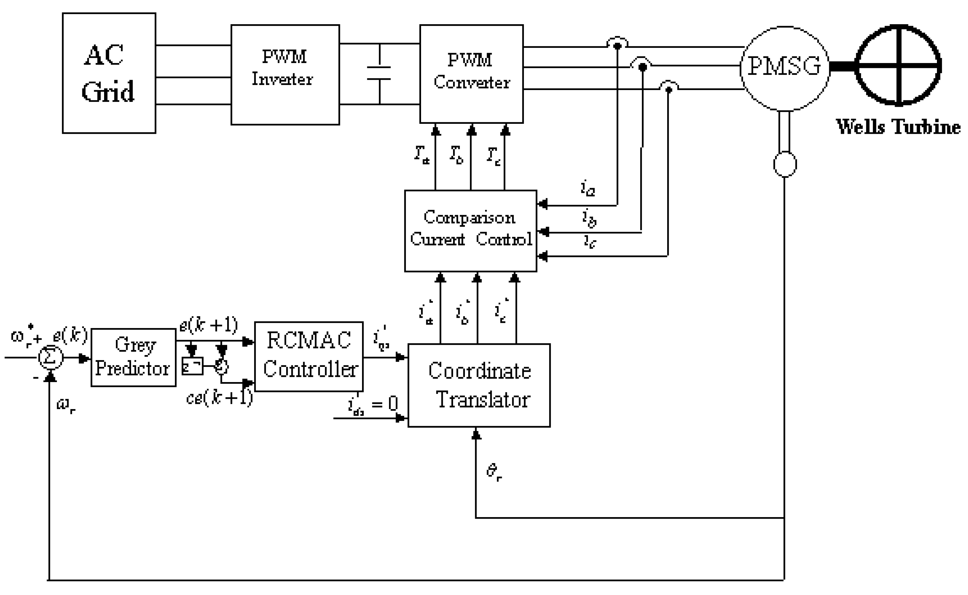
2.1. Structure of the System

The schematic of a PMSG-based Wells turbine system is shown in Figure 1. The PMSG is driven by the Wells turbine to deliver maximum power to the AC grid. A designed AC/DC converter then converts the AC power generated by the PMSG into an adjustable DC power. An effective method of DC link voltage control based on a Grey–RCMAC control system is proposed for wave period variations of the turbine or load changes, controlling the electromagnetic torque of a PMSG driven using the variable speed Wells turbine; the effects of different speed variation forms are considered.

2.2. Wells Turbine Modeling

The captured mechanical torque ($T_m$), torque coefficient ($C_t$), and turbine blade incidence angle ($\alpha$) from the wave energy of the Wells turbine can be described by [18].

$$Tm=k{C}_t(V_A^2+V_B^2),$$

(1)

$$C_t=C_8+\frac{C_1{\alpha }^3-C_2{\alpha }^2+C_3\alpha -C_4}{C_5{\alpha }^2+C_6\alpha -C_7},$$

(2)

$$\alpha ={\tan }^{-1}\left(\frac{V_A}{V_B}\right),$$

(3)

where V_A and V_B are the axial velocity and blade tip speed, respectively, k is the Wells turbine coefficient, C₁–C₈ are constants, and $\alpha$ is the arctangent of the V_A to V_B ratio.

2.3. PMSG Modeling

The PMSG machine model can be described in the rotor rotating d-q reference frame as [19,20].

$$\begin{gathered} v_q=R{i}_q+p{\lambda }_q+{\omega }_s{\lambda }_d \\ {v}_d=R{i}_d+p{\lambda }_d-{\omega }_s{\lambda }_q \end{gathered}$$

(4)

and

$$\begin{gathered} {\lambda }_q=L_q{i}_q \\ {\lambda }_d=L_d{i}_d+L_{md}{I}_{fd} \end{gathered}$$

(5)

$${\omega }_s=P{\omega }_r$$

(6)

where

• $v_d,v_q=$d, q axis stator voltages
• $i_d,i_q=$d, q axis stator currents
• $L_d,L_q=$d, q axis stator inductances
• ${\lambda }_d,{\lambda }_q=$d, q axis stator flux linkages
• $R=$ stator resistance
• ${\omega }_s=$ inverter frequency
• $I_{fd}=$ equivalent d-axis magnetizing current
• $L_{md}=$d-axis mutual inductance

The electrical torque ($T_e$) for a three-phase PMSG can be defined as follows [21]:

$$T_e=3P[L_{md}{I}_{fd}{i}_q+\left(L_d-L_q\right)i_d{i}_q]/2=\frac{P_e}{{\omega }_e}=\frac{2}{P}\frac{P_e}{{\omega }_r}$$

(7)

Therefore, the mechanical dynamic equation of the PMSG can be expressed as follows:

$$J\frac{d{\omega }_r}{dt}=T_m-B{\omega }_r-T_e,$$

(8)

where ${\omega }_e$ is the electrical angular frequency, P is the poles number, J is the generator’s coefficient of inertia, and B is the generator’s coefficient of friction.

3. Design of Maximum Power Point Tracking (MPPT) Controller Based on RCMAC with Grey Forecasting

From grey theory, the random process is the amount of grey that varies within a certain range of amplitude and certain time zone, and treats the random process as a grey process. Notwithstanding the use of statistical rules, grey prediction makes correlation analysis by identifying the degree of difference between the development factors of system factors, and generates and processes the original data to find the law of system variation, generates a data sequence with strong regularity, and then establishes the corresponding differential equation model, thereby predicting the future development of things [22].

3.1. The Online Grey Dynamic Prediction Model

The two data modeling methods of the grey system are accumulated generating operation (AGO) and inverse AGO (IAGO). The order of AGO and IAGO is determined by the number of grey differential equations and grey variables of the model, respectively. The grey model GM(d,v) is a dynamic behavior containing a group of differential equations, where d and v represent the order and variation of the differential equation, respectively. Generation time exponentially increases with an increase in d and v; however, large d and v values cannot ensure improved forecast accuracy [23,24]. The GM(1,1) is a predictive method for predicting existing data and is widely used in prediction applications in grey systems.

If the original data is listed as $Y^{(0)}=\left[y^{(0)}(1),y^{(0)}(2),\dots ,y^{(0)}(n)\right]$, performing AGO processing, defined as an AGO queue, $Y^{(1)}=\left[y^{(1)}(1),y^{(1)}(2),\dots ,y^{(1)}(n)\right]$ is derived as follows:

$$y^{(1)}(k)={\displaystyle \sum _{m=1}^k{y}^{(0)}}(m),k=1,2,\cdots n$$

(9)

From $Y^{(1)}$, the first-order differential equation of the GM(1,1) model is as follows:

$$\frac{d{y}^{(1)}}{dt}+a{y}^{(1)}=u,$$

(10)

where a and u are the developing coefficient and grey input variable, respectively.

Then discretized

$${\widehat{y}}^{(1)}(k+1)=(y^{(0)}(1)-\frac{u}{a})e^{-ak}+\frac{u}{a},k=1,2,\cdots n$$

(11)

By least-square method, they can be expressed as follows:

$$\left[\begin{array}{c}a\\ u\end{array}\right]={(A^{T}A)}^{-1}{A}^{T}Z,$$

(12)

where

$$A=\left[\begin{array}{cc}-\frac{1}{2}(y^{(1)}(1)+y^{(1)}(2))& 1\\ -\frac{1}{2}(y^{(1)}(2)+y^{(1)}(3)& 1\\ \cdots & \cdots \\ -\frac{1}{2}(y^{(1)}(n-1)+y^{(1)}(n))& 1\end{array}\right],$$

(13)

$Z={\left[y^{(0)}(2),y^{(0)}(3),\dots ,y^{(0)}(n)\right]}^T$, and ${\widehat{y}}^{(1)}(k+1)$ is the predicted value of $y^{(1)}(k+1)$ at time k + 1.

With the developed GM(1,1) model, we know that only non-negative data can be used for it. Deng [23] added sequence bias to the proposed scheme; therefore, all elements can be added to avoid negative effects. The grey system uses current error $e(k)$ to forecast the future error $e(k+1)$ of the next RCMAC controller, as shown in Figure 1. Furthermore, the error and change of error can be defined as $e(k)={\omega }_r^{*}(k)-{\omega }_r(k)$ and $ce(k)=e(k)-e(k-1)$, respectively.

3.2. Recurrent CMAC Controller

The CMAC has incompletely connected and overlapping receivers similar to an associative memory network [14]. In comparison with a multilayer perceptron using back-propagation algorithm, the CMAC has the advantages of fast learning speed, strong versatility, and convenient calculation, and has been widely used in closed loop control for complex dynamic systems.

The traditional CMAC uses a local constant binary receiving field basis function. The disadvantages of this method are that output is constant in each quantization state and derivative information is not retained. Therefore, a dynamic CMAC, with a delay self-recurrent unit added to the relevant storage space and RCMAC [9,25], is introduced herein.

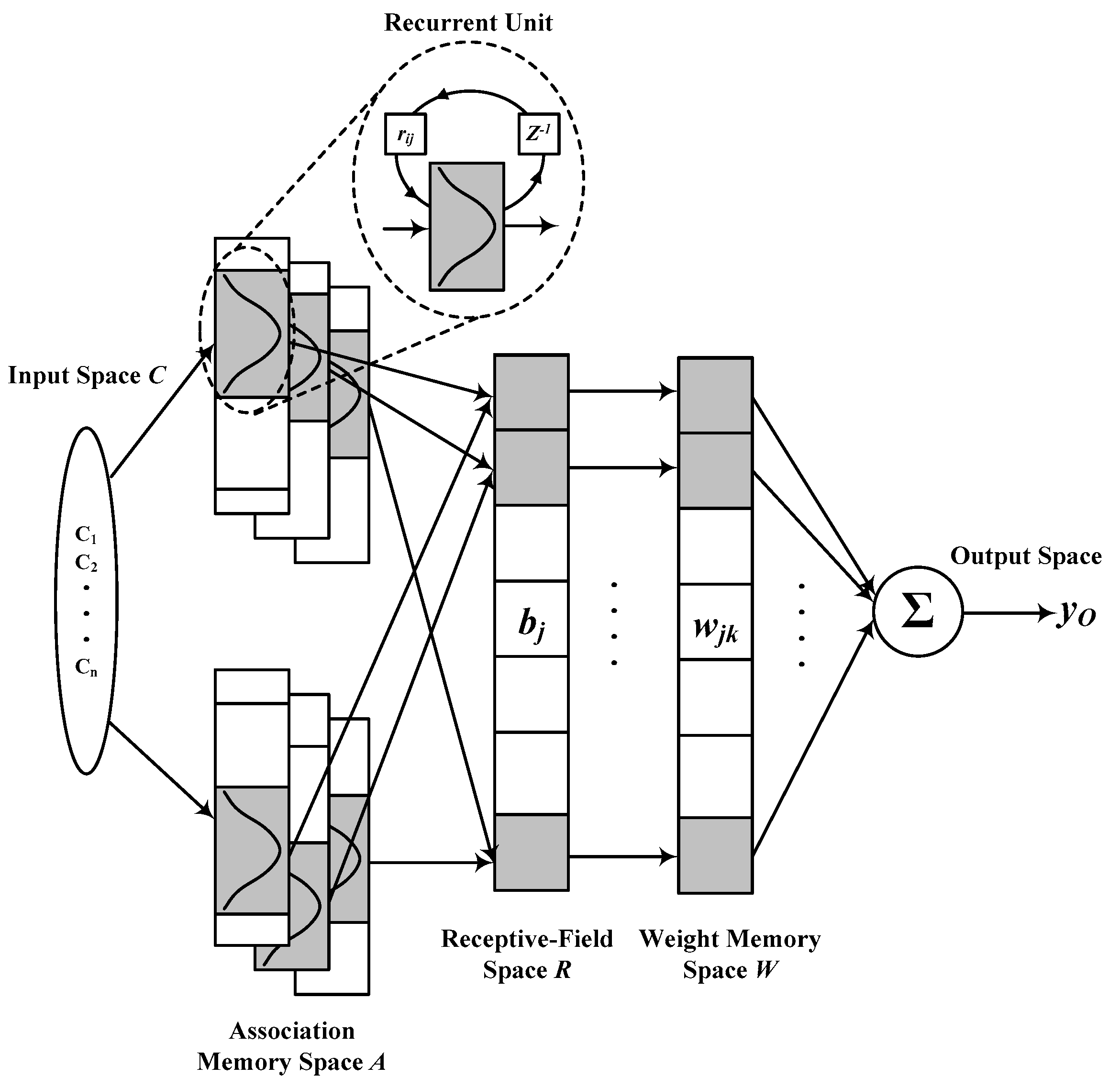
3.2.1. RCMAC Structure

Figure 2 shows a proposed RCMAC, where z⁻¹ denotes a time delay. This RCMAC comprises input, association memory, receptive field, weight memory, and output spaces. Signal propagation for each layer is introduced as follows:

• Input Layer: For a given C = [$e(k+1)$, $ce(k+1)$], each input variable c_i can be quantized into discrete reference states.
• Association Memory Layer: To effectively assign each input state in learning. Herein, the Gaussian function (receptive field basis function) is built into the hypercube block as Equation (14). In the bell-shaped manner of the Gaussian function, when the discontinuous input state is closer to the center of a certain cube, the output is more affected by the cube, and vice versa. The farther the impact is, the smaller it is.

$$\begin{gathered} {\psi }_{ij}=\exp \frac{-{(c_{ri}-L_{ij})}^2}{S_{ij}^2} \\ \mathrm{for}j=1,2,\dots n{\mathrm{and}}_{}i=1,2,\dots n \end{gathered}$$

(14)

${\psi }_{ij}$ denotes the receptive field basis function for the jth hypercube block of the ith input, $c_{ri}$,with location parameter, $L_{ij}$, and scale parameter, $S_{ij}$. Additionally, this block’s input can be expressed as follows:

$$c_{ri}^{}(t)=c_i^{}(t)+r_{ij}{\psi }_{ij}^{}(t-1)$$

(15)

where $r_{ij}$ is the recurrent gain and ${\psi }_{ij}^{}(t-1)$ indicates the value of ${\psi }_{ij}^{}(t)$ through a time delay. Clearly, this block’s input contains memory term ${\psi }_{ij}^{}(t-1)$, which stores the network’s past information and presents dynamic mapping. Each hypercube block in this space has three tunable parameters:$L_{ij}$, $S_{ij}$, and $r_{ij}$.

• Receptive Field Layer: The multidimensional receptive field function is expressed as follows:

  $$b_j={\Pi }_{i=1}^N{\psi }_{ij}=exp\left[-\left({\displaystyle {\sum }_{i=1}^N\frac{{(c_{ri}-L_{ij})}^2}{S_{ij}^2}}\right)\right]$$

  (16)
• Weight Memory Layer: This space specifies adjustable weights of the receptive field layer results as follows:

  $$\begin{gathered} w_k={\left[w_{1k},w_{2k},\cdots w_{N_{R}k}\right]}^T \\ \mathrm{for}k=1,2,\dots ,m \end{gathered}$$

  (17)
• Output Layer: The output of RCMAC mathematic form and also the control effort of the proposed controller is obtained as follows:

  $$i_{qs}^{*}=y_0=w_k^{T}b={\displaystyle {\sum }_{j=1}^{N_R}{w}_{jk}}\exp \left[-\left({\displaystyle {\sum }_{i=1}^N\frac{{(c_{ri}-L_{ij})}^2}{S_{ij}^2}}\right)\right]$$

  (18)

3.2.2. RCMAC Learning Algorithm

Herein, a RCMAC is proposed and parameters are updated by the back-propagation algorithm. The adaptive adjustment in gradient descent setting imposes additional stability and increases learning speed [26,27]. To describe the RCMAC online learning method, the cost function E_c is defined as follows:

$$E_c=\frac{1}{2}{\left({\omega }_r^{*}-{\omega }_r\right)}^2=\frac{1}{2}{e}_L^2,$$

(19)

where ${\omega }_r^{*}$ and ${\omega }_r$ denote the generator’s speed reference and speed feedback, respectively, and $e_L$ is the tracking error.

The error term which will be propagated is obtained as follows:

$${\delta }_o^{}=-\frac{\partial E_c}{\partial y_0}=-\frac{\partial E_c}{\partial e_L}\frac{\partial e_L}{\partial {\omega }_r}\frac{\partial {\omega }_r}{\partial y_0}=e_L\frac{\partial {\omega }_r}{\partial y_0}$$

(20)

Then, the adjusted weight $w_{jk}^{}$ is updated by the amount

$$\Delta w_{jk}^{}=-\frac{\partial E_c}{\partial w_{jk}^{}}=\left[-\frac{\partial E_c}{\partial y_o^{}}\right]\left(\frac{\partial y_0}{\partial w_{jk}}\right)={\delta }_o^{}{b}_j^{}$$

(21)

Therefore, the weight $w_{jk}^{}$ is updated to

$$w_{jk}^{}\left(t+1\right)=w_{jk}^{}\left(t\right)+{\eta }_w\Delta w_{jk}^{},$$

(22)

where ${\eta }_w$ is the learning rate for the weight.

Multiplication operation is performed in this layer. The adaptive rules for $L_{ij}$ and $S_{ij}$ are expressed. First, the error term is computed as follows:

$${\zeta }_j^{}=-\frac{\partial E_c}{\partial b_j^{}}=\left[-\frac{\partial E_c}{\partial y_o^{}}\right]\left(\frac{\partial y_0^{}}{\partial b_j^{}}\right)={\delta }_0^{}{w}_{jk}^{},$$

(23)

where k indicates the regulation associated with the jth node in layer 2. Then, the adaptive law for $L_{ij}$ and $S_{ij}$ are computed as follows:

$$\Delta L_{ij}=-\frac{\partial E_c}{\partial L_{ij}}=\left[-\frac{\partial E_c}{\partial y_0^{}}\frac{\partial y_0^{}}{\partial {\psi }_{ij}^{}}\right]\left(\frac{{\psi }_{ij}}{\partial L_{ij}}\right)={\rho }_{ij}^{}\frac{2\left(c_{ri}^{}-L_{ij}\right)}{{\left(S_{ij}\right)}^2}$$

(24)

and

$$\Delta S_{ij}=-\frac{\partial E_c}{\partial S_{ij}}=\left[-\frac{\partial E_c}{\partial y_0^{}}\frac{\partial y_0^{}}{\partial {\psi }_{ij}^{}}\right]\left(\frac{\partial {\psi }_{ij}}{\partial S_{ij}}\right)={\rho }_{ij}^{}\frac{2{\left(c_{ri}^{}-L_{ij}\right)}^2}{{\left(S_{ij}\right)}^3}$$

(25)

Then, the location and scale parameters of the receptive field layer are given as follows:

$$L_{ij}\left(t+1\right)=L_{ij}\left(t\right)+{\eta }_L\Delta L_{ij}$$

(26)

and

$$S_{ij}\left(t+1\right)=S_{ij}\left(t\right)+{\eta }_S\Delta S_{ij}$$

(27)

The factors ${\eta }_L$ and ${\eta }_S$ are the learning rate for the location and scale parameter of the Gaussian function, respectively, and an adequate condition for the asymptotic stability of the original system is also given. Convergence of the RCMAC learning process is guaranteed when the learning rate is applied to regulate the optimum weight value. The ${\eta }_w$, ${\eta }_L$, and ${\eta }_S$ are optimized using the IPSO algorithm. With a RCMAC controller, the hybrid Grey–RCMAC controller with IPSO can increase system stability.

3.3. Adjust Learning Rates with IPSO

To further enhance the online learning ability of RCMAC, a hybrid time-varying IPSO algorithm based on a genetic algorithm is proposed to adjust learning rate ${\eta }_w$, ${\eta }_L$, and ${\eta }_S$. When the new IPSO runs, each particle of the PSO will adjust its position according to its own and adjacent particle’s solving experience, which includes the current position, current velocity, and previous best position of itself and adjacent particles [28].

R₁ and R₂ are two pseudo-random sequences used to simulate the randomness of the algorithm. For each m, $R{c}_i^m$ and $pb{t}_i^m$ are the current positions and current best position of oneself, respectively. The velocity updating law is shown in Equation (28). Besides, the inertia weight $w$ is set to 0 and IPSO can reduce parameter settings. Acceleration coefficients $c_1$ and $c_2$ can be modified using Equations (29) and (30). These settings are known as time-varying acceleration coefficients and are expressed as follows [29]:

$$\begin{array}{ll}{\upsilon }_i^m(t+1)=& w{\upsilon }_i^m(t)+c_1\cdot R_1\cdot (pb{t}_i^m-R{c}_i^m(t))\\ & +c_2\cdot R_2\cdot (gb{t}_i^m-R{c}_i^m(t))\end{array}$$

(28)

The time-varying acceleration coefficients are updated using the following formulas:

$$c_1=(c_{1f}-c_{1i})\cdot \frac{t}{t_{\max }}+c_{1i},$$

(29)

$$c_2=(c_{2f}-c_{2i})\cdot \frac{t}{t_{\max }}+c_{2i},$$

(30)

$$R{c}_i^m(t+1)=R{c}_i^m(t)+{\upsilon }_i^m(t+1),$$

(31)

where ${\upsilon }_i^m$ and $R{c}_i^m$ are the current particle velocities and positions, respectively, t_max is the maximum number of iterations, $c_{1i}$ and $c_{2i}$ are the initial parameters settings, and $c_{1f}$ and $c_{2f}$ are the final parameters settings.

Step 1: Define initial conditions

$R{c}_i^m=\left[R{c}_i^1,R{c}_i^2,R{c}_i^3\right]$ for learning rates $({\eta }_w,{\eta }_L,{\eta }_S)$, set the population size P = 12 and particle dimension to d = 3. The problem of optimizing parameters is concerned as a d-dimensional solution space.

Step 2: Initialize the particle’s position and velocity

Initialize all particles and randomly set the position $R{c}_i^m(t)$ and velocities ${\upsilon }_i^m(t)$ of particles. The current position of the initial particle itself is pbt, and the position of the particle group is gbt. $R{c}_i^m(t)$ values are randomly generated as follows:

$$R{c}_i^m(t)~U[{\eta }_{\min }^d,{\eta }_{\max }^d],$$

(32)

where $U[{\eta }_{\min }^d,{\eta }_{\max }^d]$ indicates the results of uniformly distributed random variables, whose ranges exceed the lower bound learning rate ${\eta }_{\min }^{}$ and upper bound rate ${\eta }_{\max }^{}$.

Step 3: Evaluate the fitness of each particle

All particles are fitness functions to determine the fitness and evaluated for each vector $R{c}_i^m(t)$. Herein, choose the appropriate fitness function to calculate the fitness value FIT of each particle.

$$FIT=\frac{1}{0.1+abs({\omega }_r-{\omega }_r^{*})},$$

(33)

where 0.1 is added to the denominator to keep FIT from approaching infinity.

Step 4: Select pbt and gbt

Each particle $R{c}_i^m(t)$ has a memory function to remember its fitness and select the best fitness so far as its $pb{t}_i^m$. Thus, the maximum vector $pb{t}_i^m=[pb{t}_1^m,pb{t}_2^m,\dots pb{t}_p^m]$ of the population is obtained. In addition, during the first iteration, the $R{c}_i^m$ of each particle is set to $pb{t}_i^m$ directly, and the most suitable particle of all pbt values is set to the global best gbt.

Step 5: Verify gbt for updates

IPSO is used to update the velocity and position updating formula for the top-ranking particles of fitness function, whereas the crossover operation of the genetic algorithm is used to update the lower-ranking particles. Position and velocity are then reorganized as follows:

$$R{c}_i^m(t+1)=c_3\cdot rand()\cdot (gb{t}_i^d-R{c}_i^m(t)),$$

(34)

$$\begin{array}{c}{p}_{child1}=\rho p_{pa1}+(1-\rho )p_{pa2}\\ p_{child2}=\rho p_{pa2}+(1-\rho )p_{pa1}\end{array},$$

(35)

$$\begin{array}{c}{v}_{ch1}=\frac{v_{pat1}+v_{pa2}}{\left|v_{pat1}+v_{pa2}\right|}\cdot \left|v_{pa1}\right|\\ v_{c\mathrm{h}2}=\frac{v_{pat1}+v_{pa2}}{\left|v_{pat1}+v_{pa2}\right|}\cdot \left|v_{pa2}\right|\end{array},$$

(36)

where $c_3$ is the acceleration factor, rand () is a random function with a range of [0, 1], $p_{pa}$ and $p_{ch}$ are parent and child generations of position, respectively, and $v_{pa}$ and $v_{ch}$ are parent and child generations of velocity, respectively, and $\rho$ represents the interpolation value between parent and child generation uniform random numbers among 0 and 1.

Step 6: Update velocity and position

Then, the updated velocity of the particle is subjoined to the current position of the particle and updated relative to its own optimal position and global optimal position following Equations (26) and (29).

Step 7: Reach the end condition

Repeat Steps 3–6 until the best adaptation of gbt is worth improving or reaching the set of this generation. The final maximum fitness value $gb{t}_i^m$ is the optimal learning rate of RCMAC.

4. Simulation Results and Discussion

Herein, four cases are used to simulate the dynamic responses of wave generation systems under different power disturbances and grid failures. The performance of Grey–RCMAC with IPSO is compared with that of a conventional RCMAC, CMAC, RFNN controller, and proportional–integral (PI) controller. These methods have been tested in various ways, and Figure 3, Figure 4, Figure 5 and Figure 6 describe the control behavior responses of each controller and

Table 1. Performance comparison of power extraction with five control methods.

Controller	Power Efficiency (%)	Max Error of Torque Coefficient Ct (%)	MPPT Accuracy (%)	Transient Response (s)
Grey–RCMAC	90.9	0.65	0.41	1.65
RCMAC	86.7	10.11	1.12	2.27
CMAC	80.1	15.61	2.29	3.51
RFNN	84.3	14.35	2.19	2.72
PI	77.5	22.65	2.82	4.57

,

Table 2. Comparison results for five methods for the Wells turbine rotational speed change: (a) real power of WECS, (b) reactive power of WECS, and (c) dynamic voltage amplitude response of AC bus on power grid side.

(a) Real Power of Wells Turbine
Controller	Convergence Time (s)	CPU Execution Time	Mean Square Error (10−3)	Accuracy (%)
		(102 s)
Grey–RCMAC	11.99	5.61	4.01	95.99
RCMAC	12.67	5.92	6.21	93.79
CMAC	9.15	4.30	10.73	89.27
RFNN	8.11	3.81	8.52	91.48
PI	13.50	6.34	21.15	78.85
(b) Reactive Power of Wells Turbine
Controller	Convergence Time (s)	CPU Execution Time (102 s)	Mean Square Error (10−2)	Accuracy (%)
Grey–RCMAC	10.83	5.09	4.28	95.72
RCMAC	12.50	5.875	7.15	92.85
CMAC	13.93	6.54	12.11	87.89
RFNN	9.72	4.56	10.95	89.05
PI	11.67	5.48	18.59	81.41
(c) Dynamic Voltage Amplitude Response of AC Bus on Power Grid Side
Controller	Convergence Time (s)	CPU Execution Time (102 s)	Mean Square Error (pu)	Accuracy (%)
Grey–RCMAC	4.33	3.313	0.167	98.33
RCMAC	4.50	3.443	0.835	91.65
CMAC	5.81	4.444	1.161	88.39
RFNN	5.87	4.490	0.677	93.23
PI	N/A	N/A	1.502	85

,

Table 3. Comparison for five methods under the load switching: (a) real power of WECS, (b) reactive power of WECS, and (c) dynamic voltage amplitude response of AC bus on power grid side.

(a) Real Power of Wells Turbine
Controller	Convergence Time (s)	CPU Execution Time (102 s)	Mean Square Error (10−2)	Accuracy (%)
Grey–RCMAC	5.66	4.30	3.080	96.92
RCMAC	7.50	5.07	5.390	94.61
CMAC	6.28	4.77	7.912	92.09
RFNN	8.18	6.21	6.667	93.33
PI	8.00	6.08	9.230	90.77
(b) Reactive Power of Wells Turbine
Controller	Convergence Time (s)	CPU Execution Time (102 s)	Mean Square Error (10−2)	Accuracy (%)
Grey–RCMAC	5.66	4.07	5.001	94.99
RCMAC	7.66	5.51	13.336	86.66
CMAC	7.04	5.06	14.912	85.08
RFNN	6.15	4.67	9.730	90.27
PI	7.83	5.63	21.667	78.33
(c) Dynamic Voltage Amplitude Response of AC Bus on Power Grid Side
Controller	Convergence Time (s)	CPU Execution Time (102 s)	Mean Square Error (10−2)	Accuracy (%)
Grey–RCMAC	6.00	4.56	5.001	94.99
RCMAC	7.66	5.82	8.335	91.66
CMAC	7.16	5.44	10.721	89.28
RFNN	6.74	5.12	7.056	92.94
PI	8.00	6.08	13.333	86.67

and

Table 4. Comparison for five controllers when a fault occurs: (a) real power of WECS, (b) reactive power of WECS, and (c) transient voltage amplitude response of AC bus on power grid side.

(a) Real Power of WECS
Controller	Convergence Time (s)	CPU Execution Time (102 s)	Mean Square Error (10−2)	Accuracy (%)
Grey–RCMAC	2.40	1.82	7.50	92.50
RCMAC	2.65	2.01	15.00	85.00
CMAC	3.11	2.36	16.56	83.44
RFNN	2.45	186	11.91	88.09
PI	3.60	2.73	20.00	80.00
(b) Reactive Power of WECS
Controller	Convergence Time (s)	CPU Execution Time (102 s)	Mean Square Error (10−2)	Accuracy (%)
Grey–RCMAC	2.25	1.71	5.01	94.99
RCMAC	2.75	2.09	11.25	88.75
CMAC	3.71	2.82	13.53	86.47
RFNN	3.04	2.31	8.03	91.97
PI	4.31	3.28	16.25	83.75
(c) Transient Voltage Amplitude Response of AC Bus on Power Grid Side
Controller	Convergence Time (s)	CPU Execution Time (102 s)	Mean Square Error (10−2)	Accuracy (%)
Grey–RCMAC	2.55	1.93	5.00	95.00
RCMAC	2.90	2.20	12.50	87.5
CMAC	3.57	2.71	15.08	84.92
RFNN	2.86	2.17	8.91	91.09
PI	4.52	3.43	18.75	81.25

summarize the relevant characteristics. The method is simulated and analyzed herein, and the parameters of the Wells turbine generator are as follows:

Wells turbine: S_PMSG = 20 MW, 3.75 A, 3000 rpm, J = 1.32 × 10⁻³ Nms², B = 5.78 × 10⁻³ Nm s/rad, V = 15 KV, PF = 0.975, f = 60 Hz, C_dc = 0.6 pu, and T_R = 0.69/33 kV.

Optimal learning rate simulations using IPSO algorithm aims to use PMSG for enhancing the overall dynamic response of proposed wave device integration in case of sudden severe load changes or power network failures [30,31,32].

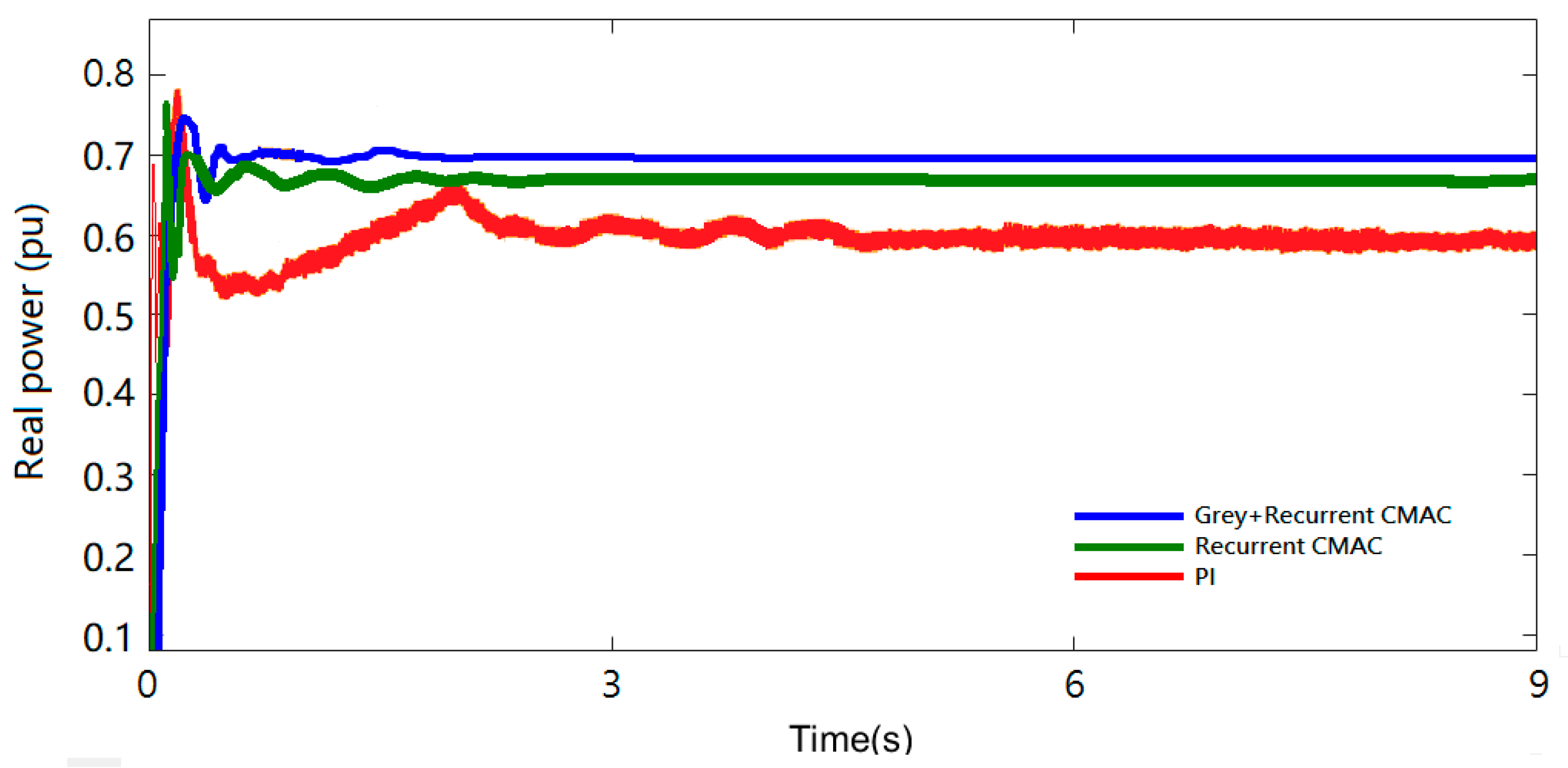
4.1. MPPT System Performance

The time domain simulation of a wave energy system was run with constant load under sufficient ocean waves. WECS output power is shown in Figure 3, which demonstrates that Grey–RCMAC has a smaller transient response, smaller oscillation, and best control response in comparison with the traditional PI controller. The transient response at the beginning clearly shows that the PI controller fluctuates more, whereas the Grey–RCMAC oscillates only slightly. The Grey–RCMAC, RCMAC, and PI controller average powers are 0.7, 0.675, and 0.597 pu, respectively. It can be seen in Figure 3 that the proposed Grey–RCMAC improves by 14.7% more than the PI controller. Table 1 lists the numerical comparison results of more control methods and shows the robustness of the Grey–RCMAC control.

4.2. Wells Turbine Variable Axial Velocities

The Wells turbine rotational speed changes from 15.5 to 4.5 and 4.5 to 12 m/s at 4 and 11 s, respectively. The Wells turbine’s rotor speed response is shown in Figure 4a. The RCMAC-based PMSG’s WECS rotor speed’s return to the steady state response is the fastest, demonstrating that the Grey–RCMAC with IPSO implements better than the RCMAC and PI controllers from the viewpoint of speed perturbation resistance. Figure 4b,c show the performance of three controllers for real and reactive power under the variation of wave speed change, respectively, and illustrate real power variations of the PMSG. The Grey–RCMAC with IPSO control scheme has fast tracking response speed and more stable and better power flow control effect. The disturbance of Grey–RCMAC is smaller than that of RCMAC and PI controllers in power variation. The AC bus voltage of PMSG on the grid side is shown in Figure 4d. When the WECS rotor speed changes, this method can minimize the change in voltage output amplitude and recover to 1.0 pu as soon as possible. On the contrary, Figure 4d shows that among the three methods, the amplitude of the PI controller varies the most when t = 4 and 10 s, the RCMAC amplitude changes the least, followed by recurrent CMAC.

On the other hand, the random characteristics of practical ocean waves produce an oscillation in the pressure drop [7,8]. To investigate the robustness and usefulness of the Grey–RCMAC control scheme, two cases studied are conducted. Figure 5a shows the pressure variation of the studied system. Figure 5b,c illustrate the performance of two controllers for real power and generator speed of the PMSG, respectively, and they randomly change between 0 and 0.7 pu as well as between 0.8 and 1.12 pu. Figure 5d,e plot the dynamic responses of the real power and the generator speed of the PMSG, respectively, and they randomly vary between 0 and 0.6 pu as well as between 0.7 and 1.0 pu. Table 2 summarizes the numerical comparison results of the PI, RFNN, CMAC, RCMAC, and Grey–RCMAC with IPSO controller for Wells turbine speed changes.

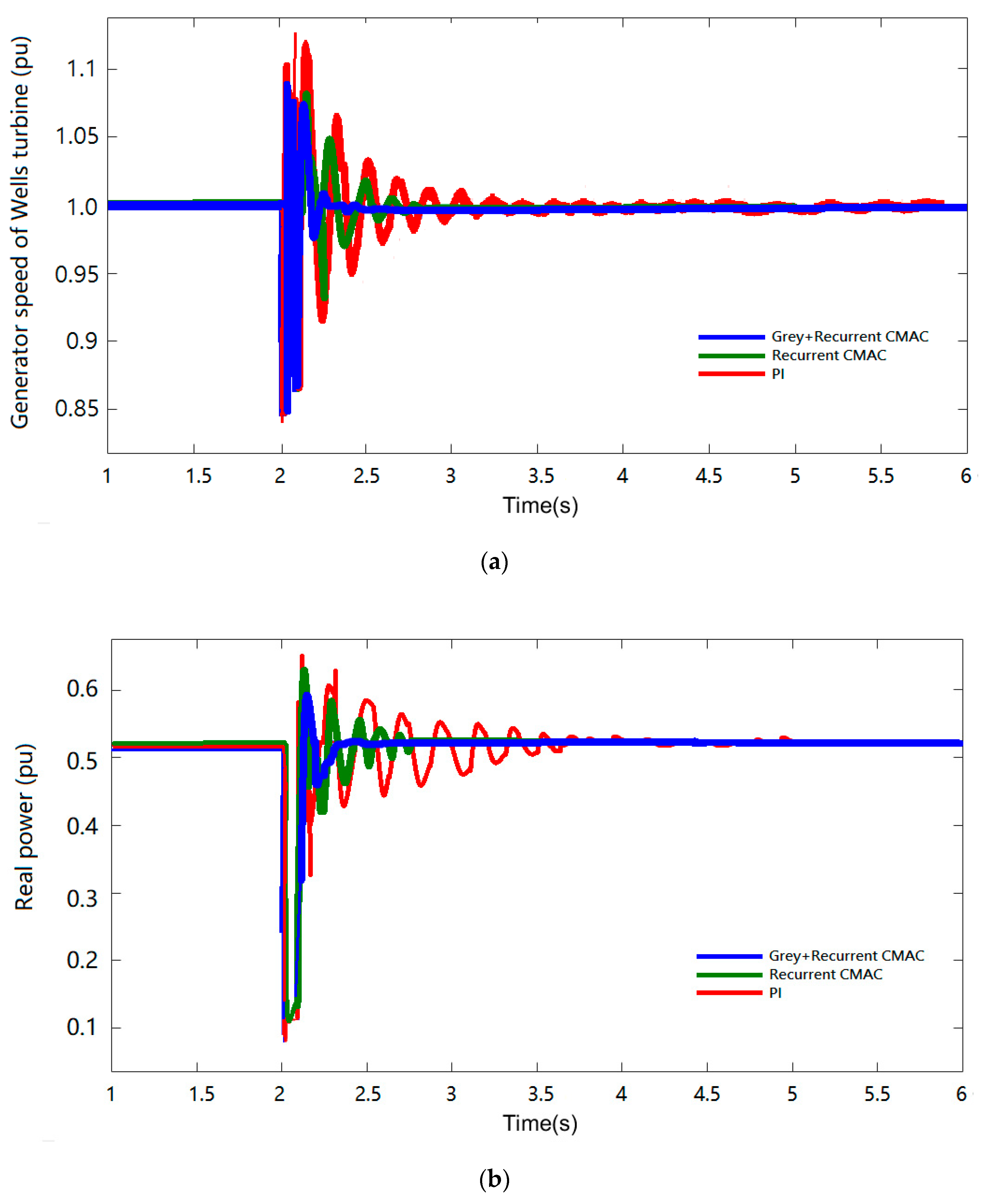
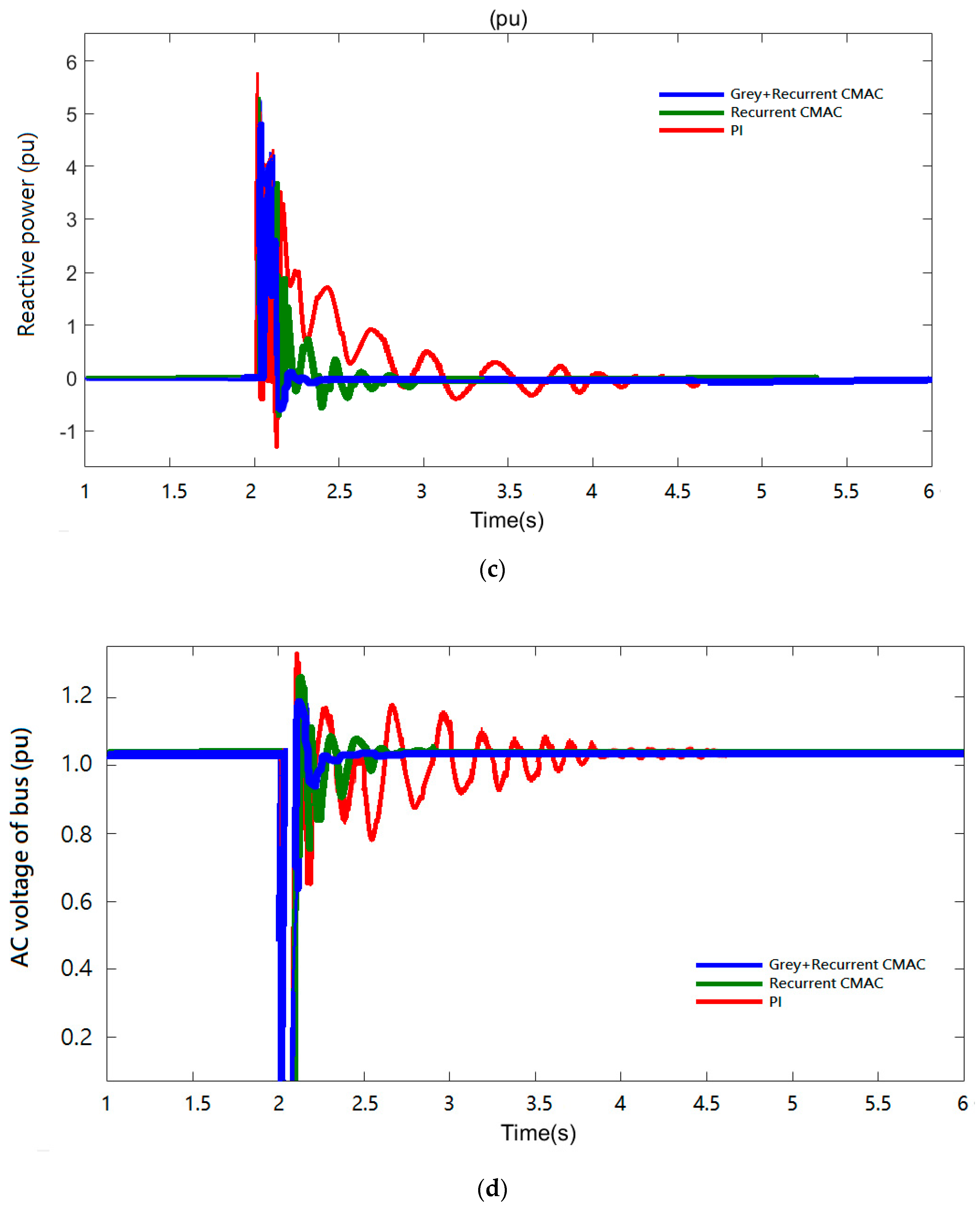
4.3. Dynamic Load Switching

The load changes at t = 5 and 10 s, going from 0.5 to 0.8 and 0.8 to 0.4 pu, respectively. Figure 6a shows the PMSG-based wave power generation system’s rotor speed response. The three methods show the oscillation of rotor speed, wherein the PI controller has the greatest change in rotor amplitude swing, whereas Grey–RCMAC with IPSO technology has the smallest variation in rotor amplitude swing. Small changes for real power response amplitude of the PMSG, as shown in Figure 6b, demonstrate that among the three methods, it is the quickest to return to the steady state. Obviously, using a PI controller or RCMAC, real power variations are larger than those with the proposed controller. Figure 6b,c clearly shows that the power oscillation is very small and can be eliminated quickly by the proposed method. Figure 6d shows the dynamic amplitude performance of the AC bus voltage at the PMSG grid side. As shown in Figure 6d, in comparison with the RCMAC and PI controllers, when using Grey–RCMAC with IPSO, it is easy to observe the maximum overshoot decreases significantly and the AC bus voltage returns to steady state quickly. Simulation results of the PI, RCMAC, and Grey–RCMAC with IPSO controller for load changes are summarized in Table 3. From the abovementioned results, it is concluded that the proposed control scheme has satisfactory dynamic performance with respect to the other methods.

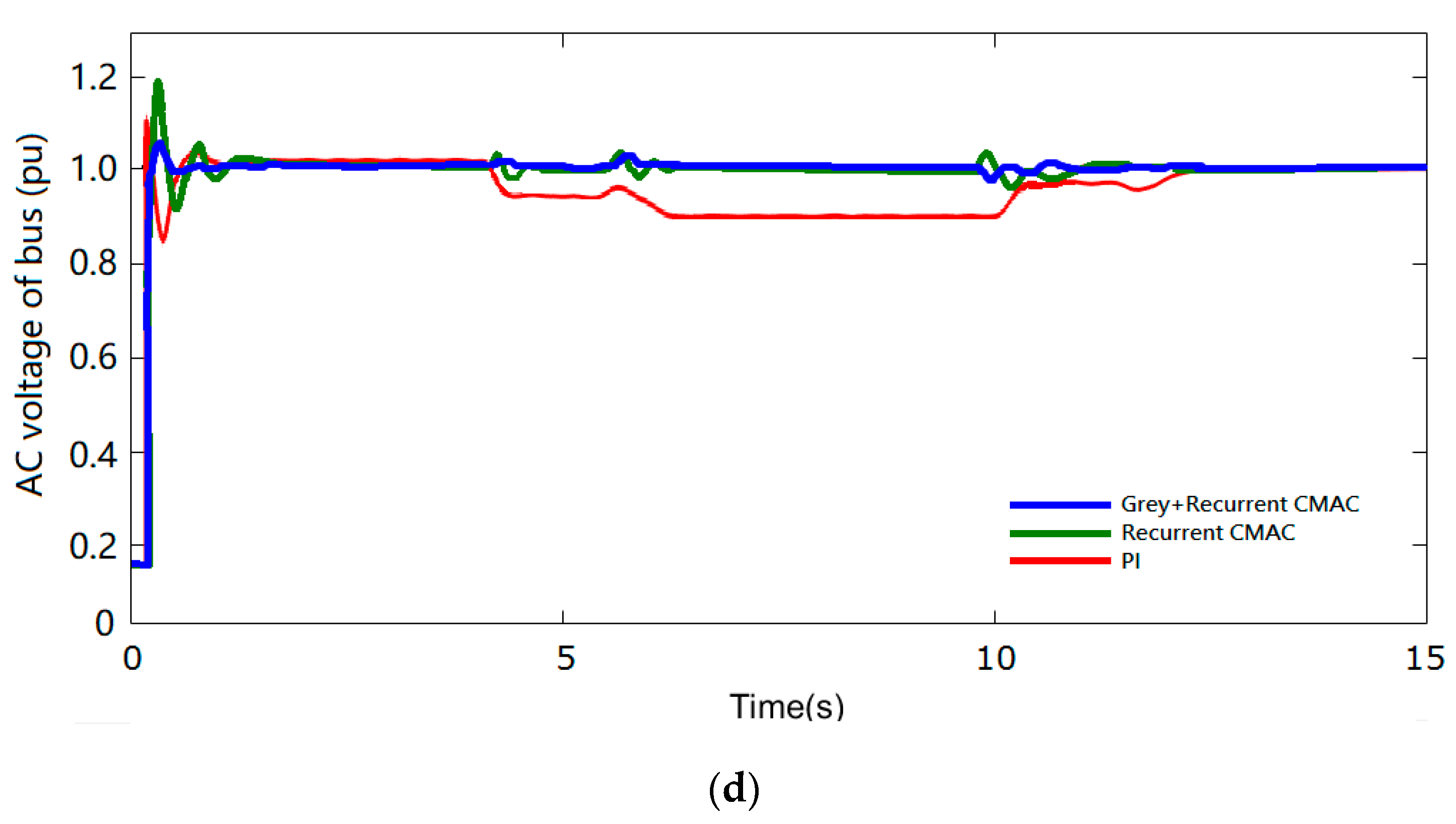
4.4. Short-Circuit Fault of Power Grid

This case simulates a short-circuit fault that occurs suddenly for a period of 0.1 s when the grid is at 2 s. Figure 7 shows the transient response of the studied system. This simulation aims to study the ability of WECS to resume stable operation after short-circuit fault. Figure 7a shows that the PMSG’s rotor speed can more quickly return to the steady state with the proposed method than with other methods. Figure 7b,c shows the dynamic responses of real and reactive power for WECS, respectively. When the Grey–RCMAC with IPSO is used, the power shows smaller oscillations than the RCMAC. Figure 7d shows the transient performance of the AC bus voltage at the PMSG grid side when a fault occurs. The AC bus voltage shows deeper sag with the proposed method than with the other three methods. The recovery time of the voltage response of the PI controller is the longest (i.e., approximately 2.5 s), although it is still observed that the voltage response has a slight oscillation. Table 4 lists the numerical comparison results of the PI, RFNN, CMAC, RCMAC, and Grey–RCMAC with IPSO controller when a fault occurs.

5. Conclusions

The hybrid Grey–RCMAC and IPSO method proposed is applied to a wave power system herein. The effectiveness of power operation control and grid stability of the method is verified by case analysis. Results show that the proposed control scheme exhibits strong robustness and effectiveness to both dynamic and transient capabilities in the event of system load changes and sudden short-circuit faults in the grid. The control performance shows that the proposed control scheme can effectively stabilize the operation of the power grid under unstable conditions, reduce power oscillation, and quickly return to steady state. In comparison with the earlier methods, the hybrid Grey–RCMAC has better response time and convergence error performance and can be incorporated to ensure system robustness under different environmental effects. Thus, the Grey GM(1,1) model has higher accuracy and better fitting effect for exponential type signal prediction. The method takes advantage of simplicity and less required computation time, and the proposed controller realizes the feedback that guarantees system stability and disturbance resistance.

Experimental evaluations on real data are future work in this paper. The proposed hybrid Grey–RCMAC topology has been tested by using the experimental system. The control algorithm for the emulation of the Wells-turbine-driven PMSG is implemented in the DSP board. All the control schemes are implemented by using a real-time workshop (RTW), which is online trained by PSCAD/EMTDC and implemented by dSPACE. The real-time process is running in a dSPACE that includes a TMS320C67x floating-point DSP.

References

1. Halamay, D.; Brekken, T.; Simmons, A.; McArthur, S. Reserve requirement impacts of large-scale integration of wind, solar and ocean wave power generation. IEEE Trans. Sustain. Energy 2011, 2, 321–328. [Google Scholar] [CrossRef]
2. Zhao, X.; Yan, Z.; Zhang, X.P. A wind-wave farm system with self-energy storage and smoothed power output. IEEE Access 2016, 4, 8634–8642. [Google Scholar] [CrossRef]
3. Linda, S.; Rachel, S.; Thomas, D. What drives energy consumers: Engaging people in a sustainable energy transition. IEEE Power Energy Mag. 2018, 16, 20–28. [Google Scholar]
4. Nicola, D.; Davide, B.; Francesco, G.; Paolo, C.; Giampaolo, B. Review of oscillating water column converters. IEEE Trans. Ind. Appl. 2016, 52, 1698–1710. [Google Scholar]
5. Romain, G.; Josh, D.; John, V.R. Adaptive control of a wave energy converter. IEEE Trans. Sustain. Energy 2018, 9, 1588–1595. [Google Scholar]
6. Murthy, B.K.; Rao, S.S. Rotor side control of Wells turbine driven variable speed constant frequency induction generator. J. Electr. Power Compon. 2005, 33, 587–596. [Google Scholar] [CrossRef]
7. Oscar, B.; José, A.C.; José, M.G.d.D.; Patxi, A. A real time sliding mode control for a wave energy converter based on a Wells turbine. Ocean Eng. 2018, 163, 275–287. [Google Scholar]
8. Oscar, B.; Isidro, C.; José, M.G.d.D. Adaptive sliding mode control for a control for a double fed induction generator used in an oscillating water column system. Energies 2018, 11, 1–27. [Google Scholar]
9. Albus, J.S. A new approach to manipulator control: The cerebellar model articulation controller (CMAC). J. Dyn. Syst. Control. 1975, 97, 220–227. [Google Scholar] [CrossRef] [Green Version]
10. Shiraishi, H.; Ipri, S.L.; Cho, D.D. CMAC neural network controller for fuel-injection systems. IEEE Trans. Control Syst. Technol. 1995, 3, 32–38. [Google Scholar] [CrossRef]
11. Kim, Y.H.; Lewis, F.L. Optimal design of CMAC neural network controller for robot manipulators. IEEE Trans. Syst. Man Cybern. C Appl. Rev. 2000, 30, 22–31. [Google Scholar] [CrossRef]
12. Chiang, C.T.; Lin, C.S. CMAC with general basis functions. J. Neural Netw. 1996, 9, 1199–1211. [Google Scholar] [CrossRef]
13. Wang, S.Y.; Tseng, C.L.; Yeh, C.C. Adaptive supervisory Gaussian-cerebellar model articulation controllers for direct torque control induction motor drive. IET Electr. Power Appl. 2011, 5, 295–306. [Google Scholar] [CrossRef]
14. Yeh, M.F.; Tsai, C.H. Standalone CMAC control systems with online learning ability. IEEE Trans. Syst. Man Cybern. B 2010, 40, 43–53. [Google Scholar]
15. Bhattacharya, R.; Bhattacharya, T.K.; Garg, R. Position mutated hierarchical particle swarm optimization and its application in synthesis of unequally spaced antenna arrays. IEEE Trans. Antennas Propag. 2012, 60, 3174–3181. [Google Scholar] [CrossRef]
16. Srivastava, L.; Dixit, S.; Agnihotri, G. Optimal location and sizing of TCSC for voltage stability enhancement using PSO-TVAC. In Proceedings of the 2014 Power and Energy Systems: Towards Sustainable Energy, Bangalore, India, 13–15 March 2014; pp. 1–6. [Google Scholar]
17. Lin, W.M.; Lu, K.H.; Huang, C.H.; Ou, T.C.; Li, Y.H. Optimal location and capacity of STATCOM for voltage stability enhancement using ACO plus GA. In Proceedings of the 2009 IEEE/ASME International Conference on Advanced Intelligent Mechatronics, Singapore, 14–17 July 2009; pp. 1915–1920. [Google Scholar]
18. Wang, L.; Chen, Z.J. Stability analysis of a wave-energy conversion system containing a grid-connected induction generator driven by a Wells turbine. IEEE Trans. Energy Convers. 2010, 25, 555–563. [Google Scholar] [CrossRef]
19. Tomonobu, S.; Yasutaka, O.; Yasuaki, K.; Motoki, T.; Atsushi, Y.; Endusa, B.M.; Naomitsu, U.; Toshihisa, F. Sensorless maximum power point tracking control for wind generation system with squirrel cage induction generator. Renew. Energy 2009, 34, 994–999. [Google Scholar]
20. Lin, W.M.; Hong, C.M.; Cheng, F.S. Design of intelligent controllers for wind generation system with sensorless maximum wind energy control. Energy Convers. Manag. 2011, 52, 1086–1096. [Google Scholar] [CrossRef]
21. Krause, P.C. Analysis of Electric Machinery; McGraw-Hill: New York, NY, USA, 1986. [Google Scholar]
22. Erenturk, K. Hybrid control of a mechatronic system: Fuzzy logic and grey system modeling approach. IEEE Trans. Mechatron. 2007, 12, 703–710. [Google Scholar] [CrossRef]
23. Deng, J.L. Introduction to grey system theory. J. Grey Syst. 1989, 1, 1–24. [Google Scholar]
24. Lin, W.M.; Hong, C.M.; Huang, C.H.; Ou, T.C. Hybrid control of a wind induction generator based on Grey–Elman neural network. IEEE Trans. Control Syst. Technol. 2013, 21, 2367–2373. [Google Scholar] [CrossRef]
25. Lin, C.M.; Chen, C.H. Car-following control using RCMAC. IEEE Trans. Veh. Technol. 2007, 56, 3660–3673. [Google Scholar] [CrossRef]
26. Lin, C.M.; Hsu, C.F. Neural network hybrid control for antilock braking systems. IEEE Trans. Neural Netw. 2003, 14, 351–359. [Google Scholar] [CrossRef] [PubMed]
27. Lin, C.M.; Hsu, C.F. Supervisory recurrent fuzzy neural network control of wing rock for slender delta wings. IEEE Trans. Fuzzy Syst. 2004, 12, 732–742. [Google Scholar] [CrossRef]
28. Jacob, R.; Yahya, R.S. Particle swarm optimization in electromagnetics. IEEE Trans. Antennas Propag. 2004, 52, 397–407. [Google Scholar]
29. Varshney, S.; Srivastava, L.; Pandit, M. Optimal location and sizing of STATCOM for voltage security enhancement using PSO-TVAC. In Proceedings of the 2011 International Conference on Power and Energy Systems, Chennai, India, 22–24 December 2011; pp. 22–24. [Google Scholar]
30. Oh, Y.J.; Park, J.S.; Hyon, B.J.; Lee, J. Novel control strategy of wave energy converter using linear permanent magnet synchronous generator. IEEE Trans. Appl. Supercond. 2018, 28, 1–5. [Google Scholar] [CrossRef]
31. Prudell, J.; Stoddard, M.; Amon, E.; Brekken, T.K.A.; von Jouanne, A. A permanent magnet tubular linear generator for ocean wave energy conversion. IEEE Trans. Ind. Appl. 2010, 46, 2392–2400. [Google Scholar] [CrossRef]
32. Lin, W.M.; Hong, C.M. A new Elman neural network-based control algorithm for adjustable-pitch variable speed wind energy conversion systems. IEEE Trans. Power Electron. 2011, 26, 473–481. [Google Scholar] [CrossRef]
Figure 1. Schematic diagram of a PMSG-based Wells turbine system.
Energies 13 00241 g001
Figure 2. Proposed RCMAC architecture.
Energies 13 00241 g002
Figure 3. Output power tracking response of the WECS.
Energies 13 00241 g003
Figure 4. Dynamic responses to speed changes for the studied system: (a) Wells turbine’s rotor speed response, (b) the real power response of WECS, (c) the reactive power response of WECS, and (d) dynamic voltage amplitude response of AC bus on power grid side.
Energies 13 00241 g004aEnergies 13 00241 g004b
Figure 5. Dynamic responses to pressure drop for the studied system: (a) the pressure variation, (b) the real power response of WECS (Case 1), (c) Wells turbine’s rotor speed response (Case 1), (d) the real power response of WECS (Case 2), and (e) Wells turbine’s rotor speed response (Case 2).
Energies 13 00241 g005aEnergies 13 00241 g005bEnergies 13 00241 g005c
Figure 6. Dynamic responses of the studied system with load changes: (a) Wells turbine’s rotor speed response, (b) the real power response of WECS, (c) the reactive power response of WECS, and (d) dynamic voltage amplitude response of AC bus on power grid side.
Energies 13 00241 g006aEnergies 13 00241 g006b
Figure 7. Transient responses of the studied system when a fault occurs: (a) generator speed of WECS (b) real power of WECS, (c) reactive power of WECS, and (d) transient voltage amplitude response of AC bus on power grid side.
Energies 13 00241 g007aEnergies 13 00241 g007b