A Decision Support System Tool to Manage the Flexibility in Renewable Energy-Based Power Systems

Abstract

Renewable Energy Sources (RES) have taken on an increasingly important role in the energy mix in the last few years, and it has been forecasted that this trend will continue in the future. The energy production from these sources is not dispatchable, and the increasing penetration of RES in energy mixes may therefore lead to a progressive loss of generation control and predictability. It has become clear that, to reach higher RES penetration levels, it is essential to increase power system flexibility in order to ensure stable operations are maintained. An ICT (Information and Communication Technology) tool that may be used to manage and optimize the flexibility offered by energy storage and conversion systems is described in this paper with specific reference to the Decision Support System (DSS) developed within the H2020 PLANET (PLAnning and operational tools for optimizing energy flows and synergies between energy NETworks) project. The paper focuses on how the PLANET DSS tool evaluates, manages, and dispatches the flexibility of Power to Gas/Heat (P2X) technologies. Moreover, the tool has been used to analyze a realistic case in order to show how the PLANET DSS tool could be used to evaluate the energy and economic benefits of taking advantage of the flexibility of P2X technologies.

1. Introduction

The world’s mean temperature has risen by 0.8 °C since the beginning of the twentieth century [1] due to an increase in anthropogenic greenhouse gas emissions [2]. The European Union (EU) has outlined ambitious objectives to reduce this dangerous trend [3,4]. Renewable Energy Sources (RES) will play a fundamental role in the near future, as the power sector alone is responsible for around 30% of global emissions [5]. Because of the intrinsic nature of RES, the energy production of these sources is not dispatchable, and as their share of the energy mix increases, so will the challenges concerning the balancing of consumption and generation.

In an increased RES penetration scenario, a greater degree of flexibility in the energy dispatch system is required to handle unpredictable variations of energy production and facilitate the RES integration in the existing infrastructures [6]. The key requirements to achieve proper grid operations include a wide range of technologies and solutions, such as energy storage (e.g., Virtual Energy Storage VES [7,8]), energy conversion (e.g., Power-to-Gas (P2G) [9,10] and Power-to-Heat (P2H) [11]), which allow flexibility to be increased thanks to interconnections between energy sectors [12,13]. Moreover, energy systems are becoming more and more costumer centric, and in this context it becomes very important to be able to define appropriate systems of measurement and prediction of energy flows [14] in order to be able to analyze the flexibility potential within energy systems.

In these scenarios, energy flows within energy systems are somewhat complicated and intricate, due to the interconnection of different energy networks and the increase in stochasticity resulting from distributed generation. For this reason, it is important to have computer simulation tools available to analyze these interconnected energy flows and to evaluate the energy and economic impact of different technologies and regulations on the entire system [15,16].

A specific ICT DSS tool has been proposed by The EU-Funded H2020 PLANET project [17] to analyze and optimize the flexibility of P2X energy conversion technologies. The project provides an ICT platform to support network operators/planners, P2X plant managers, load aggregators, and policy makers in order to increase the integration of renewables.

Several software programs are available in the literature to simulate energy flows in a Multi Energy System (MES) [16,18,19]. The main advantage of using the PLANET DSS lies in the fact that the tool is built on a web platform: through the web platform, the users can setup and execute a remote simulation, and in this way the various actors can benefit from using a dedicated super-computer for their simulation, to which they would otherwise not have access. Moreover, due to middleware-based communication, Demand-Response (DR) signals exchanged between the tool modules (e.g., the output of the flexibility usage optimization module) can easily be transmitted to real-world equipment in order to update DR commands. In this way, the functionality of the PLANET platform is superior to that of a typical simulation tool, as it may be used by DSOs to perform DR scheduling, if appropriate Machine-to-Machine (M2M) interfaces are developed. An important feature of the tool is that the different mathematical models and modules interact with a seamless exchange of data in a co-simulation process. The co-simulation of the different modules (see also reference [20]) makes DSS very flexible and scalable, and as such each module can easily be modified or replaced in a plug and play fashion. The PLANET platform allows existing P2X unit managers to register their unit model and perform simulations in order to assess whether it would be beneficial for their units to participate in DR operations.

This paper is a progression of the work presented in references [21,22]. In the previous work, the role of each component involved in the PLANET architecture was explained, while this paper focuses on the particular aspect of how the flexibility of the energy conversion technologies is evaluated and managed within PLANET DSS. In order to better clarify the strengths of the PLANET tool, a description of a use case, where the flexibility of a P2G plant is used to alleviate Reverse Power Flow (RPF) issues caused by excess RES generation, has been included in the paper. The case study is used as an example to show how the tool optimizes P2X utilization as a function of the available flexibility and the energy flows in the grid. A schematic representation of the analyzed energy system is shown in Figure 1, together with the involved energy flows and the energy conversion plants that act as connectors between the networks.

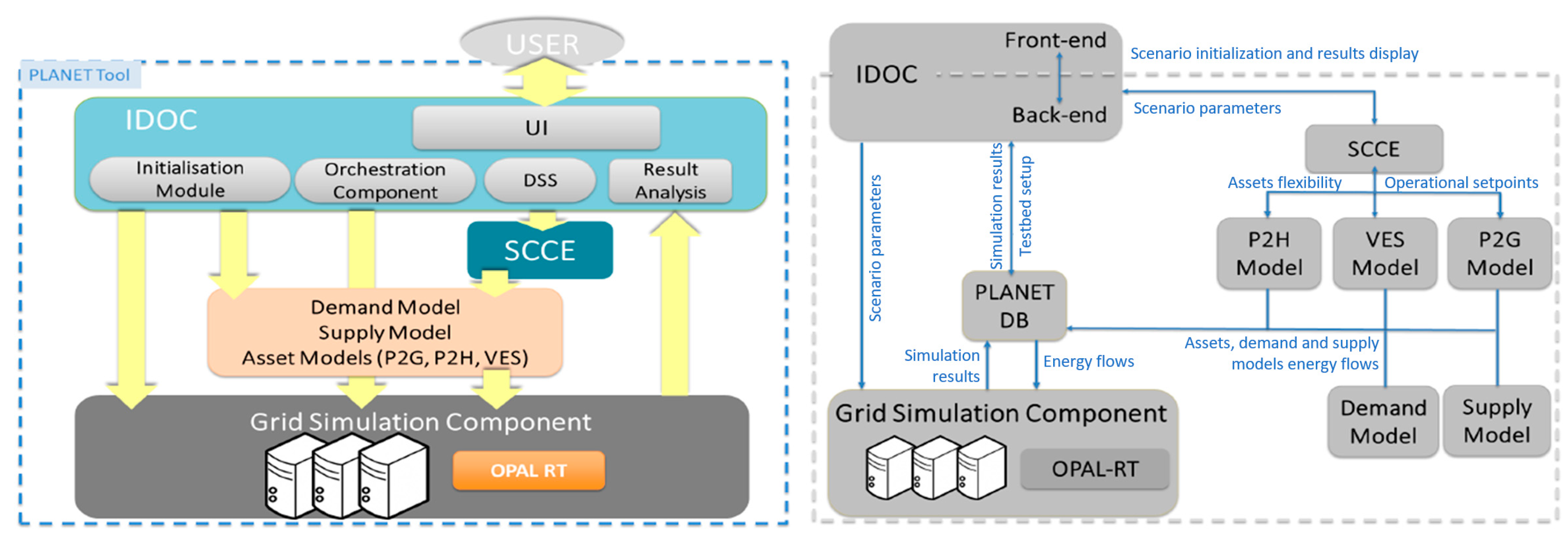
2. The PLANET Solution: System Architecture

The main functional components of the PLANET DSS are:

• The user interface and orchestration module: the Integrated Decision Support System and Orchestration Cockpit (IDOC) component;
• Energy Demand, Supply, and Asset (P2G, P2H, VES) modules;
• The optimization module: District-level Storage/Conversion Coordination Engine (SCCE) module;
• The Grid Simulation component.

Figure 2 reports the high-level architecture of the PLANET tool, identifies all the different ICT components, and shows how they are related to each other.

As indicated in Figure 2, the user can interact with the PLANET tool through the IDOC front-end, which is accessible via a web-based User Interface (UI). Through the UI, the user can initialize the energy scenario (by defining the networks, demand/supply modules, and grid-connected asset parameters) and, at the end of the simulation, can visualize the results. The energy scenario is saved in the PLANET Database (DB) and all the initialization parameters are then dispatched, by the IDOC back-end, to the corresponding modules.

The asset models are developed in the MATLAB/Simulink environment. Each flexible asset receives from the SCCE controller the optimum working set-points, the energy consumption/generations of these modules is saved in the DB and sent to the grid simulation component. The mathematical models of the assets are validated by real data from the pilot plants of the project: one in France for VES and one in Italy for P2H [21]. Meanwhile, the P2G model are validated using data obtained from the high-fidelity P2G process simulator model, which is based on the Apros^® simulator [23] developed in the Neo Carbon Energy project [24].

Depending on the operating parameters defined by the user and the working conditions at each time step of the simulation, each asset can offer a certain degree of flexibility to the system (This concept is defined in more detail in Section 3). The SCCE, developed as a Phyton script, calculates the optimal operation set-points of the assets (P2G, P2H, VES) according to the available flexibility and the grid requirements. The optimization algorithm has been set in order to optimize the network energy flows, and in particular to reduce the Reverse Power Flow. For more information about the optimization process performed by SCCE, please see reference [25]. The grid simulator component receives the energy flows of all the involved modules, performs a power flow calculation (the power flow will be solved with the eMEGAsim Power Grid simulator of OPAL-RT [26]), provides the simulation results to the PLANET DB and to the IDOC back-end for the visualization of the simulation results. The OPAL-RT simulator allows the behavior of the power grids to be simulated in detail. This software has already been widely used in literature for the analysis of electrical networks [27,28,29].

2.1. The PLANET DSS ICT Tool

PLANET DSS comprises several frontends (User Interfaces) and backend components. The main functionalities are (i) the setting up a simulation scenario, (ii) transferring the scenario and executing the simulation at the central simulator, (iii) visualizing the results. Moreover, additional functionalities are available, such as a comparison of the results of previously run simulations.

The backend components are grouped into two main categories, which are outlined below.

2.1.1. PLANET Middleware

The middleware is a cloud platform that typically allows devices such as meters and sensors to be registered in order to collect measurements from these “field” devices and forward them to ICT modules that utilize this information for higher-level functionalities. In addition, in the case of field actuators, the middleware can route operating commands from the cloud to the actuators. The middleware usage in PLANET can be two-fold:

• it is currently used to set up simulators as devices, in such a way that the operator is able to select between different simulator providers. After its configuration, the middleware routes the simulation control commands from the PLANET IDOC (web-app UI) to the preconfigured simulator;
• in the next PLANET prototype, it will be used to route the communications between the central simulator that calculates the power flow of the grid section under investigation and the remote simulators that model the operation of the P2X and VES units, that is, it will a) transmit flexibility information from the unit models to the central simulator and b) receive unit operating points from the SCCE. Once this has been achieved, the “co-simulation” scenarios that implement an envisioned real-world system operation will be tested and evaluated.

2.1.2. Backend Orchestration Scripts

These scripts are responsible for the synchronization and serialization of operations of the various components of the system. Indicatively, the following scripts can be mentioned:

• scripts that can be used to retrieve topology information about the grid and the energy resources connected to the grid nodes. This information is created by the user, via the IDOC UI, and the scripts translate these parameters into properly structured files (JavaScript Object Notation JSON) that are then used by the simulator;
• scripts that can be used to retrieve uncontrollable electricity and heat demands and formulate them according to the simulation time-step and horizon that the user selects via the UI. These files are currently stored statically in the backend of the platform. This information is supposed to be provided by the Distribution System Operators of electric and heat networks (DSO-e, DSO-h). For the grid-planning use of the PLANET system, this information comes from historical measurements covering a timespan of one year. It has been envisioned that for the operational use, these files will be dynamically created, as outputs of the load (heat and electricity) forecasting algorithms that the DSOs employ;
• scripts that can be used to retrieve meteorological, photovoltaic (PV), and Wind turbine generation data utilizing the renewable.ninja service [30] according to the location chosen by the user. The scripts retrieve the physical and operating characteristics of the PV and wind turbines that may be connected to the electric branch nodes and create the request according to the appropriate structure dictated by the renewables.ninja Application Program Interface (API). The results are then stored in the PLANET DB for use by the simulator. The RES parameters and their connection nodes are specified by the user, via the IDOC UI, as part of the simulation scenario creation process;
• scripts that can be used to retrieve simulation results and (a) present them to the user via visualizations and charts and (b) store them in the PLANET MongoDB database. Other scripts that fall into the same category are the ones that handle the comparison of results from two or more previously executed simulations.

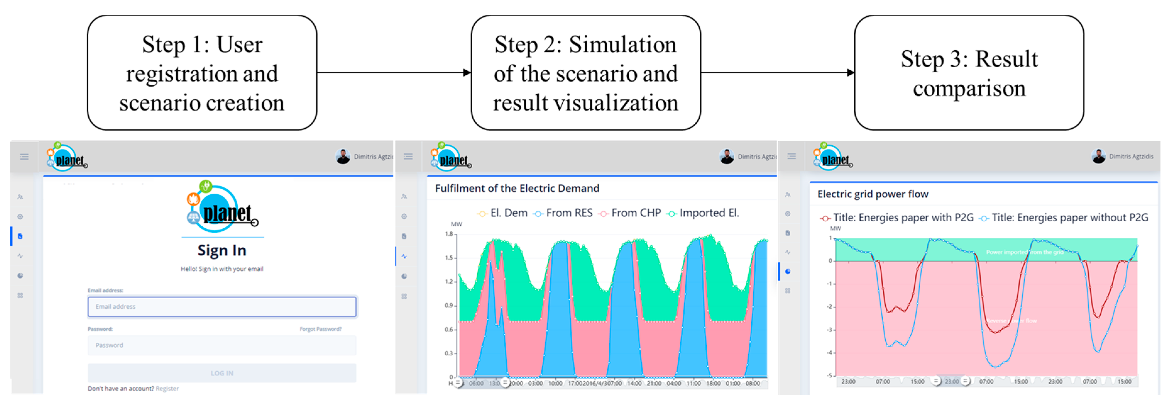
2.1.3. Frontend Web User Interface

The frontend is the web-based interface that the user accesses in order to set up and execute a simulation. Several functionalities have been included in this preliminary operational prototype:

• scenario creator: in this UI section, the user is able to create a simulation scenario in a step-by-step manner so as to avoid overloading the user. The scenario includes the name, description, the selection of the electric grid template from those already stored in the system (provided by the DSOs), the adding, editing, and deleting of renewables, loads, and flexibility units at each grid node, the editing of the properties of each of the aforementioned technologies, and the adding of economic parameters regarding the CAPEX and OPEX of the units, as well as emissions-related costs;
• simulation execution: in this section, the user is able to select a previously created scenario and instruct the remote simulator to execute it. This is done via the previously mentioned backend scripts. After the simulation has been performed, the results are visualized for the user. The results include energy flows between the energy networks, the power timeseries values and energy values over the entire simulation horizon, economic results (e.g., Levelized Cost of Electricity (LCOE)), carbon dioxide (CO2) emissions, and the Simple Payback period (SP) of the technologies;
• simulation comparison: in this section, the user is able to select two or more previously run simulations and compare the results.

The flowchart of the PLANET DSS UI utilization steps is depicted in Figure 3. In the first step, the user registers himself/herself and creates a new energy scenario (location, horizon, grids, technologies and economic parameters). In the second step, the user starts the scenario simulation and visualizes the results (for example, the fulfillment of the electricity demand through different energy sources, as reported in Figure 3). In the third step, the user can compare the obtained results with a previous scenario (for example, Figure 3 compares the electric power withdrawn from the external electricity network for two different scenarios).

3. Flexibility in the PLANET Architecture

Flexibility may be defined as the capability of a system to modify its energy generation/consumption profile in order to offer ancillary services to the grid. It is possible to define negative and positive forms of flexibility [31]. The following convention has been used in this paper: positive flexibility is defined as the capability of a system to increase its energy consumption or, equivalently, to reduce its production. Positive flexibility may be required when the RES generation exceeds the total load and there is a need to balance the energy in the network in order to maintain grid stability, for example by converting or storing excess RES energy. Negative flexibility is the capacity of a system to decrease the total energy consumption in the system itself, or to increase the total energy production [32], and this may be required when the RES production is lower than the total load or during a critical peak pricing event.

In an energy system scenario, flexibility can be provided by different technologies, for example:

• pure load units (e.g., Electric vehicle charging stations [33]) can provide positive and negative flexibility by increasing/decreasing their electric load;
• energy storage systems can offer positive flexibility by absorbing energy from the grid or negative flexibility by releasing stored energy [34];
• energy conversion units (P2G, P2H) can offer both positive and negative flexibility by modifying their operation set-points [35];
• generation units (e.g., Combined Heat and Power CHP) can increase/decrease the power introduced into the network and they therefore offer flexibility [36];
• the RES sources could also provide flexibility by modulating the power production (with the constraint of the variable maxim output being driven by the weather conditions) [37,38].

The Power Node approach, proposed in reference [39], had been adopted to calculate and evaluate the available flexibility. The advantage of this method is that it can be used to define the flexibility of any conceivable power system with the same mathematical equations. For the sake of clarity, the same nomenclature proposed in reference [39] has been maintained, while the sign convention has been modified slightly in order to better clarify the power flow in the present cases. Figure 4 reports all the possible power exchanges between the electric grid and a general device. The same notations could be adopted for power generation plants, power conversion units (P2G, P2H), electric storages, and for pure load units.

where:

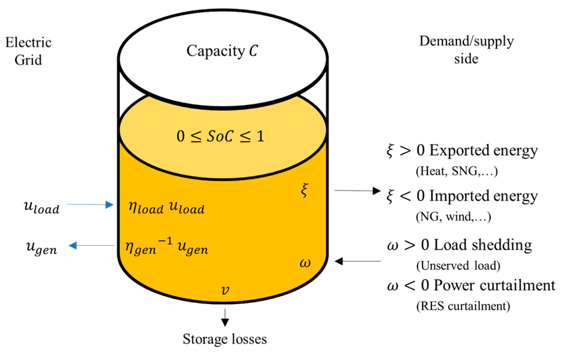
• $C\ge 0$ [MWh] is the internal storage capacity ($C=0$, for a non-buffered unit);
• $0\le SoC\le 1$ is the normalized State of Charge;
• $u_{load}\ge 0$ [MW] is the electric consumption of the device and ${\eta }_{load}$ is the charging/conversion efficiency;
• $u_{gen}\ge 0$ [MW] is the electric generation of the device and ${\eta }_{gen}$ is its efficiency;
• $\xi$ [MW] is the energy flow that exits the system ($\xi >0$ e.g., Synthetic Natural Gas SNG, heat) or the energy flow that enters into the system ($\xi <0$, e.g., Natural Gas NG, wind energy) by the device;
• $\omega$ [MW] represents an unserved load ($\omega >0$, e.g., demand curtailment) or an enforced energy loss ($\omega <0$, e.g., RES curtailment);
• $v\ge 0$ [MW] is the energy storage loss.

The general Power Node equation is:

$$C \dot{SoC}={\eta }_{load} u_{load}-{\eta }_{gen}{}^{-1} u_{gen}-\xi +\omega -v.$$

(1)

Generally, each term in the above equation may be either controllable or non-controllable. $v$, η_load and ${\eta }_{gen}$. may be fixed or state dependent (e.g., $v=f\left(SoC\right)$).

The electricity load/generator of the device is constrained as:

$$0\le u_{load}^{min}\le u_{load}\le u_{load}^{max}$$

(2)

$$0\le u_{gen}^{min}\le u_{gen}\le u_{gen}^{max}$$

(3)

$${\dot{u}}_{load}^{min}\le {\dot{u}}_{load}\le {\dot{u}}_{load}^{max}$$

(4)

$${\dot{u}}_{gen}^{min}\le {\dot{u}}_{gen}\le {\dot{u}}_{gen}^{max}.$$

(5)

Equations (2) and (3) represent the maximum and minimum power generation/load, which are normally defined on the basis of the nominal power and the minimum working power. Equations (4) and (5) pertain to the restriction due to the ramp rate capacity of the device. More details on Power Node modeling are reported in references [39,40,41].

If a general P2X energy conversion device is considered as an example, the Power Node equation for the $k$ simulation time step, can be written as:

$$u_{P2X}\left(k\right) = \frac{\left( {\xi }_{P2X}\left(k\right)+C{\dot{ SoC}}_{P2X}\left(k\right)+v_{P2X}\left(k\right)\right)}{{\eta }_{P2X}}$$

(6)

where term $C$ is the internal energy storage capacity (e.g., a heat storage of a P2H or a SNG vessel for P2G), $So{C}_{P2X}$ is its normalized State of Charge and $v_{P2X}$ is its energy loss. ${\xi }_{P2X}$ is the X energy vector provided externally and ${\eta }_{P2X}$ is the efficiency of the P2X process. The unit can modify its electric load, $u_{load,P2X}$, by modifying the internal storage SoC and/or the X energy exported outside the plant.

For a load unit, the available flexibility can be defined as:

$${\pi }_{P2X}\left(k\right)=u_{P2X}^{feasible}\left(k\right)-u_{P2X}^0\left(k\right)=\frac{\left({\xi }_{P2X}^{feasible}\left(k\right)+C{\dot{SoC}}_{P2X}^{feasible}\left(k\right)+v_{P2X}\left(k\right)\right)}{{\eta }_{P2X}}-u_{P2X}^0\left(k\right)$$

(7)

where $u_{P2X}^{feasible}$ is the electric load of the unit in one of the possible working conditions and $u_{P2X}^0$ is the unit electricity load. The ${\xi }_{P2X}^{feasible}$ term is the amount of X energy that may be exported outside the plant without violating the external constraints (e.g., the district heating or gas grid capacity). It is possible to define ${\xi }_{P2X}^{max}\ge 0$ and ${\xi }_{P2X}^{min}\ge 0$; these represent the maximum and minimum flows of energy vector X that may be exported. Term $C{\dot{SoC}}_{P2G}^{feasible}$ may be positive or negative, and is bound by a maximum $C{\dot{SoC}}_{P2X}^{max}\ge 0$ and a minimum $C{\dot{SoC}}_{P2X}^{min}\le 0$, depending on the buffer condition (e.g., when the buffer reaches full charge, $C{\dot{SoC}}_{P2X}^{max}=0$).

The electric load of the unit is bound by the constraints:

$$0\le u_{P2X}^{min}\le u_{P2X}^{feasible}\left(k\right)\le u_{P2X}^{max})$$

(8)

$${\dot{u}}_{P2X}^{min}\le {\dot{u}}_{P2X}^{feasible}\left(k\right)\le {\dot{u}}_{P2X}^{max}).$$

(9)

Combining Equations (7)–(9), it is possible to define the positive and negative power capacity flexibility (${\pi }^{+},{\pi }^{-}$):

$${\pi }_{P2X}^{+}\left(k\right)=min\left\{\frac{\left({\xi }_{P2X}^{max}\left(k\right)+C{\dot{SoC}}_{P2X}^{max}\left(k\right)+v_{P2X}\left(k\right)\right)}{{\eta }_{P2X}},u_{P2X}^{max},u_{P2X}^0\left(k\right)+{\dot{u}}_{P2X}^{max}\Delta k\right\}-u_{P2X}^0\left(k\right)$$

(10)

$${\pi }_{P2X}^{-}\left(k\right)=max\left\{\frac{\left({\xi }_{P2X}^{min}\left(k\right)+C{\dot{SoC}}_{P2X}^{min}\left(k\right)+v_{P2X}\left(k\right)\right)}{{\eta }_{P2X}},u_{P2X}^{min} ,u_{P2X}^0\left(k\right)+{\dot{u}}_{P2X}^{min}\Delta k\right\}-u_{P2X}^0\left(k\right).$$

(11)

The terms $\frac{\left({\xi }_{P2X}^{min}\left(k\right)+C{\dot{SoC}}_{P2X}^{min}\left(k\right)+v_{P2X}\left(k\right)\right)}{{\eta }_{P2X}}$ and $\frac{\left({\xi }_{P2X}^{max}\left(k\right)+C{\dot{SoC}}_{P2X}^{max}\left(k\right)+v_{P2X}\left(k\right)\right)}{{\eta }_{P2X}}$ represent the storage and the external constraints at simulation step $k$. The limitation, due to the minimum and maximum power loads, is defined by $u_{P2X}^{min}$ and $u_{P2X}^{max}$. The terms $u_{P2X}^0\left(k\right)+{\dot{u}}_{P2X}^{min}\Delta k$ and $u_{P2X}^0\left(k\right)+{\dot{u}}_{P2X}^{max}\Delta k$ guarantee that the power increase/decrease during discretization interval $\Delta k$ does not exceed the ramp rate constraints.

The flexibility of the unit at step $k$ (${\pi }_{P2X}^{+}$ and ${\pi }_{P2X}^{-}$) is sent to and managed by the SCCE control system. Figure 5 reports the flexibility information flow. The flexibility generated by the energy storage/convention modules (VES P2G P2H) is sent to the SCCE. This component has the task of regulating the setpoints of the flexible components, according to their availability, and the generation and consumption of the network nodes. In short, the SCCE, when necessary, raises or lowers the setpoint of the flexible components in order to mitigate the problems of the networks. For more information on SCCE, see references [21,25].

4. Use Case Development

In order to demonstrate the current potential of PLANET’s preliminary operational prototype, the tool was used to simulate an energy scenario and then to improve its energy performance by exploiting the flexibility of a P2G system.

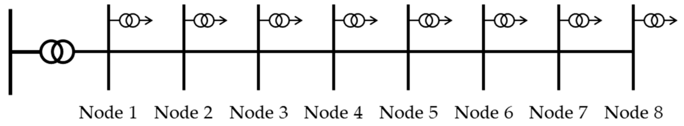
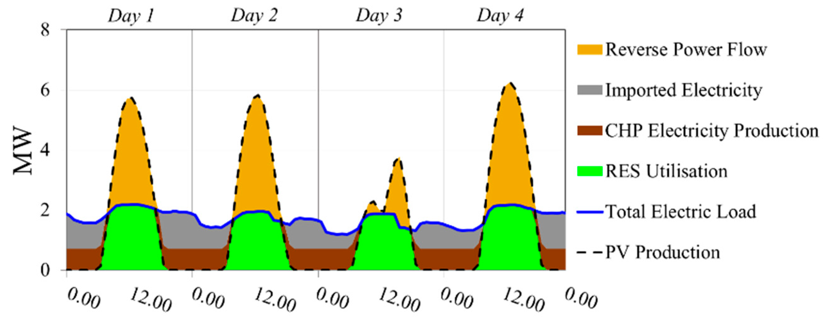
4.1. The Analyzed Scenario

The analyzed scenario represents a typical future scenario characterized by a high penetration of renewables that could cause problems for the electric grid. The possible energy flows are schematized in Figure 1. A medium voltage network feeder, consisting of eight nodes connected in series, was analyzed (see Figure 6). Uncontrollable loads, PV plants, a CHP plant, and a P2G asset are connected to the electric gird (see

Table 1. Technologies connected to the electric grid.

Grid Node	Electric Peak Load [MW]	PV Nominal Power [MW]	CHP -Nominal Power [MW]	P2G-Nominal Power [MW]
1	0.3	1.0	-	-
2	0.2	2.0	-	1.5
3	0.5	-	-	-
4	0.5	1.0	0.4	-
5	0.4	2.0	-	-
6	0.2	1.0	-	-
7	0.3	1.0	-	-
8	0.6	-	0.3	-
tot	3.0	8.0	0.7	1.5

).

Each node of the grid has been associated with an aggregated uncontrollable electric load. The uncontrollable load profile of the $i$-th node ($u_{node i}$) is defined as:

$$u_{node i}=p{u}_{el} P_{node i}$$

(12)

where $p{u}_{el}$ is the per-unit aggregated profile stored in the PLANET DB and $P_{nodei}$ is the aggregated peak load of the $i$ node defined by the user in the PLANET UI.

As for the uncontrollable load, the production from renewable sources was also determined using per-unit profiles ($p{u}_{PV}$), scaled according to the user defined installed power ($P_{nominal,PV}$). The per unit profiles are downloaded in the back-end of the UI from the renewable.ninja website [30], according to the user selected location of the RES plant (in this study, the scenario is located in the city of Turin, north-west Italy).

$$u_{PV }=p{u}_{PV} P_{nominal,PV}$$

(13)

The P2G system is composed of an electrolyzer and a methanizer. The electrolyzer converts electric power into hydrogen, which is then converted into SNG during the methanation process. The P2G process can be summarized by means of the following equation:

$$q_{SNG }={\eta }_{el} {\eta }_{meth} u_{P2G}={\eta }_{P2G} u_{P2G}$$

(14)

where $u_{P2G}$ is the electric input power, $q_{SNG}$ is the produced SNG energy flow, while ${\eta }_{el}$ and ${\eta }_{meth}$ are the conversion efficiencies of the electrolysis and methanation processes, respectively. All of the produced SNG is injected directly into the gas grid, whose capacity, for the sake of simplicity, has been assumed to be unlimited.

The CHP converts the chemical energy of the fuel (${\dot{m}}_{NG} LH{V}_{NG}$) into electricity ($u_{CHP}$) and heat ($q_{CHP}$):

$$u_{CHP }={\eta }_{ el chp} {\dot{m}}_{NG} LH{V}_{NG }$$

(15)

$$q_{CHP }={\eta }_{ el th} {\dot{m}}_{NG} LH{V}_{NG }.$$

(16)

It has been assumed that the District Heating (DH) supplies all the heat demand loads in the analyzed area. The heat is mainly produced by the CHP plants and from backup gas boilers (Gas to Heat G2H). The heat produced during the methanation process of the P2G plant supplies the DH network with a revenue of 45 €/MWh of heat.

The other parameters that need to be entered into the PLANET UI are summarized in

Table 2. Parameters required for scenario simulation.

Parameter	Value	Unit
Time horizon	1	years
Location	Turin	-
Time step	60	minutes
DH heat peak power	6.0	MW
G2H nominal power	6.0	MW
Electrolysis efficiency [42]	0.75	-
Methanation efficiency [42]	0.80	-
CHP electric efficiency [13]	0.40	-
CHP thermal efficiency [13]	0.45	-
P2G CAPEX 1 [43]	750–1550	€/kWe
P2G OPEX 2 [43]	4.0	% CAPEX
P2G Lifetime [43]	25	years

¹ Capital Expenditure (CAPEX). ² Operating Expenditure (OPEX).

.

The user may also change other parameters, whether of an economic or technology nature, but the default values proposed by the tool itself have been used for the present study.

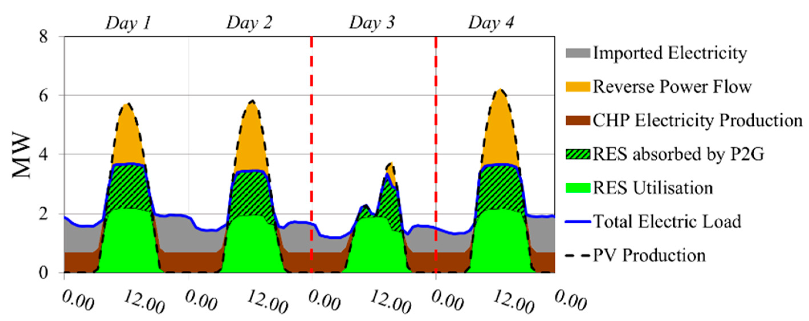
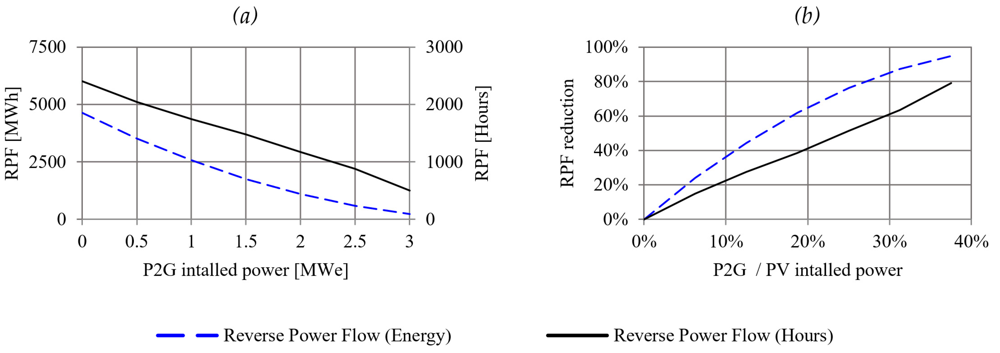
4.2. P2G Flexibility and the Objective Function

P2G systems can rapidly change their working set point, Polymer Electrolyte Membrane (PEM) electrolyzer can be completely ramped up and down (0÷100% range) in just a few seconds [10]. In order to make the hydrogen react with CO2 and produce SNG, the methanizer must be kept at the working temperature [44,45] and, for simplicity reasons, it was here considered that the methanizer is kept at the correct temperature during operation of the plant with no additional cost or energy consumption. The time step used in this analysis is one hour, and for this reason the P2G ramp constraint is negligible. The considered P2G system has no internal storage, and the produced SNG is considered to be injected directly into the NG network (whose capacity is considered unlimited). For this case study, the flexibility of P2G can therefore be rewritten as:

$${\pi }_{P2G}^{+}\left(k\right)= u_{P2G}^{max}-u_{P2G}^0\left(k\right)$$

(17)

$${\pi }_{P2G}^{-}\left(k\right)= u_{P2G}^{min}-u_{P2G}^0\left(k\right).$$

(18)

This flexibility can be used to optimize the operation of the system. In this study, operation of the P2G has been optimized, by the SCCE control, in order to absorb the overproduction of renewables and reduce the Reverse Power Flow. In fact, distributed generation energy scenarios, especially with a high RES penetration, may have to deal with an overproduction of energy as the uncontrolled production of renewables exceeds the instantaneous energy demand. When this happens, the over-production of energy is absorbed by the transmission network. This situation represents a non-optimal utilization of the renewables. Moreover, even though the Reverse Power Flow does not lead to a violation of the voltage and current limits, the protection scheme that is currently implemented in the distribution grid was not designed to handle the Reverse Power Flow, and for this reason the system is not able to guarantee adequate protection for the distribution system in such situations [46,47].

The SCCE receives the generation and consumption of the nodes and the flexibility of all the scenario assets (in this case only the P2G plant flexibility) as input. The objective of the control algorithm is to minimize the energy generation/consumption imbalance for each node of the network. In this way, the Reverse Power Flow is optimized indirectly. If it is not possible to balance generation and production in the unbalanced nodes (due to an insufficient flexibility present in that node), the SCCE exploits the flexibility of the assets installed in the nodes closest to the unbalanced one.

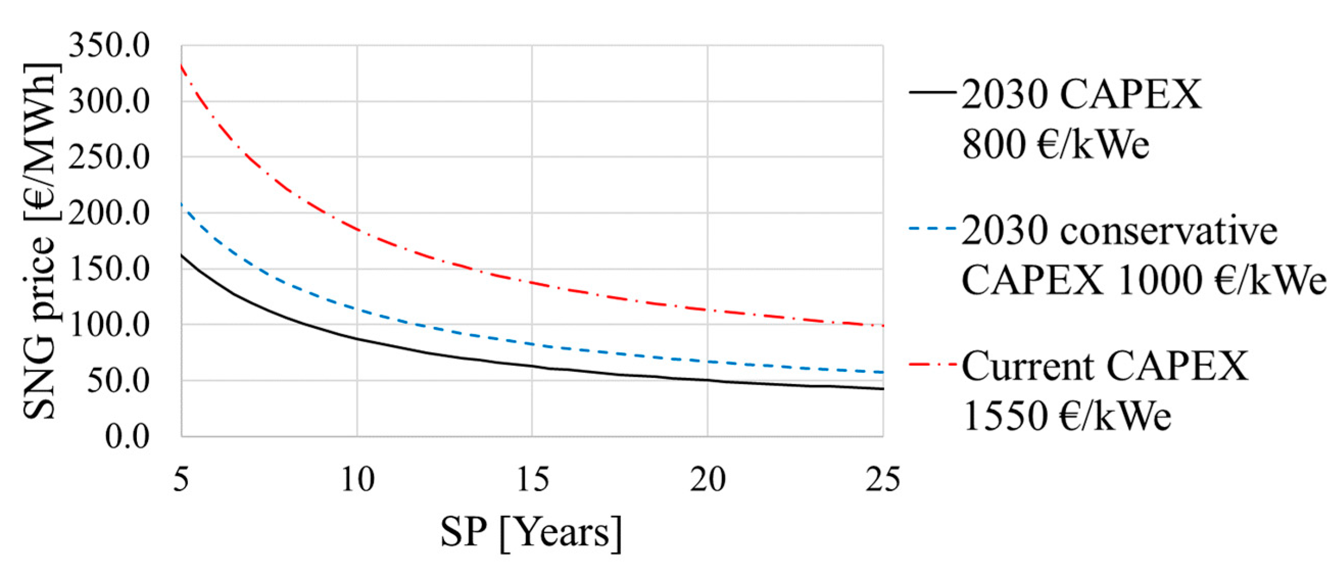
5. Results and Discussion

The PLANET tool was used to analyze the flexibility of a P2G plant and how its flexibility can be used in a high penetration renewable energy scenario. The scenario was first analyzed without any energy conversion assets and then with the installation of the P2G plant.

The aggregated electricity production and the electric load profiles in the analyzed gird branch for the case of no P2G installation are reported in Figure 7 for four typical days (in April). It can be seen that the load in the considered scenario is satisfied by the photovoltaic energy (53% on an annual basis), by the electricity produced by the CHP plants (21% on an annual basis) and by taking energy from the high voltage network (26% on an annual basis). Although the penetration of renewables in the considered scenario is around 50%, the large amount of installed PV power causes very high energy overproductions that are not consumed within the considered network. This overproduction amounts to about 40% of the total PV production and causes nearly 2400 hours of Reverse Power Flow during the whole year.

The energy flow of the same scenario, but with the installation of 1.5 MW of P2G, is depicted in Figure 8. It is possible to note that the flexible unit allows the electric load to be increased during RES overproduction, and this leads to an increase in the renewable energy utilization and a decrease in the Reverse Power Flow. The evolution of the flexibility of P2G is shown in Figure 9. At each time step, these flexibility values are sent to the SCCE controller (as schematized in Figure 5), which regulates the P2G Load (dashed gray curve) according to its flexibility and the grid power flows. The P2G system is not in operation at point 1, and the positive flexibility is therefore maximum since the plant could potentially increase its electric consumption up to the nominal power. The negative flexibility is zero, because the plant cannot further decrease its energy consumption. At this point, there is no overproduction of renewable energy (black dashed curve) and SCCE keeps the P2G turned off since there is no need to absorb any excess energy from the grid. The P2G is turned on at point 2 as the SCCE has detected an increase in renewable energy production. The positive P2G flexibility decreases as the plant is working closer to its nominal power, although, on the other hand, it gains negative flexibility as the plant is able to decrease the consumed power. In fact, control system exploits the generated negative flexibility at point 3 and uses it to lower the P2G set point in order to reduce the loads on the network.

P2G works at its nominal power at point 4. As such, the system controller cannot increase the surplus energy absorbed by P2G any further. At this point, the positive flexibility of P2G is zero as the plant is already working at is nominal capacity, and, at the same time, the negative flexibility reaches its maximum value. It can be noted that the P2G load follows and therefore completely absorbs the RES surplus up to point 3 thanks to the SCCE optimization control, while the P2G system is not able to absorb all the RES surplus energy between 15:00 and 16:00 due to its limited flexibility.

The PLANET tool was used to evaluate the scenario from an energy and an economic point of view. As reported in Figure 10a, even with 1.5 MW of P2G, the Reverse Power Flow, cannot be completely absorbed. Nevertheless, thanks to the flexibility of the 1.5 MW P2G plant, the Reverse Power Flow can be greatly reduced over the entire year: by more than 60 % in terms of energy and by about 40% in terms of duration. It is interesting to note that even with a small amount of installed P2G, compare to the PV nominal power, the effects on the Reverse Power Flow are remarkable. With an installed power of P2G equal to 10% of the PV nominal power, it is possible to achieve a reduction of the Reverse Power Flow of about 20% in terms of duration and about 40% in terms of energy (see Figure 10b).

Figure 11 compares the Simple Payback period (SP) with the price of the produced SNG, considering the current investment costs and the cost forecast for 2030, as proposed in reference [43]. The results obtained by the DSS show that, although the P2G plant benefits from the energy flows in the scenario, it may not be economically convenient due to the high investment costs and to the low full load hours of around 1900 per year. In fact, it can be noted that to have an SP of 10 years, considering the most optimistic CAPEX value, the SNG cost would need to be 85 €/MWh. Instead, considering the current CAPEX of these plants, the SNG would need to be incentivized to nearly 190 €/MWh in order to make this technology economically advantageous.

6. Conclusions

Because of the increase in distributed generation and the non-dispatchability of renewable energy sources, energy system simulation software has become fundamental to analyze the more and more complex energy systems that are emerging and to find the best solution from both an economic and an environmental point of view. The PLANET project has developed an ICT DSS tool for grid operators, P2X plant managers, and policy makers. This DSS tool was built specifically to analyze and optimize the flexibility of P2X energy conversion technologies. The tool can be used to analyze energy systems at a district scale. Through a web UI, it is possible to define the scenario that has to be analyzed by choosing the network loads, the technologies connected to the network, and their corresponding sizes. The user can also choose the geographical location of the scenario and, according to the user’s choice, the simulation is initialized with the corresponding meteorological and RES generation data.

The PLANET DDS tool has been introduced in this paper and how the flexibility of the involved technologies is managed within the tool has been analyzed in detail. Moreover, the mathematical model used to evaluate the available flexibility has been presented. The flexibility is calculated by means of the Power Node approach. This method is very powerful as it can be applied to any technology (whether generation or loads assets) that is connected to the electrical network.

An example of a possible case study has been presented in order to show how flexibility is managed and dispatched and, at the same time, to show the potential of the tool. The analyzed case study concerns a high penetration renewable energy scenario. When the scenario was first analyzed without any energy conversion assets, the tool allowed us to verify that even with a 50% renewable penetration, there are large energy overproductions that can cause grid balancing problems. The same scenario was analyzed with the installation of a P2G planet. The control system regulated the set point of a flexible asset in order to optimize the energy flows according to the step by step flexibility of P2G. The tool was also used to evaluate the system from an energy and economic point of view by using the Reverse Power Flow reduction, in terms of energy and time, and the Simple Payback period of the P2G plant as a function of its size and CAPEX. The tool has made it possible to verify that the use of P2G flexibility has an important impact, in the chosen scenario, on the reduction of the Reverse Power Flow, but that the cost of this technology is currently too high and, due to the low number of full load hours, it would be necessary to have a particularly high SNG sales price to obtain a positive economic balance of the plant.

References

1. Riebeek, H.; Global warming. NASA - Earth Obs. 2010. Available online: https://earthobservatory.nasa.gov/Features/GlobalWarming/ (accessed on 8 October 2019).
2. Meinshausen, M.; Meinshausen, N.; Hare, W.; Raper, S.C.; Frieler, K.; Knutti, R.; Frame, D.J.; Allen, M.R. Greenhouse-gas emission targets for limiting global warming to 2 C. Nature 2009, 458, 1158–1162. [Google Scholar] [CrossRef] [PubMed]
3. European Commission. Energy Roadmap 2050; Publications Office of the European Union: Brussels, Belgium, 2012. [Google Scholar]
4. 2050 Long-Term Strategy. Available online: https://ec.europa.eu/clima/policies/strategies/2050_en#tab-0-0 (accessed on 8 October 2019).
5. Lehtveer, M.; Mattsson, N.; Hedenus, F. Using resource based slicing to capture the intermittency of variable renewables in energy system models. Energy Strateg. Rev. 2017, 18, 73–84. [Google Scholar] [CrossRef]
6. Perera, A.T.D.; Nik, V.M.; Wickramasinghe, P.U.; Scartezzini, J. Redefining energy system flexibility for distributed energy system design. Appl. Energy 2019, 253, 113572. [Google Scholar] [CrossRef]
7. Jin, X.; Mu, Y.; Jia, H.; Wu, J.; Jiang, T.; Yu, X. Dynamic economic dispatch of a hybrid energy microgrid considering building based virtual energy storage system. Appl. Energy 2017, 194, 386–398. [Google Scholar] [CrossRef]
8. Liu, W.; Liu, C.; Lin, Y.; Ma, L.; Bai, K.; Wu, Y. Optimal scheduling of residential microgrids considering virtual energy storage system. Energies 2018, 11, 942. [Google Scholar] [CrossRef] [Green Version]
9. Weiss, R.; Savolainen, J.; Peltoniemi, P.; Inkeri, E. Optimal scheduling of a P2G plant in dynamic power, regulation and gas markets. In Proceedings of the 10th International Renewable Energy Storage Conference (IRES 2016), Düsseldorf, Germany, 15–17 March 2016. [Google Scholar]
10. Mazza, A.; Bompard, E.; Chicco, G. Applications of power to gas technologies in emerging electrical systems. Renew. Sustain. Energy Rev. 2018, 92, 794–806. [Google Scholar] [CrossRef]
11. Pensini, A.; Rasmussen, C.N.; Kempton, W. Economic analysis of using excess renewable electricity to displace heating fuels. Appl. Energy 2014, 131, 530–543. [Google Scholar] [CrossRef] [Green Version]
12. Badami, M.; Fambri, G. Optimising energy flows and synergies between energy networks. Energy 2019, 173, 400–412. [Google Scholar] [CrossRef]
13. Mathiesen, B.V.; Lund, H.; Connolly, D.; Wenzel, H.; Østergaard, P.A.; Möller, B.; Nielsen, S.; Ridjan, I.; Karnøe, P.; Sperling, K.; et al. Smart energy systems for coherent 100% renewable energy and transport solutions. Appl. Energy 2015, 145, 139–145. [Google Scholar] [CrossRef]
14. Chicco, G.; Cocina, V.; Mazza, A. Data pre-processing and representation for energy calculations in net metering conditions. In Proceedings of the 2014 IEEE International Energy Conference (ENERGYCON), Dubrovnik, Croatia, 13–16 May 2014. [Google Scholar]
15. Mancarella, P. MES (multi-energy systems): An overview of concepts and evaluation models. Energy 2014, 65, 1–7. [Google Scholar] [CrossRef]
16. Connolly, D.; Lund, H.; Mathiesen, B.V.; Leahy, M. A review of computer tools for analysing the integration of renewable energy into various energy systems. Appl. Energy 2010, 87, 1059–1082. [Google Scholar] [CrossRef]
17. PLANET Planning and Operational Tools for Optimising Energy Flows & Synergies Between Energy Networks. Available online: https://www.h2020-planet.eu/ (accessed on 8 October 2019).
18. Sinha, S.; Chandel, S.S. Review of software tools for hybrid renewable energy systems. Renew. Sustain. Energy Rev. 2014, 32, 192–205. [Google Scholar] [CrossRef]
19. Van Beuzekom, I.; Gibescu, M.; Slootweg, J.G. A review of multi-energy system planning and optimization tools for sustainable urban development. In Proceedings of the 2015 IEEE Eindhoven PowerTech, Eindhoven, Netherlands, 29 June–2 July 2015. [Google Scholar]
20. Bottaccioli, L.; Patti, E.; Macii, E.; Acquaviva, A. Distributed Infrastructure for Multi-Energy-Systems Modelling and Co-simulation in Urban Districts. In Proceedings of the 7th International Conference on Smart Cities and Green ICT Systems (SMARTGREENS), Funchal, Portugal, 16–18 March 2018. [Google Scholar]
21. Badami, M.; Fambri, G.; Martino, M.; Papanikolaou, A. ICT optimization tool for RES integration in combined energy networks. In Proceedings of the 2018 IEEE International Telecommunications Energy Conference (INTELEC), Turin, Italy, 7–11 October 2018. [Google Scholar]
22. Papanikolaou, A.; Katsiki, V.; Sideris, D.; Mazza, A.; Estebsari, A.; Mirtaheri, H.; Damousis, Y.; Kakardakos, N.; Faropoulos, J.; Skiadaresis, G. Deliverable D1.4 PLANET System Architecture Definition; PLANET, 2019. Available online: https://static1.squarespace.com/static/5a3297ded7bdce9ea2f39f1a/t/5ddd2a00c833493f056f2a08/1574775315046/D1.4_Planet_Final_PU.pdf (accessed on 8 November 2019).
23. Silvennoinen, E.; Juslin, K.; Hänninen, M.; Tiihonen, O.; Kurki, J.; Porkholm, K. The APROS Software for Process Simulation and Model Development; Technical Research Centre of Finland: Espoo, Finland, 1989. [Google Scholar]
24. Neo-Carbon Energy: Emission-Free Future Now Available. Available online: http://www.neocarbonenergy.fi/ (accessed on 5 December 2019).
25. Mirtaheri1, H.; Bortoletto, A.; Fantino, M.; Bertone, F.; Li, Y.; Damousis, Y.; Agtzidis, D.; Katsiki, V.; Papanikolaou, A.; Schröder, A.; et al. Deliverable 3.5 District-Level Storage and Conversion Management & Coordination Engine (SCCE); PLANET, 2019. in press. Available online: https://www.h2020-planet.eu/deliverables (accessed on 8 November 2019).
26. eMEGAsim, Power System and Power Electronic Real-Time Simulator, OPAL-RT. Available online: http://www.opal-rt.com/new-product/emegasim-power-system-and-power-electronic-real-time-simulator (accessed on 5 September 2018).
27. Bottaccioli, L.; Estebsari, A.; Patti, E.; Pons, E.; Acquaviva, A. Planning and real-time management of smart grids with high PV penetration in Italy. Proc. Inst. Civ. Eng. Eng. Sustain. 2018, 272–282. [Google Scholar] [CrossRef]
28. Bian, D.; Kuzlu, M.; Pipattanasomporn, M.; Rahman, S.; Wu, Y. Real-time co-simulation platform using OPAL-RT and OPNET for analyzing smart grid performance. In Proceedings of the 2015 IEEE Power & Energy Society General Meeting, Denver, CO, USA, 26–30 July 2015. [Google Scholar]
29. Büscher, M.; Piech, K.; Lehnhoff, S.; Rohjans, S.; Steinbrink, C.; Velasquez, J.; Andren, F.; Strasser, T. Towards smart grid system validation: Integrating the SmartEST and the SESA laboratories. In Proceedings of the 2015 IEEE 24th International Symposium on Industrial Electronics (ISIE), Buzios, Brazil, 3–5 June 2015. [Google Scholar]
30. Renewables.ninja. Available online: https://www.renewables.ninja/ (accessed on 8 October 2019).
31. Stinner, S.; Huchtemann, K.; Müller, D. Quantifying the operational flexibility of building energy systems with thermal energy storages. Appl. Energy 2016, 181, 140–154. [Google Scholar] [CrossRef]
32. De Coninck, R.; Helsen, L. Quantification of flexibility in buildings by cost curves–Methodology and application. Appl. Energy 2016, 162, 653–665. [Google Scholar] [CrossRef]
33. Diaz-Londono, C.; Colangelo, L.; Ruiz, F.; Patino, D.; Novara, C.; Chicco, G. Optimal Strategy to Exploit the Flexibility of an Electric Vehicle Charging Station. Energies 2019, 12, 3834. [Google Scholar] [CrossRef] [Green Version]
34. Mirtaheri, H.; Bortoletto, A.; Fantino, M.; Mazza, A.; Marzband, M. Optimal Planning and Operation Scheduling of Battery Storage Units in Distribution Systems. In Proceedings of the 2019 IEEE Milan PowerTech, Milan, Italy, 23–27 June 2019. [Google Scholar]
35. Estermann, T.; Newborough, M.; Sterner, M. Power-to-gas systems for absorbing excess solar power in electricity distribution networks. Int. J. Hydrog. Energy 2016, 41, 13950–13959. [Google Scholar] [CrossRef]
36. Kubik, M.L.; Coker, P.J.; Barlow, J.F. Increasing thermal plant flexibility in a high renewables power system. Appl. Energy 2015, 154, 102–111. [Google Scholar] [CrossRef]
37. Jacobsen, H.K.; Schröder, S.T. Curtailment of renewable generation: Economic optimality and incentives. Energy Policy 2012, 49, 663–675. [Google Scholar] [CrossRef] [Green Version]
38. Brandstätt, C.; Brunekreeft, G.; Jahnke, K. How to deal with negative power price spikes?—Flexible voluntary curtailment agreements for large-scale integration of wind. Energy Policy 2011, 39, 3732–3740. [Google Scholar] [CrossRef]
39. Ulbig, A.; Andersson, G. Analyzing operational flexibility of electric power systems. Int. J. Electr. Power Energy Syst. 2015, 72, 155–164. [Google Scholar] [CrossRef]
40. Heussen, K.; Koch, S.; Ulbig, A.; Andersson, G. Energy storage in power system operation: The power nodes modeling framework. In Proceedings of the 2010 IEEE PES Innovative Smart Grid Technologies Conference Europe (ISGT Europe), Gothenberg, Sweden, 11–13 October 2010. [Google Scholar]
41. Heussen, K.; Koch, S.; Ulbig, A.; Andersson, G. Unified system-level modeling of intermittent renewable energy sources and energy storage for power system operation. IEEE Syst. J. 2011, 6, 140–151. [Google Scholar] [CrossRef] [Green Version]
42. Kötter, E.; Schneider, L.; Sehnke, F.; Ohnmeiss, K.; Schröer, R. The future electric power system: Impact of Power-to-Gas by interacting with other renewable energy components. J. Energy Storage 2016, 5, 113–119. [Google Scholar] [CrossRef]
43. Pleßmann, G.; Blechinger, P. How to meet EU GHG emission reduction targets? A model based decarbonization pathway for Europe’s electricity supply system until 2050. Energy Strateg. Rev. 2017, 15, 19–32. [Google Scholar] [CrossRef]
44. Gutiérrez-Martín, F.; Rodriguez-Anton, L.M. Power-to-SNG technology for energy storage at large scales. Int. J. Hydrog. Energy 2016, 41, 19290–19303. [Google Scholar] [CrossRef]
45. Marocco, P.; Morosanu, E.A.; Giglio, E.; Ferrero, D.; Mebrahtu, C.; Lanzini, A.; Abate, S.; Bensaid, S.; Perathoner, S.; Santarelli, M.; et al. CO2 methanation over Ni/Al hydrotalcite-derived catalyst: Experimental characterization and kinetic study. Fuel 2018, 255, 230–242. [Google Scholar] [CrossRef]
46. Kersting, W.H. Distribution System Modeling and Analysis; CRC Press: Boca Raton, CA, USA, 2016. [Google Scholar]
47. Barrero-González, F.; Pires, V.F.; Sousa, J.L.; Martins, J.F.; Milanés-Montero, M.I.; González-Romera, E.; Romero-Cadaval, E. Photovoltaic Power Converter Management in Unbalanced Low Voltage Networks with Ancillary Services Support. Energies 2019, 12, 972. [Google Scholar] [CrossRef] [Green Version]
Figure 1. Representation of a multicarrier energy system and the energy conversion technologies that act as network connectors.
Energies 13 00153 g001
Figure 2. High-level architecture of the PLANET (PLAnning and operational tools for optimizing energy flows and synergies between energy NETworks) tool: components and exchanged information [22].
Energies 13 00153 g002
Figure 3. PLANET DSS UI utilization steps.
Energies 13 00153 g003
Figure 4. Modified power node model scheme.
Energies 13 00153 g004
Figure 5. Flexibility information flow in the PLANET architecture.
Energies 13 00153 g005
Figure 6. Medium voltage electric network topology.
Energies 13 00153 g006
Figure 7. Electricity production share for the case with no P2G.
Energies 13 00153 g007
Figure 8. Electricity production share for the case with 1.5 MW P2G.
Energies 13 00153 g008
Figure 9. P2G flexibility evolution. Details of Day 3.
Energies 13 00153 g009
Figure 10. Reverse Power Flow as a function of the installed P2G power (a). Reverse Power Flow percentage reduction as a function of the P2G and PV installed power ratio (b).
Energies 13 00153 g010
Figure 11. SNG price and Simple Payback period as a function of the P2G CAPEX.
Energies 13 00153 g011