Article

Deep Learning Models for Long-Term Solar Radiation Forecasting Considering Microgrid Installation: A Comparative Study

1
Department of Electrical Engineering, Myongji University, Yongin, Gyeonggi 17058, Korea
2
Department of Computer Engineering, Myongji University, Yongin, Gyeonggi 17058, Korea
*
Author to whom correspondence should be addressed.
Energies 2020, 13(1), 147; https://doi.org/10.3390/en13010147
Submission received: 2 December 2019 / Revised: 16 December 2019 / Accepted: 23 December 2019 / Published: 27 December 2019

Abstract

:
Microgrid is becoming an essential part of the power grid regarding reliability, economy, and environment. Renewable energies are main sources of energy in microgrids. Long-term solar generation forecasting is an important issue in microgrid planning and design from an engineering point of view. Solar generation forecasting mainly depends on solar radiation forecasting. Long-term solar radiation forecasting can also be used for estimating the degradation-rate-influenced energy potentials of photovoltaic (PV) panel. In this paper, a comparative study of different deep learning approaches is carried out for forecasting one year ahead hourly and daily solar radiation. In the proposed method, state of the art deep learning and machine learning architectures like gated recurrent units (GRUs), long short term memory (LSTM), recurrent neural network (RNN), feed forward neural network (FFNN), and support vector regression (SVR) models are compared. The proposed method uses historical solar radiation data and clear sky global horizontal irradiance (GHI). Even though all the models performed well, GRU performed relatively better compared to the other models. The proposed models are also compared with traditional state of the art methods for long-term solar radiation forecasting, i.e., random forest regression (RFR). The proposed models outperformed the traditional method, hence proving their efficiency.

1. Introduction

Traditional electric service mechanisms are undergoing rapid and continuous changes with the increasing penetration of economical, reliable, and environmentally friendly microgrids [1,2]. A microgrid consists of distributed generation devices, such as wind turbines (WTs) and photovoltaics (PVs), an energy storage system (ESS), and controllable loads. It can efficiently manage generation and loads and operate in the grid-connected and islanding mode, enabling it to exchange energy between a main-grid and neighboring microgrids. As seen from Figure 1, microgrids are a global phenomenon. Different regions around the world are investing into microgrids, expecting huge increments in revenue.
Renewable energies play a major role in the energy sector, primarily in microgrids, due to the ability to combat global warming and provide a more economical and diversified energy mix, ensuring energy security and sustainability, as shown in Figure 2. Despite comprehensive increases in the size and installed capacity, the uncertainty and variability of renewable energy generation pose big challenges. Additionally, to help the grid’s operation with planning, maintenance, and operation, energy quantities should be forecasted [3,4]. Concomitant benefits can be obtained by an accurate long-term renewable generation forecast, firstly, to help to carry out planning and maintenance, secondly, to minimize penalties and charges due to the imbalance of generated power, and thirdly, to provide good knowledge of future energy market trading [5,6]. As shown in Figure 2, solar generation is one of the most common types of renewable energy that has grown rapidly over the past decade, and it is expected to grow even faster in the future [3,7,8,9].
Very long-term solar power generation forecasting is essential for engineering and planning of microgrid installation [10]. It is necessary to estimate renewable generation capacity, energy storage system (ESS) capacity, total demand, simulation capacities, and microgrid market participation [10]. Numerous parameters affect solar generation forecasting, but solar radiation is the key component for solar generation [11]. Therefore, at least one year ahead long-term solar radiation needs to be forecasted correctly. Very long-term solar radiation forecasting is also required for estimating the degradation-rate-influenced energy potentials of PV-panels. Three year ahead forecasting of solar radiation is done in [12] in order to estimate the degradation-rate-influenced energy potentials of a thin amorphous silicon (a-Si) PV system.
Various approaches are adopted to forecast solar radiation using historical data, numerical weather data, cloud image from satellites, etc. [13,14,15,16,17,18,19]. Probabilistic radiation forecasting was built based on the non-parametric approach [20] and calculated prediction intervals using a k-nearest neighbor’s regression model. In [21,22], probabilistic solar radiation forecasting was generated using an analogue ensemble method. Spatial and temporal day ahead total daily radiation forecasting using ensemble forecasting based on the empirical biasing was proposed in [23]. In [24], Lasso was used to perform a 5 min radiation forecasting. In [25], k-nearest neighbor and support vector machines were used to identify the impact of weather classification on solar radiation data. Hourly solar radiation forecasting using a Volterra-least squares support vector machine model combined with signal decomposition was done in [26]. Deep learning is gaining huge success in many fields. Deep learning was used for forecasting solar radiation using a six-month UTSA SkyImager dataset in [27]. Day-ahead solar radiation forecasting for microgrids uses long short term memory (LSTM) as a deep learning model [28]. Hour ahead solar radiation is forecasted using gated recurrent units (GRUs) [29].
All the methods above are for short term forecasting ranging from hours to days. To the best of the authors’ knowledge, several attempts were made for one year ahead demand forecasting using time series methods and deep learning methods [30,31]. However, only two attempts were made to predict solar radiation for one year ahead [10,12]. In the probabilistic methods, the clearness index, which is the most influential parameter for solar radiation, is calculated using the probabilistic approach, so there are possibilities for error in the process of probability calculation [10]. The paper [12], as a micro-article short of detailed description, was based on machine learning but used only historical data. Moreover, the procedure of dealing with the data was not clearly explained in [12]. Solar radiation forecasting is a time series problem. The next time step output is dependent on the current time step and past inputs. Deep learning has succeeded quite remarkably in dealing with time series data [32].
In this paper, for the first time, different deep learning models are used for one year ahead hourly and daily period solar radiation forecasting. The proposed method is a novel approach in terms of data management and the application of deep learning approaches for one year ahead solar radiation forecasting. This method uses historical solar radiation data and clear sky global horizontal irradiance (GHI). Different clear sky GHI models are compared with respect to the problem, hence, selecting the most appropriate clear sky model. A comparison of GRU, LSTM, recurrent neural network (RNN), feed forward neural network (FFNN), and support vector regression (SVR) are made to check the effectiveness of each model. Random forest regression (RFR) was considered as an efficient method for solar radiation forecast in [12]. Therefore, the proposed method is also compared with RFR. The paper is organized as follows: Section 2 explains the data selection and management. This includes input data selection and how these data are used to achieve the objective. In Section 3, deep learning architectures used in this paper are explained, while Section 4 explains the experimental setup and results. Section 5 gives the discussion about the results. Section 6 gives the conclusion.

2. Data Selection and Management

2.1. Input Data Selection

The input data used for training and testing in this paper were the clear sky GHI and historical data obtained from the Korea Department of Meteorological Administration (KDMA) SURFRAD [33]. The Bird model was used to calculate the clear sky GHI [34]. The Bird model was selected based on the comparative study of clear sky GHI models in the literature [35]. We also trained different machine learning and deep learning-based models for four different clear sky GHI models (Ineichen and Perez [36], Bird [35], Haurwitz [37], and simplified Solis [38]) to determine the most appropriate model. Table 1 shows the accuracy of these models in terms of root mean square error (RMSE).
As seen in Table 1, the Bird model performed relatively better than the other GHI models on different machine learning and deep learning architectures. Thus, the Bird model was chosen for clear sky GHI prediction. As shown in Table 1, every GHI model performed quite similarly. This implies that changing the GHI model from one to the other does not affect much the accuracy. Depending on the availability of parameters required by each model, any clear sky GHI model can be chosen.
At any time t, the clear sky GHI represents the theoretical GHI at t assuming zero cloud coverage. The clear sky GHI and actual GHI received on earth had a good correlation. Figure 3 shows that actually observed solar radiation GHI had a huge dependency and correlation with the clear sky GHI.
Figure 4 shows the Pearson correlation between actually observed GHI vs. historical solar radiation data of past years and clear sky GHI. In this figure, X2007, X2008, …, X2016 represented the hourly observed GHI from 2007, 2008, …, 2016 while GHIclearsky was hourly clear sky GHI of the predicting year 2017. Similarly, Y2017 represented the hourly target GHI or actual GHI for 2017, which was to be predicted. It can be seen from the figure that all the inputs had very strong correlation with the target of more than 0.70. Among these features, GHIclearsky had the highest correlation with the target. Having high correlation, these data were used as input to train the deep learning models.

2.2. Input Data Management

Figure 5 shows the methodology to train and test the models. There were 11 input nodes consisting of 10 entries from the past 10 years GHI data (X(1), …, X(10)) and one entry for the clear sky GHI (CS-GHI) of the predicting year. The Y column represents the output or predicting year. The models were trained using a sliding window. After each year training, the features were extracted. The predicted output and extracted features were used to train the next year’s prediction, and so on.

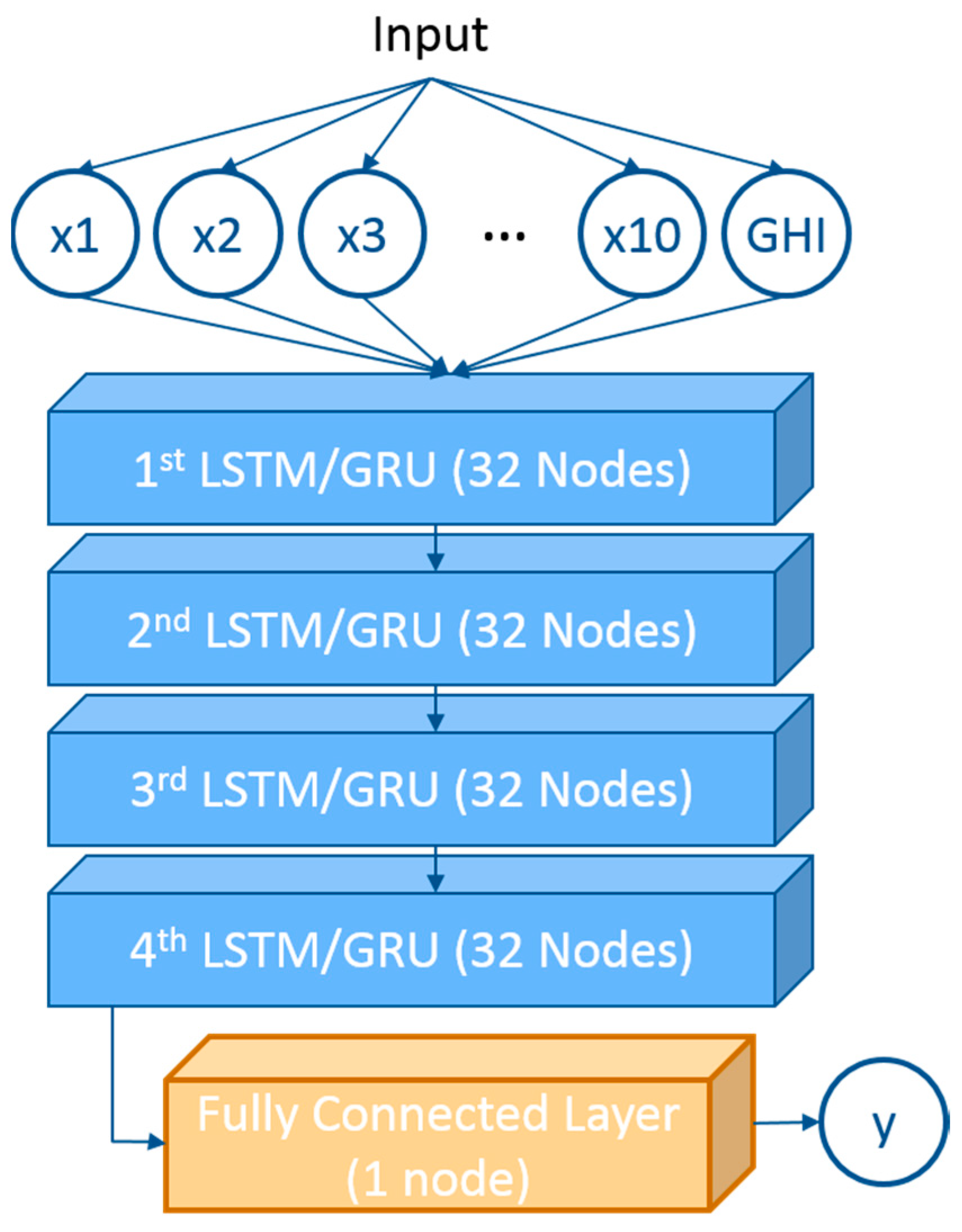
3. Deep Learning Architectures

In this section, FFNN, RNN, LSTM, and GRU architectures are explained with respect to the time series problem, i.e., solar radiation forecasting. Section 3.1 describes the FFNN while Section 3.2 describes the RNN and Section 3.3 explains a comparison of RNN extensions, i.e., LSTM and GRU with respect to time series forecasting.

3.1. Feed Forward Neural Network (FFNN)

It is the simplest form of a deep neural network, used as a reference model. Figure 6a shows a simple example of an FFNN. The input is fed to the hidden layer in the forward direction until the output is calculated using activation functions in each hidden layer node and initialized weights and biases. Later, weights are adjusted using backpropagation algorithm and the loss functions to get optimal values. Figure 6b shows our FFNN model using the Keras and TensorFlow framework. The model consists of an input with 11 entries of historical and GHI data, four hidden layers each with 32 nodes, and an output layer with a single node. As FFNNs are feedforward not feedback; they do not have the mechanism to utilize or remember past outputs, unlike the RNN. Therefore, they are not suited for time series forecasting.

3.2. Recurrent Neural Network (RNN)

As shown in Figure 7a an RNN is an extension of a conventional FFNN, a feedback, which is able to use the last time step output as input at each node. RNN is useful for sequential data as it handles the variable-length sequence by having a recurrent hidden state whose activation at each time is dependent on that of the previous time-step.
An RNN consists of one hidden layer that maintains hidden states and a fully-connected layer to get output from its hidden states. The hidden unit of an RNN unit is shown in Figure 8. The hidden state ht is defined as follows:
h 0 = 0   h t = t a n h ( U x t + W h t 1 )  
where xt is the input to hidden layer, ht–1 is the previous hidden state from the previous time-step, U is the weight matrix for input, and W is the weight matrix for the previous hidden state.
After the hidden state is obtained, RNN output ot is directly calculated from the current hidden state in a fully-connected layer as follows:
o t = σ ( V h t )
where σ is a sigmoid activation function and V is the corresponding output weight.
Unfortunately, it was observed in [39] that it is difficult to train RNNs to capture long-term dependencies because the gradients tend to either most of the time vanish or rarely tend to explode. To solve these issues LSTM unit was introduced, and then gated recurrent units (GRUs) followed LSTM more recently [40]. These two extensions of RNN were shown to solve the issues of gradient by capturing long-term dependencies. The RNN model used in this paper is shown in Figure 7b. This model consists of an input with 11 entries for historical and GHI data, four hidden layers with 32 RNN units in each layer, and a fully connected layer with a single node to predict the solar radiation data.

3.3. LSTM vs. GRU

Unlike the recurrent unit, which simply computes a weighted sum of the input signals and applies a nonlinear function, each LSTM unit maintains one memory at a time. An LSTM unit consists of three gates, i.e., input, output, and forget gates with an internal memory. An LSTM unit is able to decide whether to keep or forget the existing memory via the introduced gates. Intuitively, if the LSTM unit detects an important feature from an input sequence at early stage, it easily carries this information over a long distance, hence, capturing potential long-distance dependencies. A comparison of RNN vs. LSTM vs. GRU units is shown in Figure 8.
The input gate of LSTM decides how much current information needs to be passed according to the following equation:
i t = σ ( x t U i + h t 1 W i ) .
The forget gate decides the information needed to be forgotten from the previous state and is defined as follows:
f t = σ ( x t U f + h t 1 W f ) .
The output gate defines the internal state information that needs to be passed using the following equation:
o t = σ ( x t U o + h t 1 W o ) .
The internal memory, also known as the cell state Ct, is updated in two steps. At first, a candidate of cell state C ˜ t is calculated using the following formula:
C ˜ t = t a n h ( x t U g + h t 1 W g )
where   U g and W g represent each of the weight matrices multiplied to inputs of the cell state operation. After C ˜ t is calculated, the cell state Ct is updated from C ˜ t as follows:
C t = σ ( f t × C t 1 + i t × C ˜ t )
where * is an operation of element-wise multiplication. The cell state Ct is used to obtain the hidden state of the next time-step using the following formula:
h t = t a n h ( C t ) × o t .
Similar to the LSTM unit, the GRU has two gates, namely the reset and update gates, which modulate the flow of information inside the unit without, however, having separate memory cells. The reset gate of the GRU is defined as follows:
r t = σ ( x t U r + h t 1 W r ) .
The update gate output z t is calculated by the following formula:
z t = σ ( x t U z + h t 1 W z ) .
The hidden state of GRU h t is updated in two steps. Firstly, the temporary output of the hidden state from the reset gate is calculated as h ˜ t . After that, h t is calculated with the update gate output z t as follows:
h ˜ t = tanh ( x t U h + ( r t × h t 1 ) W h ) h t = ( 1 z t ) × h t 1 + z t × h ˜ t .
The GRU is similar to LSTM in terms of remembering important information and carrying it to long distances, capturing long-term dependencies. It is computationally more efficient with less complexity. It is observed to perform faster and better than LSTM on certain data. The LSTM and GRU models used in this paper are shown in Figure 9.

4. Experiment and Results

Real-time hourly and daily solar radiation data was obtained from the Korea Meteorological Administration (KMA) for Seoul and Busan regions in South Korea. The two regions were selected considering their geographical differences. As shown in Figure 10, Seoul is in the northern part of Korea surrounded by mountains while Busan is located at the southern coastline of the country.
As discussed in the data selection section, for both regions, historical hourly and daily solar radiation data from 2000 to 2016 were used to train the model along with clear sky GHI data, while 2017 hourly and daily solar radiation were predicted, respectively. Different deep learning models were implemented and compared to achieve this objective. The models compared were the state of the art models: SVR, RNN, FFNN, LSTM, and GRU. Comparison of the proposed models with the state of the art traditional method, i.e., RFR was also made. The models were implemented in Python using a Jupyter Notebook with Keras and TensorFlow at the back-end. The error criteria used in this paper was root mean square error (RMSE).

Results

Table 2 and Table 3 show the comparison of RMSE for hourly and daily periods. Training data from 2000 until 2015 and corresponding clear sky GHI data were used to predict data from 2016. Similarly, data from 2000 to 2016 with corresponding clear sky GHI data were used to predict 2017 data.
Table 4 and Table 5 show performance of LSTM and GRU models. The performance was measured as training time in a system with an AMD Ryzen Threadripper 2950X and 64 GB RAM, and only a CPU was used for model fitting and prediction. The measurements were mean values taken from 10 runs for accurate results. Table 6 compares total radiation of each model for one year ahead.
Figure 11 shows absolute values of prediction errors for each model in the perspective of total yearly radiation. The lower value indicates that it is more similar to the actual data.
Figure 12 and Figure 13 show comparisons of actual data vs. standard RNN and its extensions (i.e., LSTM, GRU) trained with the training data until year 2016, for the prediction of year 2017 in monthly time steps for two regions, respectively.

5. Discussion

The discussion can be divided into two parts: accuracy comparison and performance comparison.

5.1. Comparison of Accuracy

In this paper, the proposed deep learning-based methods, specifically LSTM and GRU, were compared with the state of the art traditional method (RFR) [12]. In Table 2 and Table 3, comparisons of hourly and daily one year ahead solar radiation forecasting are shown. As can be seen from these tables, the proposed model is far better compared to the traditional method. The reason for better performance of LSTM and GRU compared to the traditional method is due to its inherent characteristics of carrying initially learnt important information over a long distance [39,40]. Similarly, Table 6 shows the comparison of total radiation for one year ahead. In this table, the proposed models outperformed the traditional approach again.
Comparison among different deep learning models is also made to show the effectiveness of each model. From Table 2 and Table 3, it can be seen that LSTM and GRU is relatively better compared to other models in terms of model accuracy due to their controlling gates and memory of long-term dependencies. It is generally recognized that LSTM and GRU are similar and only show different performance depending on the nature of problem, data features, and size. However, on our dataset, GRU performed marginally better than LSTM. Similarly, Table 6 and Figure 11 show the accuracy of each model for total one year ahead solar radiation forecasting. GRU is relatively better compared to other models. Figure 12 and Figure 13 show the comparison of RNN and its extensions, i.e., LSTM and GRU, for one year ahead solar radiation in monthly period.
As the experimental results shows, our proposed approach reached a new state of the art in terms of accuracy. We expect our work to be useful in different kinds of applications like microgrid simulation design, installation, and planning. Furthermore, it can be applied in the estimation of degradation-rate-influenced energy potentials of PV panels.

5.2. Comparison of Performance

Comparison of performance of the two most effective and state of the art deep learning models, i.e., LSTM vs. GRU, is shown in Table 4 and Table 5. As discussed above, GRU has two gates compared to LSTM, which has three gates, which results in reducing the complexity of the structure. Therefore, less operation is needed for GRU compared to LSTM; hence, GRU shows much better performance.
Since GRU has a smaller performance cost, and it is expected that GRU is more applicable in performance-critical environments such as embedded devices like intelligent electronic devices (IEDs) in smart grids.

6. Conclusions

For microgrid design and engineering, it is necessary to estimate renewable generation capacity, energy storage system (ESS) capacity, total demand, simulation capacities, etc. For these purposes, very long-term generation and demand need to be forecasted. Solar power generation forecasting mainly depends on the amount of solar radiation. Therefore, long-term solar radiation is required to be forecasted. Long-term solar radiation forecasting is also necessary for the estimation of the degradation-rate-influenced energy potentials of PV panels. Traditionally probabilistic approaches are used for long-term solar radiation forecasting. However, due to uncertainty from probability based randomness, these approaches are less accurate. In previous works, machine learning algorithms like RFR were also being used. In this work, we applied the deep learning-based approach to predict long term solar radiation due to its huge success in diverse fields including time series forecasting.
Historical solar radiation data and clear sky GHI data predicted from the most suitable clear sky GHI model were used as input data. Different state of the art machine learning (ML) and deep learning (DL) approaches were applied and compared. The models compared were traditional methods like RFR and SVR and state of the art deep learning models such as FFNN, RNN, LSTM, and GRU. The deep learning models outperformed the traditional methods in terms of model accuracy. Among the deep learning models, LSTM and GRU were better than others due to their characteristics of carrying important information over a long distance. Among two of them, GRU showed slightly better results compared to LSTM. In addition to model accuracy, the performance of two state of the art deep learning models, LSTM and GRU, was also measured. Among them, GRU performed relatively faster due to its fewer gates than LSTM. From these observations, we proposed LSTM and GRU as promising deep learning-based approaches for long-term solar radiation forecasting.
With respect to long-term solar radiation forecasting, since our proposed approach reached a new state of the art in terms of accuracy, we expect our work can be applied to different kind of applications. Precisely, predicted one year ahead hourly and daily data can be used for the following purposes: Firstly, as discussed above, it can be used for simulation design, installation, and planning of renewables, especially in microgrids. Secondly, this yearly ahead data can be used to study the degradation-rate-influenced energy potentials of PV panels. Thirdly, meteorological departments can take help from predicted data to carry out weather-related research. Additionally, it has been found that GRU is more suitable for performance-critical environments like IEDs in smart grids since GRU has the smallest calculation cost.

Author Contributions

M.A. and J.-M.L. are the main authors and contributed equally to this work. They together designed and implemented the simulations and wrote the paper. S.H. and S.-J.L. supervised and gave their valuable ideas to improve the results. H.-S.K. supported discussions on improvements and carried out proof reading of the article. All authors have read and agreed to the published version of the manuscript.

Funding

This work was supported by the “Human Resources Program in Energy Technology” of the Korea Institute of Energy Technology Evaluation and Planning (KETEP), and was granted financial resources from the Ministry of Trade, Industry and Energy, Republic of Korea. (No. 20174030201790). This research was supported by the Korea Electric Power Corporation (Grand number: R18XA01).

Acknowledgments

Thank you to Myongji University, Yongin, Korea and the Next-Generation Power Technology Center, Yongin, Korea, for their logistic support.

Conflicts of Interest

The authors declare no conflict of interest.

References

  1. Sare, C.B.; Paul, R.M. Peaceful coexistence: Independent microgrids are coming. In Public Utilities Fortnightly; University of Connecticut: Reston, VA, USA, 2013; Available online: https://works.bepress.com/bronin/ (accessed on 14 December 2019).
  2. Carpintero-Rentería, M.; Santos-Martín, D.; Guerrero, J.M. Microgrids Literature Review through a Layers Structure. Energies 2019, 12, 4381. [Google Scholar] [CrossRef] [Green Version]
  3. Manzoor, E.; Ghulam, A.; Irfan, K.; Paul, M.K.; Mashood, N.; Ali, R.; Umar, F. Recent approaches of forecasting and optimal economic dispatch to overcome intermittency of wind and photovoltaic (PV) systems: A review. Energies 2019, 12, 4392. [Google Scholar]
  4. Sawin, J.L.; Sverrisson, F.; Rutovitz, J.; Dwyer, S.; Teske, S.; Murdock, H.E.; Adib, R.; Guerra, F.; Blanning, L.H.; Hamirwasia, V. Renewables 2018 Global Status Report; REN21: Pairs, France, 2018. [Google Scholar]
  5. Jeff, L.; Michael, G.; Matt, G. The Importance of Wind Forecasting—Renewable Energy Focus. Available online: http://www.renewableenergyfocus.com/view/1379/the-importance-of-wind-forecasting (accessed on 14 December 2019).
  6. Tim, J.; Florian, S. Forecasting the price distribution of continuous intraday electricity trading. Energies 2019, 12, 4262. [Google Scholar]
  7. Inman, R.H.; Pedro, H.T.C.; Coimbra, C.F.M. Solar forecasting methods for renewable energy integration. Prog. Energy Combust. Sci. 2013, 39, 53–576. [Google Scholar] [CrossRef]
  8. Hussain, A.; Arif, S.M.; Aslam, M. Emerging renewable and sustainable energy technologies: State of the art. Renew. Sustain. Energy Rev. 2017, 71, 12–28. [Google Scholar] [CrossRef]
  9. Nouha, M.; Abderezak, L.; Dezso, S.; Josep, M.G.; Adnen, C. Large photovoltaic power plants integration: A review of challenges and solutions. Energies 2019, 12, 3798. [Google Scholar]
  10. Kim, H.S.; Aslam, M.; Choi, M.S.; Lee, S.J. A study on long-term solar radiation forecasting for PV in microgrid. In Proceedings of the APAP Conference, Jeju, Korea, 16–19 October 2017. [Google Scholar]
  11. Peder, B.; Henrik, M.; Henrik, A.N. Online short-term solar power forecasting. Sol. Energy 2009, 83, 1772–1783. [Google Scholar]
  12. Nallpaneni, M.K.; Subarthra, M.S. Three years ahead solar radiation forecasting to quantify degradation influenced energy potentials from thin film (a-Si) photovoltaic system. Results Phys. 2019, 12, 701–703. [Google Scholar]
  13. Phathutshedzo, M.; Caston, S.; Alphonce, B.; Sophie, M. Day ahead hourly global horizontal irradiance forecasting-approach to south African data. Energies 2019, 12, 3569. [Google Scholar]
  14. Rezaie-Balf, M.; Maleki, N.; Kim, S.; Ashrafian, A.; Babaie-Miri, F.; Kim, N.W.; Chung, I.M.; Alaghmand, S. Forecasting daily solar radiation using CEEMDAN decomposition-based MARS model trained by crow search algorithm. Energies 2019, 12, 1416. [Google Scholar] [CrossRef] [Green Version]
  15. Antonanzas, J.; Osorio, N.; Escobar, R.; Urraca, R.; Martinez-de-Pison, F.J.; Antonanzas-Torres, F. Review of photovoltaic power forecasting. Sol. Energy 2016, 136, 78–111. [Google Scholar] [CrossRef]
  16. Ahmed, A.; Khalid, M. A review on the selected applications of forecasting models in renewable power systems. Renew. Sustain. Energy Rev. 2019, 100, 9–21. [Google Scholar] [CrossRef]
  17. Abuella, M.; Chowdhury, B. Solar Radiation Probabilistic Forecasting by Using Multiple Linear Regression Analysis. In Proceedings of the SoutheastCon 2015, Fort Lauderdale, FL, USA, 9–12 April 2015. [Google Scholar]
  18. Sobrina Sobri, S.; Koohi-Kamali, S.; Rahima, N.A. Solar photovoltaic generation forecasting methods: A review. Energy Convers. Manag. 2018, 156, 459–497. [Google Scholar] [CrossRef]
  19. Miller, S.D.; Rogers, M.A.; Haynes, J.M.; Sengupta, M.; Heidinger, A.K. Short-term solar radiation forecasting via satellite/model coupling. Sol. Energy 2018, 168, 102–117. [Google Scholar] [CrossRef]
  20. Huang, J.; Perry, M. A semi-empirical approach using gradient boosting and k-nearest neighbors regression for gefcom2014 probabilistic solar radiation forecasting. Int. J. Forecast. 2016, 32, 1081–1086. [Google Scholar] [CrossRef]
  21. Alessandrini, S.; Monachel, D.; Sperati, S.; Cervone, G. An analog ensemble for short-term probabilistic solar radiation forecast. Appl. Energy 2015, 157, 95–110. [Google Scholar] [CrossRef] [Green Version]
  22. Philipp, L.; Mathieu, D.; Hugo, T.C. Probabilistic solar forecasting using quantile regression models. Energies 2017, 10, 1591. [Google Scholar]
  23. Min, K.B.; Duehee, L. Spatial and temporal day-ahead total daily solar radiation forecasting: Ensemble forecasting based on the empirical biasing. Energies 2018, 11, 70. [Google Scholar]
  24. Yang, D.; Ye, Z.; Lim, L.H.I.; Dong, Z. Very short term radiation forecasting using the lasso. Sol. Energy 2015, 114, 314–326. [Google Scholar] [CrossRef] [Green Version]
  25. Wang, F.; Zhen, Z.; Wang, B.; Mi, Z. Comparative study on KNN and SVM based weather classification models for day ahead short term solar PV power forecasting. Appl. Sci. 2018, 8, 28. [Google Scholar] [CrossRef] [Green Version]
  26. Zhenyu, W.; Cuixia, T.; Qibling, Z. Hourly solar radiation forecasting using a Volterra-least squares support vector machine model combined with signal decomposition. Energies 2018, 11, 1138. [Google Scholar] [CrossRef] [Green Version]
  27. Ariana, M.; Walter, R.; Rolando, V.A. Deep Learning to forecast solar radiation using a six-month UTSA SkyImager dataset. Energies 2018, 11, 1988. [Google Scholar]
  28. Munir, H.; Il-Yop, C. Day-ahead solar radiation forecasting for microgrids using a long-short term memory recurrent neural network: A Deep Learning approach. Energies 2019, 12, 1856. [Google Scholar]
  29. Jessica, W.; Matin, H.; Raju, G.; Terrence, L.C. Hour-ahead solar radiation forecasting using multivariate gated recurrent units. Energies 2019, 12, 4055. [Google Scholar]
  30. Rahul, A.; Frankle, M.; Madan, T. Long term load forecasting with hourly predictions based on long-short-term-memory networks. In Proceedings of the IEEE Texas Power and Energy Conference (TPEC), College Station, TX, USA, 8–9 February 2018. [Google Scholar]
  31. Mustafa, A.; Nejat, Y. Year ahead demand forecast of city natural gas using seasonal time series data. Energies 2016, 9, 727. [Google Scholar]
  32. John, G. Deep Learning for Time-Series Analysis. arXiv 2017, arXiv:1701.01887. Available online: https://arxiv.org/abs/1701.01887 (accessed on 14 December 2019).
  33. Korea Meteorological Administration. Available online: https://web.kma.go.kr/eng/index.jsp (accessed on 14 December 2019).
  34. Bird, R.E.; Hulstrom, R.L. Simplified Clear Sky Model for Direct and Diffuse Insolation on Horizontal Surfaces; Solar Energy Research Inst.: Golden, CO, USA, 2013; pp. 1–38. [Google Scholar]
  35. Manajit, S.; Peter, G. Evaluation of Clear Sky Models for Satellite-Based Irradiance Estimates; Technical Report of National Renewable Energy Laboratory (NREL): Denver West Parkway, CO, USA, 2013; pp. 5–29. [Google Scholar]
  36. Ineichen, P.; Perez, R. A new airmass independent formulation for the Linke turbidity coefficient. Sol. Energy 2002, 73, 151–157. [Google Scholar] [CrossRef] [Green Version]
  37. Haurwitz, B. Insolation in relation to cloudiness and cloud density. J. Meteorol. 1945, 2, 154–166. [Google Scholar] [CrossRef]
  38. Ineichen, A. Broadband simplified version of the Solis clear sky model. Sol. Energy 2008, 82, 758–762. [Google Scholar] [CrossRef] [Green Version]
  39. Bengio, Y.; Simard, P.; Frasconi, P. Learning long-term dependencies with gradient descent is difficult. IEEE Trans. Neural Netw. 1994, 5, 157–166. [Google Scholar] [CrossRef]
  40. Cho, K.; van Merriënboer, B.; Bahdanau, D.; Bengio, Y. On the properties of neural machine translation: Encoder-decoder approaches. arXiv 2014, arXiv:1409.1259. Available online: https://arxiv.org/abs/1409.1259 (accessed on 14 December 2019).
  41. Surabh, R. Medium: Simple RNN vs. GRU vs. LSTM: Difference Lies in More Flexible Control. Available online: https://medium.com/@saurabh.rathor092/simple-rnn-vs-gru-vs-lstm-difference-lies-in-more-flexible-control-5f33e07b1e57 (accessed on 14 December 2019).
Figure 1. Microgrid installation and revenue generation.
Energies 13 00147 g001
Figure 2. Participation of renewables in microgrid.
Energies 13 00147 g002
Figure 3. Clear sky GHI and observed radiation.
Energies 13 00147 g003
Figure 4. Correlation between observed GHI (Y) vs. historical data (X) and clear sky GHI.
Energies 13 00147 g004
Figure 5. Input data to the model for training and testing.
Energies 13 00147 g005
Figure 6. FFNN model: (a) an example of FFNN; (b) our FFNN model.
Energies 13 00147 g006
Figure 7. RNN model: (a) simple RNN; (b) our RNN model.
Energies 13 00147 g007
Figure 8. Comparison of RNN vs. LSTM vs. GRU units [41].
Energies 13 00147 g008
Figure 9. The LSTM/GRU model.
Energies 13 00147 g009
Figure 10. Geographical difference of the two selected regions.
Energies 13 00147 g010
Figure 11. Absolute errors of trained models in total yearly radiation.
Energies 13 00147 g011
Figure 12. Comparison of RNN and its extensions in monthly time steps for Seoul Region.
Energies 13 00147 g012
Figure 13. Comparison of RNN and its extensions in monthly time steps for Busan Region.
Energies 13 00147 g013
Table 1. RMSE for different clear sky GHI models.
ML 1/DL 2 ModelIneichen and PerezBirdHaurwitzSimplified Solis
SVR0.39950.39900.39910.3991
RFR0.41210.41120.41030.4102
FFNN0.39100.39360.39310.3943
RNN0.40420.40090.40110.4038
LSTM0.39080.38980.38970.3881
GRU0.39040.38700.39130.3892
Best0.39040.38700.38970.3881
Worst0.41210.41120.41030.4102
Mean0.39800.39690.39740.3974
1 machine learning, 2 deep learning.
Table 2. RMSE of hourly solar radiation for different models.
RegionYearSVRRFRFFNNRNNLSTMGRU
Seoul20170.39900.40990.39280.40520.39200.3909
20160.37920.38630.36330.37900.35960.3598
Busan20170.43120.43920.42290.43520.41780.4134
20160.48980.48700.46860.47170.46050.4582
Table 3. RMSE of daily solar radiation for different models.
RegionYearSVRRFRFFNNRNNLSTMGRU
Seoul20175.36185.67055.44926.02005.36965.3315
20164.81595.12015.11035.45204.77684.8233
Busan20175.74985.94095.83186.27185.57525.6372
20166.64016.90866.58906.77596.31656.2672
Table 4. Performance of LSTM vs. GRU hourly data.
RegionYearLSTM (seconds)GRU (seconds)
Seoul20171251.231004.15
20161060.82832.63
Busan20171269.211028.43
20161023.27830.54
Table 5. Performance of LSTM vs. GRU daily data.
RegionYearLSTM (seconds)GRU (seconds)
Seoul201788.3572.56
201677.9864.12
Busan201790.4275.44
201675.9964.29
Table 6. Total yearly radiation.
RegionYearActual (MJ/m2)SVR (MJ/m2)RFR (MJ/m2)FFNN (MJ/m2)RNN (MJ/m2)LSTM (MJ/m2)GRU (MJ/m2)
Seoul20174577.294729.334326.264274.164309.464430.234443.65
20164520.885154.554377.964295.384018.724450.804422.67
Busan20175418.946113.095029.505154.515370.555438.855426.70
20165025.295733.475331.145387.455315.515222.495098.98

