Adaptive Backstepping Nonsingular Fast Terminal Sliding Mode Control for Hydro-Turbine Governor Design

Abstract

To investigate a typical large-scale nonlinear hydropower system (HS) with a stochastic water flow, a novel nonlinear adaptive control scheme, which is created by the combination of a backstepping strategy, nonsingular fast terminal sliding mode surface and command filter, is proposed for the hydro-turbine governor design of a HS to not only improve the transient stability of the HS but also increase the energy conversion efficiency and improve the reliability and availability of the electricity supply. In contrast to previous research based on ideal hydro-turbine models with accurate parameters, an adaptive backstepping nonsingular fast terminal sliding mode control (ABNFTSMC) with command filtered (CF) is proposed in which virtual control inputs and error compensations are applied to overcome distribution characteristics resulting from energy losses, while guaranteeing finite-time convergence. In addition, to avoid the requirement of analytic differentiation in Lyapunov stability, a command filter method is used to generate certain compensating signals and their derivatives. In this paper, the Nazi Gorge hydropower station in China is used as our verification model of a hydropower plant with monitored data, where energy losses and random water flow disturbances are considered. Simulation results illustrate that the proposed control strategy for a hydro-turbine governor can significantly increase the stability, reliability, and system performance of a HS even in the presence of uncertainties.

1. Introduction

In recent years, with the request to improve the quality of life and human health and the desire to reduce global warming, the demand for renewable energy has increased significantly. Thus, one of the most important challenges currently is enhancing the impact of renewable energy in existing power systems. Up to now, hydropower power generation is still the most effective large-scale method of electricity production [1,2,3,4,5,6]. The energy flows are centralized and can easily be controlled, and in addition, the kinetic energy of the conversion process can be directly converted into electrical energy without heat loss or any chemical processes. Currently, due to the development of large interconnected hydropower system (HS), novel design architectures and equipment, HS has become increasingly diverse and challenging, especially in size and complexity. Figure 1 illustrates the basic schematic of HS. The operation process of HS is mainly based on the high ground difference between the reservoir and the power plant to guide the high-level water stored in the high mountain reservoirs and lakes to the hydraulic power at a low level through the water diversion pipe system. There are two main parts in HS, i.e., hydro-turbine and generator. A hydro-turbine is much like a windmill, except the energy is provided by water flow instead of wind. The turbine converts the kinetic energy of water flow into mechanical energy. Connected to the turbine, the generator spins also to converts the mechanical energy from the turbine into electric energy. Thereby, the hydropower plant could provide electricity to homes and businesses by transmission lines.

The conversion efficiency of a HS, which primarily depends on the type of hydro-turbine governor, is a key performance indicator to evaluate the utilization factor. The hydro-turbine governor obtains information regarding the current angular speed for the generator. Thus, it regulates the inlet of water into the turbine to maintain the speed at the correct level and then enables the rotation of the generator to produce electricity with a stable power supply. Therefore, the hydro-turbine governor is really important in a HS, which has a direct impact on the stability of the hydropower station and power grid systems. Nevertheless, because of a complicated multivariable nonlinear system exhibiting parametric uncertainty and unknown nonlinear disturbances, to control the hydro-turbine governor is a big challenge. Hence, minimizing the impact of disturbances on the operation of the power system and on the power system balance and control is particularly important.

To ameliorate the transient stability of a HS and to enhance their power conversion efficiency and electricity productivity, the governor control system must be considered. Recently, numerous studies have evaluated control schemes for hydro-power systems, which have improved governor control system reliability; for example, see [7,8,9] and the references therein. An adaptive backstepping-based control scheme frequently utilized to address nonlinear uncertain systems [10,11]. However, the traditional backstepping scheme has a drawback which is the complexity resulting from repeated differentiation [12]. Li et al. [13] proposed a robust adaptive control in which the backstepping method is combined with a robust disturbance attenuation technique to ensure that the closed-loop system is globally bounded. In [14], Cai et al. used a direct fuzzy backstepping method to design a control for a nonlinear power system. Fuzzy logic systems are utilized to approximate unknown power system functions, and then the stability of the system is guaranteed by the Lyapunov theory. Su et al. [15] proposed an adaptive backstepping sliding mode control (ABSMC) scheme for solving the nonlinear system problem with unknown bounded uncertainties. However, the traditional sliding mode control (SMC) cannot provide a finite-time convergence; in addition, this scheme cannot effectively handle rapid variation effects resulting from disturbances and/or faults although it has a good transient response in normal operation. To ensure finite-time convergence, a terminal SMC has been proposed [16,17,18]. The advantages of terminal SMC include faster finite-time convergence and higher control precision; however, an intrinsic singularity problem arises in terminal SMC due to the use of fractional power functions as the sliding hyperplane. To overcome the above problems, a rapid terminal SMC and a nonsingular terminal SMC have been developed. However, for high-order nonlinear systems, the problem of increasing complexity arises, caused by repeated differentiations of certain nonlinear functions and virtual controls in the Lyapunov stability analysis. To overcome this drawback, the CF backstepping approach was introduced in [19] to eliminate the need for analytic computation of the time derivatives of virtual errors.

In this paper, a hydro-turbine governor for speed control based on varying positions of the guide vanes is designed for a large-scale HS, which employs an adaptive backstepping nonsingular fast terminal sliding mode control (ABNFTSMC) a CF; this governor is based on an actual HS, i.e., the Nazixia hydropower station in China. First, a dynamic eight-order hydropower plant model, including a hydro-turbine governor control unit and a generator control unit, is established while considering a stochastic water flow and the distribution characteristics of energy losses of a HS. Second, to address the effects of energy losses from a stochastic turbine flow and to increase the energy conversion efficiency, i.e., to improve the reliability and availability of the electricity supply, ABNFTSMC approach is utilized; meanwhile, by introducing a CF to approximate the derivative of the virtual control, the problem of increasing complexity can be resolved. Additionally, the proposed control scheme can ensure finite-time convergence without a singularity; the scheme also exhibits a fast transient response, high precision tracking, and a guaranteed global asymptotic stability. The primary contributions of this paper can be summarized as follows:

(1)

An actual and complete HS model is established, based on the Nazi Gorge hydropower station in China, which considers internal energy losses due to a stochastic water flow. The internal energy losses include both hydraulic and electrical losses.

(2)

An adaptive backstepping control strategy combined with nonsingular fast terminal sliding mode control is employed to obtain the control output of an eight-order nonlinear HS with a stochastic water flow to ensure finite-time convergence without a singularity as well as a fast transient response, high tracking performance, and global asymptotic stability.

(3)

By incorporating a CF, the analytical derivative is unnecessary; thus, the problem of increasing complexity in the backstepping control procedure can be avoided. Moreover, a nonsingular fast terminal sliding mode surface is used to construct a finite-time CF such that each subsystem can ensure rapid finite-time convergence without a singularity.

(4)

Compared with the traditional ABSMC method [15], the proposed approach exhibits superior performance. For instance, the mechanical power of the hydro-turbine and the electrical power of generator increase by 376 and 740 kW; respectively, and the effectiveness of the mechanical power of the hydro-turbine increases by 1.06% for a stochastic intensity of 0.6. At the same time, the overall energy loss is effectively reduced by 600 kW compared with the ABSMC scheme [15] for a stochastic intensity of 0.6.

2. Mathematical Modeling of a HS with Energy Losses

Hydropower is currently the most important and economical type of renewable, sustainable energy, in which the energy of falling water is converted into electricity. A component diagram of a HS is shown in Figure 2.

The HS includes two components, i.e., a hydro-turbine governor control unit and a generator control unit. For the hydro-turbine governor control unit, the water first flows through the water valve (WV) into the penstock system (PS), also commonly known as the penstock pipe; then, the stay ring (SR) directs water from the turbine scroll (TS) casing to the guide vane (GV). Thus, kinetic energy and potential energy can be generated in the water as the hydro-turbine begins to rotate. The turbine governor controller (TGC) primarily controls the GV position for the turbine governor. The generator control unit consists of a drive system (DS), automatic voltage regular (AVR), and power system stabilizer (PSS), where E is the excitation, $\Phi$ is the magnetic field, G is the generator and TCSC is a thyristor-controlled series capacitor. The hydro-turbine drives the generator rotor rotation such that the mechanical energy is converted into electrical energy, which is fed into the electricity grid system. Note that the TGC controls the amount of water entering the turbine via the GV and therefore controls the efficiency of the mechanical power. The hydro turbine is a device that transfers the energy from the moving water to the GV to generate electricity. The PSS and AVR are dynamically interlinked to lead additional signals ahead of the power angle and speed such that the generator output terminal voltage is automatically maintained at a set value under varying loads and operating temperatures. The output is controlled as the voltage at a power-generating coil is compared with a stable reference. An error signal is used to adjust the average value of the field current. In Figure 2, HL, ML, and EL respectively indicate the hydraulic loss, the mechanical loss, and the electrical loss. $q_0$ is the rated water flow, $y_0$ is the rated GV opening, ${\delta }_0$ is the rated rotor angle, ${\omega }_0$ is the rated angular speed, and $E_{q_o}$ is the rated terminal voltage.

2.1. Hydro-Turbine Governor Control Unit

The hydro-turbine governor unit is primarily used to convert the water flow into mechanical power and is composed of a PS, hydro-turbine, spiral case, GV, and governor. The PS acts as a conveying pipe to convey water from the reservoir to the turbine. In addition, the governor is used to automatically adjust the opening distance of the GV in the turbine to adjust the water flow and the head height difference; hence, the governor can increase the effective utilization rate of the water flow and the turbine efficiency, thus directly affecting the entire HS. However, in the process of transportation, this process is inevitably affected by the stochastic water flow in the external reservoir, and the hydraulic loss in the pipes causes the flow velocity to decrease. Therefore, when designing the PS, one must consider the influence of the changing water flow in the pipes, including the hydraulic losses for the water flow and the hydro-turbine. According to Reference [8,20,21], the nonlinear model of the hydro-turbine governor control unit can be expressed as Equation (1), where $q$ is the relative water flow for the hydro-turbine, $y$ is the relative derivative of the GV opening for the hydro-turbine, and $u_y$ is the control signal of the hydro-turbine governor. $T_0$, $Z_0$, $T_y$ denote the penstock elastic constant, the impedance coefficient of the hydraulic surge, and the elastic constant of the hydro-turbine respectively; $h_0$ is the gross head of the HS, and $h_{loss}$ is the hydraulic loss of the penstock, which can be expressed as $h_{loss}=f_q{q}^2$ where $f_q$ is the friction factor of the penstock. $y_0$ and $y_r$ refer to the initial incremental deviation and the incremental deviation of the GV.

$$\begin{array}{l}{\dot{x}}_1=x_2,\\ {\dot{x}}_2=x_3,\\ {\dot{x}}_3=-\frac{{\pi }^2}{T_0^2}{x}_2+\frac{1}{Z_0{T}_0^3}\left(h_0-h_{loss}-\frac{y_r^2}{y^2}{q}^2\right),\\ \dot{q}=-3{\pi }^2{x}_2+\frac{4}{Z_0{T}_0}\left(h_0-h_{loss}-\frac{y_r^2}{y^2}{q}^2\right),\\ \dot{y}=\frac{1}{T_y}\left(u_y-y-y_{\mathrm{o}}\right)\end{array}$$

(1)

2.2. Generator Control Unit

Hydropower station is generally designed to provide flow regulation in order to maximize the electricity generation where the hydraulic turbine converts the energy of flowing water into mechanical power and then produces electricity via generators driven by turbines. The operation of the hydropower generator is primarily affected by the power angle and the relative deviation of the angular speed for the generator, which both influence the electrical power output of the entire HS. To ensure the optimum generation of electricity, a system composed of an AVR [22], PSS [23] and TCSC [24] is used in the generator control unit as the basis for adjusting the voltage of the exciter to ensure that the entire HS produces high quality electrical power. The mathematical model of the generator control unit can be given as:

$$\begin{array}{l}\dot{\delta }={\omega }_B\left(\omega -1\right),\\ \dot{\omega }=\frac{1}{T_j}\left(P_m-P_e-D_t\left(\omega -1\right)\right),\\ {\dot{E}}_q=-\frac{{\omega }_B}{T_{d0}}\frac{X_d{E}_q}{X_{d0}}+\frac{{\omega }_B}{T_{d0}}\frac{X_d-X_{d0}}{X_{d0}}{V}_s\cos \delta +\frac{{\omega }_B{E}_f}{T_{d0}}\end{array}$$

(2)

where $\delta$ is the rotor angle relative deviation for the generator; $T_j$ is an inertial time constant; ${\omega }_B$ and $\omega$ are the base value and the relative deviation of the angular speed respectively; $P_m$, $P_e$, $D_t$ denote the mechanical power of the hydro-turbine, the electrical power of the generator, and the damping coefficient of generator; $E_q$ is the internal transient voltage, $X_d$ is the d-axis reactance, $X_{d0}$ is the d-axis transient reactance, $T_{d0}$ is a time constant, $V_s$ is the voltage of the generator, and $E_f$ is the voltage control for a single generator. The electrical power of the generator $P_e$ can be expressed as:

$$P_e=\frac{E_q{V}_s\sin \delta }{X_{d0}}+\frac{V_s^2\left(X_d{}_0-X_q\right)}{2X_{d0}{X}_q}\sin 2\delta$$

(3)

where $X_q$ denotes the q-axis reactance.

Remark 1.

The conversion efficiency of the generator can be indicated as:

$$C{E}_g={P_m/P}_e$$

(4)

which indicates that the generator has an optimal efficiency when, corresponding to a minimum energy loss.

Remark 2.

In general, a turbine converts the kinetic energy of falling water into mechanical power. However, the process of energy conversion always involves a loss of usable energy. The internal energy losses of a hydro-turbine can generally be divided into hydraulic losses, volume losses, and mechanical friction losses. In this paper, we assume that there is no mechanical friction loss, i.e., the energy transfer between the rotating runner of the turbine and fluid is equal to the shaft work. In light of this assumption, the mechanical power of the hydro-turbine can be further expressed as:

$$P_m=P_{input}-P_h-P_v-P_f$$

(5)

where$P_{input}$is the kinetic energy of the input water,$P_v$is the volume loss of the hydro-turbine,$P_h$is the hydraulic loss for the spiral case and$P_f$is the mechanical loss. These energy losses will be explained in detail in the next section.

Remark 3.

The conversion efficiency of the hydro-turbine can be indicated as:

$$C{E}_t={P_m/}_{P_{input}}$$

(6)

2.3. Energy Losses

In order to evaluate the utilization ratio of a HS, one of the most important index is the conversion efficiency. Despite the relatively high work efficiencies of the individual hydraulic elements, the hydraulic operation is not substantially more efficient in terms of energy transformation. The efficiency is generally affected by internal energy losses and stochastic water flow perturbations. The process of energy conversion for a HS is illustrated in Figure 3, where the internal energy losses consist of the hydraulic friction loss of the straight penstock, the hydraulic friction loss for the spiral case, the hydraulic impact loss for the spiral case, the hydraulic loss of the penstock at the inlet for the spiral case, the volume loss, and the hydraulic loss at the SR. The stochastic change in the turbine flow influences these hydraulic losses and thus directly affects the conversion efficiency of the hydro-turbine due to the stochastic water flow. When a hydro-turbine generator operates at low efficiency for a long time, it will affect the conversion efficiency of the HS, and additionally cause serious cavitation erosion and the strong vibrations, thus threatening the safety and stability of the HS.

• Hydraulic Losses

The hydraulic loss for the spiral case is considered as:

$$P_h=\gamma q{h}_w$$

(7)

where $\gamma$ denotes the water density, $q$ is the relative deviation of the hydraulic turbine flow, and $h_w$ is the hydraulic loss for the spiral case [25], which can be written as:

$$h_w=h_{wz}+h_{ww}+h_{wj}$$

(8)

Here, h_wz is the hydraulic friction loss of the straight pipe at the inlet of the spiral case, $h_{ww}$ is the hydraulic friction loss in the spiral case, and $h_{wj}$ is the local hydraulic loss at the SR. Considering the characteristics of a straight penstock, such as the internal penstock pipe friction coefficient, length, and diameter, the hydraulic friction loss $h_{wz}$ can be described as.

$$h_{wz}=\frac{\lambda l}{d}\frac{v_{sp}^2}{2g}$$

(9)

where $\lambda$ is the hydraulic friction loss coefficient, $l$ and $d$ are the length, and the diameter of the penstock pipe, and $v_{sp}$ is the water flow speed in the straight penstock. Moreover, the hydraulic loss for the spiral case $h_{ww}$ [26] can be presented as:

$$h_{ww}=h_{ww1}+h_{ww2}$$

(10)

where $h_{ww1}={\displaystyle {\int }_0^{{\phi }_0}\left(\raisebox{1ex}{$\lambda K^{2}c$}\!\left/ \!\raisebox{-1ex}{$8gF$}\right.\right)}\left(\raisebox{1ex}{$\phi $}\!\left/ \!\raisebox{-1ex}{$2\pi $}\right.\right)d\phi$ is the hydraulic friction loss for the spiral case and $h_{ww2}=\left(\raisebox{1ex}{$1$}\!\left/ \!\raisebox{-1ex}{${\phi }_0$}\right.\right){\displaystyle {\int }_0^{{\phi }_0}{\xi }_{sc}\left(\raisebox{1ex}{$v_{sc}^2$}\!\left/ \!\raisebox{-1ex}{$2g$}\right.\right)}d\phi$ is the impact loss when the water flow impacts the spiral case. $F$ is the cross section of the spiral case, ${\xi }_{sc}$ is the hydraulic impact loss, $v_{sc}$ is the speed of the water flow across the cross-section area $K$ and $c$ represents the torque.

In addition, the hydraulic loss at the SR $h_{wj}$ [27] is described as:

$$h_{wj}={\xi }_k\frac{v_{rb}^2}{2g}$$

(11)

where ${\xi }_k$ is the hydraulic loss coefficient for the SR, $v_{rb}$ is the speed of the water flow in the radial direction for the spiral case.

• Volume Losses

The volume loss of the hydro-turbine [28], namely, the leakage flow, is considered as:

$$P_v=\gamma k_{v}qh$$

(12)

where $k_v$ denotes the coefficient of volume loss, $k_v\in \left[0.0025,0.005\right]$, and $h$ is the hydro turbine head.

• Mechanical Losses

The mechanical loss $P_f$ in the hydro-turbine arises from friction between the seal and bearing, friction between the outer surface of the runner and water, and various types of mechanical damping. The magnitudes of these frictional forces cannot accurately be determined; however, estimates based on Remark 2 can be expressed as:

$$P_f=P_{input}-P_h-P_v$$

(13)

2.4. Overall HS Model with Energy Losses

According to Equations (1), (2), (7), and (12), to represent the mathematical model in a strict recursive form, the overall HS model with energy loss can be established as shown in Equation (14):

$$\begin{array}{l}\begin{array}{l}{\dot{x}}_1=x_2,\\ {\dot{x}}_2=x_3,\\ {\dot{x}}_3=-\frac{{\pi }^2}{T_0{}^2}{x}_2+\frac{1}{Z_0{T}_0^3}\left(h_0-f_q{}^2{x}_4^2-\frac{y_r^2}{x_5^2}{x}_4^2\right),\\ {\dot{x}}_4=-3{\pi }^2{x}_2+\frac{4}{Z_0{T}_0}\left(h_0-f_q{}^2{x}_4^2-\frac{y_r^2}{x_5^2}{x}_4^2\right),\\ {\dot{x}}_5=\frac{1}{T_y}\left(u_y-x_5+y_0\right),\end{array}\hfill \\ {\dot{x}}_6={\omega }_B\left(x_7-1\right),\hfill \\ {\dot{x}}_7=\frac{1}{T_j}\left(P_m-P_e-D_t\left(x_7-1\right)\right),\hfill \\ {\dot{x}}_8=-\frac{{\omega }_B}{T_{d0}}\frac{X_d{x}_8}{X_{d0}}+\frac{{\omega }_B}{T_{d0}}\frac{X_d-X_{d0}}{X_{d0}}{V}_s\cos \delta +\frac{{\omega }_B{E}_f}{T_{d0}}\hfill \end{array}$$

(14)

with water flow, $x_1$, $x_2$, and $x_3$ are respectively the relative value for penstock system; the relative velocity for the PS; the relative horizontal acceleration for the PS. For the hydro-turbine, $x_4$ and $x_5$ are the relative value of the hydro-turbine flow $\left(q\right)$, and the relative deviation of the GV opening $\left(y\right)$. For the generator, $x_6$, $x_7$, and $x_8$ denote the relative deviation of the rotor angle $(\delta )$, the relative deviation of the angular speed $\left(\omega \right)$, and the internal transient voltage $\left(E_q\right)$.

Thus, in the complete HS model, the hydro-turbine governor control unit is designed based on the relative water flow for the penstock, the relative velocity of the water flow for the penstock, the relative horizontal acceleration of the water flow for the penstock, the relative water flow for the hydro-turbine, and the GV opening for the hydro-turbine. These signals are provided to design the TGC, which then ensures a stable input of mechanical power for the generator. The generator control unit guides the voltage controller through the rotor angle relative deviation for the generator, the angular speed relative deviation for the generator, and internal transient voltage signals to provide a stable output from the generator. Therefore, this paper focuses on the TGC and the voltage controller to control the HS to increase the utilization efficiency of the water flow and to achieve a stable power supply.

Notation 1.

$x_1~x_7$represent the relative deviation of the corresponding variables, given in units per unit value (pu); for example:$q=(q^{\ast }-q_r)/q_r$is the relative value of the hydro-turbine flow,$y=(y^{\ast }-y_r)/y_r$is the relative deviation of the GV opening,$\delta =({\delta }^{\ast }-{\delta }_r)/{\delta }_r$is the relative deviation of the rotor angle for the generator, and$\omega =({\omega }^{\ast }-{\omega }_r)/{\omega }_r$is the relative deviation of the angular speed. The superscripts ‘$*$’ and ‘$r$’ denote the realistic value and rated reference value, respectively.

3. Controller Design and Stability Analysis

In this paper, ABNFTSMC with CF is utilized to design the hydro-turbine governor in a HS, where the nonlinear HS model can be described by eight subsystems. The proposed approach can guarantee that the system states $q^{\ast }$, $y^{\ast }$, ${\delta }^{*}$, ${\omega }^{*}$, and $E_q$ are rapidly and stably achieved and that the rated reference values $q_r$, $y_r$, ${\delta }_r$, ${\omega }_r$, and $E_{qr}$, i.e., equilibrium points, are tracked. 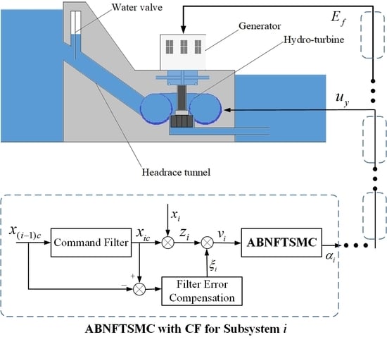Figure 4 shows a block diagram for the proposed ABNFTSMC with a CF for the design of a hydro-turbine governor in a HS. The stability of the nonlinear closed-loop system is verified by the multiple Lyapunov function stability theory. In addition, by combining the nonsingular fast terminal sliding mode control and CF techniques with the backstepping control procedure, the systems can both asymptotically achieve the desired trajectory within a finite time and avoid the problem of increasing complexity.

As shown in Figure 4, in the CF and error compensations to replace the virtual controls, the tracking error variables for the backstepping-based CF $z_i,i=1,\dots ,8$ are first defined as:

$$z_i={\tilde{x}}_i-x_{ic},\mathrm{for}i=1,\dots ,8$$

(15)

According to Notation 1, we know that ${\tilde{x}}_1=x_1$, ${\tilde{x}}_2=x_2$, ${\tilde{x}}_3=x_3$, ${\tilde{x}}_4=x_4$, ${\tilde{x}}_5=x_5$, ${\tilde{x}}_6=x_6$, ${\tilde{x}}_7=x_7$, and ${\tilde{x}}_8=x_8-E_{q_r}$. $x_{ic}$ is taken as the output of the finite-time CF that replaces the virtual controller ${\alpha }_{i-1}$ as the input.

Remark 4.

To eliminate the use of partial derivatives in the certain Lyapunov stability calculation for the virtual control signal$\alpha$in the conventional backstepping control procedure, the CF is utilized to approximate the virtual control$\alpha$such that the filtered output$x_{ic}$can then accurately track${\alpha }_{i-1}$. Moreover, we design the CF such that the tracking error$z_i$converges to zero in a finite time and eliminate the singularity problem in the conventional terminal sliding mode system. A nonsingular fast terminal sliding mode surface is selected as follows:

$$s_i=c_{i,1}{\dot{\tilde{x}}}_i+c_{i,2}{\tilde{x}}_i+c_{i,3}{\tilde{x}}_i^{p_i/q_i}$$

(16)

where$c_{i,1},c_{i,2},c_{i,3}$are positive constants and$p_i$and$q_i$are positive odd integers that satisfy$p_i>q_i$and$0<p_i/q_i<1$to avoid the intrinsic singularity problem. Once the sliding surface (16) converges to zero, i.e.,$s_i=0$, we have:

$${\dot{\tilde{x}}}_i=-\raisebox{1ex}{$1$}\!\left/ \!\raisebox{-1ex}{$c_{i,1}$}\right.\left(c_{i,2}{\tilde{x}}_i+c_{i,3}{\tilde{x}}_i^{p_i/q_i}\right)$$

(17)

which is the finite-time CF. Assuming that ${\dot{\tilde{x}}}_i={\dot{x}}_{ic}$, ${\tilde{x}}_i$ can be converted to $x_{ic}$ by filtering Equation (17) such that ${\tilde{x}}_i$ is the lead term for the sliding surface. In other words, $x_{ic}$ represents a point on the terminal sliding mode surface when ${\tilde{x}}_i$ reaches the mode. Therefore, a finite-time convergence and faster transient response can be guaranteed; moreover, the effects of internal disturbances, such as energy losses caused by a stochastic water flow, are eliminated to ensure robustness.

Remark 5.

It should be noted that the CF may cause filtering errors and may thus generate a small tracking error. To address the effect of the errors, the compensated signals will be defined.

Considering the filtering errors, the compensated tracking error signals$v_i$are obtained as

$$v_i=z_i-{\xi }_i,\mathrm{for}i=1,\dots ,8$$

(18)

and the error compensation signals${\xi }_i$can be derived as:

$$\begin{array}{l}{\dot{\xi }}_1=-k_1{\xi }_1+x_{2c}-{\alpha }_1+{\xi }_2,\\ {\dot{\xi }}_2=-k_2{\xi }_2+x_{3c}-{\alpha }_2+{\xi }_3,\\ {\dot{\xi }}_3=-k_3{\xi }_3+x_{4c}-{\alpha }_3+{\xi }_4,\\ {\dot{\xi }}_4=-k_4{\xi }_4+x_{5c}-{\alpha }_4+{\xi }_5,\\ {\dot{\xi }}_5=-k_5{\xi }_5-\raisebox{1ex}{$1$}\!\left/ \!\raisebox{-1ex}{$T_y$}\right.{\xi }_4,\\ {\dot{\xi }}_6=-k_6{\xi }_6+{\omega }_B(x_{7c}-{\alpha }_5+{\xi }_7),\\ {\dot{\xi }}_7=-k_7{\xi }_7-\raisebox{1ex}{$V_s\sin \delta $}\!\left/ \!\raisebox{-1ex}{$X_{d0}{T}_j$}\right.(x_{8c}-{\alpha }_6+{\xi }_8),\\ {\dot{\xi }}_8=-k_8{\xi }_8-\raisebox{1ex}{${\omega }_B$}\!\left/ \!\raisebox{-1ex}{$T_{d0}$}\right.{\xi }_7\end{array}$$

(19)

where${\xi }_i\left(0\right)=0,i=1,\dots ,8$, and$k_i\mathrm{for}i=1,\dots ,8$are positive constants. In addition,${\alpha }_j,j=1,\dots ,6$are virtual control inputs, which can be designed during the procedure of the finite-time CF backstepping control, as reported in (21). The error compensation in (19) both reduces the filtering errors such that the tracking error$z_i$converges to zero and ensures that the error compensation system is finite-time convergent. The proof regarding the error compensation signals (19) and the virtual control inputs (21) is derived in Section 4.

Remark 6.

The proposed sliding surface (16) combines the properties of the CF and nonsingular fast terminal sliding mode control such that the systems can ensure a rapid finite-time convergence without the singularity problem. By appropriately selecting the parameters$c_{i,1},c_{i,2},c_{i,3},p,q$, the system state attains an equilibrium in a finite time$t_{si}$, described as [29]:

$$t_{s_i}=c_{i,1}\left(\frac{p_i}{c_{i,2}\left(p_i-q_i\right)}\ln \frac{c_{i,2}{\tilde{x}}_i{\left(t_{r_i}\right)}^{\left(p_i-q_i\right)/p_i}+c_{i,3}}{c_{i,3}}\right)$$

(20)

where$t_{ri}$indicates the time to reach the terminal sliding surface$s_i$, which satisfies$t_{r_i}\le \left|s_i\left(t_0\right)\right|/{\eta }_i$, where$t_0$is the initial time; and${\eta }_i$is positive constants.

Remark 7.

In traditional backstepping control with CF scheme [30], the CF cannot determine the subsystem state to track the CF when tracking along the equilibrium point, which may cause the system state tracking time to increase. Therefore, the design of the nonsingular fast terminal sliding mode control combined with CF is adopted, which both accelerates the convergence and, through the design of the recursive relationship between the CF of each subsystem, resolves the singular problems caused by the nonsingular terminal sliding surface design when the differential process is analyzed.

$$\begin{array}{ll}{\alpha }_1& =-k_1{z}_1-\frac{1}{c_{1,1}}\left(c_{1,2}{x}_1+c_{1,3}{x}_1^{p_1/q_1}\right),\hfill \\ {\alpha }_2& =-k_2{z}_2-\frac{1}{c_{2,1}}\left(c_{2,2}{x}_2+c_{2,3}{x}_2^{p_2/q_2}\right),\hfill \\ {\alpha }_3& =\frac{{\pi }^2}{T_0{}^2}{x}_2-\frac{1}{Z_0{T}_0^3}\left(h_0-f_q^2-\frac{y_r^2}{x_5^2}{x}_4^2\right)-k_3{z}_3+x_4\hfill \\ & -\frac{1}{c_{3,1}}\left(c_{3,2}{x}_3+c_{3,3}{x}_3^{p_3/q_3}\right),\\ {\alpha }_4& =3{\pi }^2{x}_2-\frac{4}{Z_0{T}_0}\left(h_0-f_q^2{x}_4^2-\frac{y_r^2}{x_5{}^2}{x}_4^2\right)+{\tilde{x}}_5-k_4{z}_4\hfill \\ & -\frac{1}{c_{4,1}}\left(c_{4,2}{x}_4+c_{4,3}{x}_4^{p_4/q_4}\right),\\ {\alpha }_5& =\frac{1}{{\omega }_B}\left({\omega }_B-\frac{1}{c_{6,1}}\left(c_{6,2}{x}_6+c_{6,3}{x}_6^{p_6/q_6}\right)-k_6{z}_6\right),\hfill \\ {\alpha }_6& =-E_{qr}+\frac{X_{d0}}{V_s\sin \delta }(P_m-\frac{V_s^2\left(X_d{}_0-X_q\right)}{2X_{d0}{X}_q}\sin 2\delta -D_t\left(x_7-1\right)\hfill \\ & +\frac{T_j}{c_{7,1}}\left(c_{7,2}{x}_7+c_{7,3}{x}_7^{p_7/q_7}\right)+k_7{z}_7)\hfill \end{array}$$

(21)

Now, we are ready to present our primary results and demonstrate the above-described error compensation signals, virtual control inputs and system stability analysis.

Theorem 1.

Let us assume a HS model with energy losses and a terminal sliding mode surface described by Equations (14) and (16), respectively. If the finite-time CF is chosen as in Equation (17), the error compensation signals and virtual signals are respectively determined as given in Equations (19) and (21). The control laws, i.e., the TGC$u_y$for the hydro-turbine and the voltage controller$E_f$for the generator, are respectively given by:

$$u_y= \left(x_5-y_0-{\xi }_4\right)-\frac{T_y}{c_{5,1}}\left(c_{5,2}{x}_5+c_{5,3}{x}_5^{p_5/q_5}\right)-T_y{k}_5{z}_5$$

(22)

$$E_f=\frac{X_d{x}_8}{X_{d0}}-\frac{X_d-X_{d0}}{X_{d0}}{V}_s\cos \delta -\frac{T_{d0}}{c_{8,1}{\omega }_B}\left(c_{8,2}{\tilde{x}}_8+c_{8,3}{\tilde{x}}_8^{p_8/q_8}\right)-{\xi }_7-\frac{T_{d0}}{{\omega }_B}{k}_8{z}_8$$

(23)

In addition, the finite time can be obtained as follows:

$$t_s\le {\displaystyle \sum _{n=1}^8{c}_{n,1}\left(\frac{p_n}{c_{n,2}\left(p_n-q_n\right)}\ln \frac{c_{n,2}{x}_n{\left(t_{r_n}\right)}^{\left(p_n-q_n\right)/p_n}+c_{n,3}}{c_{n,3}}\right)}$$

(24)

Therefore, both the tracking error ${\tilde{x}}_i$ and its derivative ${\dot{\tilde{x}}}_i$ will converge to zero in a finite time such that all subsystem states can rapidly track the rated reference value in finite time guaranteed global asymptotic stability.

Proof of Theorem 1.

The excepted result can be formulated by the following steps. □

3.1. Step 1 (Subsystem 1)

First, a positive definite Lyapunov function for Subsystem 1, i.e., the relative value of the water flow for the PS, is defined as:

$$V_1=\raisebox{1ex}{$1$}\!\left/ \!\raisebox{-1ex}{$2$}\right.v_1^2$$

(25)

The derivative of $V_1$ is:

$${\dot{V}}_1=v_1\left({\dot{z}}_1-{\dot{\xi }}_1\right)$$

(26)

From the error compensation signal (19) and the CF (17), Equation (26) can be rewritten as:

$${\dot{V}}_1=v_1\left({\tilde{x}}_2+\frac{1}{c_{1,1}}\left(c_{1,2}{\tilde{x}}_1+c_{1,3}{\tilde{x}}_1^{p_1/q_1}\right)+k_1{\xi }_1-\left(x_{2c}-{\alpha }_1\right)-{\xi }_2\right)$$

(27)

From Equation (27), it can be easily demonstrated that the virtual control ${\alpha }_1$ can be chosen by (21). Thus, it is straightforward to show that Equation (27) can be further expressed as:

$${\dot{V}}_1=-k_1{v}_1^2+v_1{v}_2$$

(28)

when $v_2=0$, ${\dot{V}}_1<0$, Consequently, the state $x_1$, i.e., Subsystem 1, will be asymptotically stable. Moreover, according to Remark 6, the finite time $t_1$ can be obtained as follows.

$$t_1\le c_{1,1}\left(\frac{p_1}{c_{1,2}\left(p_1-q_1\right)}\ln \frac{c_{1,2}{x}_1{\left(t_{r_1}\right)}^{\left(p_1-q_1\right)/p_1}+c_{1,3}}{c_{1,3}}\right)$$

(29)

3.2. Step 2 (Subsystem 2)

We select the Lyapunov function for Subsystem 2, i.e., the relative velocity of the water flow for the PS, as follows:

$$V_2=V_1+\raisebox{1ex}{$1$}\!\left/ \!\raisebox{-1ex}{$2$}\right.v_2^2$$

(30)

Taking the derivative of $V_2$ yields:

$${\dot{V}}_2={\dot{V}}_1+v_2\left({\dot{z}}_2-{\dot{\xi }}_2\right)$$

(31)

Considering the CF (17) and the derivation of the error compensation signal (19), we have:

$${\dot{V}}_2={\dot{V}}_1+v_2\left(v_3+{\alpha }_2+\frac{1}{c_{2,1}}\left(c_{2,2}{\tilde{x}}_2+c_{2,3}{\tilde{x}}_2^{p_2/q_2}\right)+k_2{\xi }_2\right)$$

(32)

Based on Equation (32), the virtual control ${\alpha }_2$ can be derived from Equation (21). Therefore, Equation (32) can be rewritten as:

$$\begin{array}{ll}{\dot{V}}_2& ={\dot{V}}_1-k_2{v}_2^2+v_2{v}_3\\ & =-k_1{v}_1^2-k_2{v}_2^2+v_2{v}_3\end{array}$$

(33)

From Equation (33), ${\dot{V}}_2<0$ when $v_3=0$, and the states $x_1$ and $x_2$ will be asymptotically stable. In addition, the finite time $t_2$ for Subsystem 2 can be derived as follows:

$$t_2\le c_{2,1}\left(\frac{p_2}{c_{2,2}\left(p_2-q_2\right)}\ln \frac{c_{2,2}{x}_2{\left(t_{r_2}\right)}^{\left(p_2-q_2\right)/p_2}+c_{2,3}}{c_{2,3}}\right)$$

(34)

3.3. Step 3 (Subsystem 3)

We consider the following Lyapunov function:

$$V_4=V_3+\raisebox{1ex}{$1$}\!\left/ \!\raisebox{-1ex}{$2$}\right.v_4^2$$

(35)

Differentiating $V_3$ with respect to time, we have:

$${\dot{V}}_3={\dot{V}}_2+v_3\left({\dot{z}}_3-{\dot{\xi }}_3\right)$$

(36)

Substituting the CF (17) and the derivation of the error compensation signal (19) into Equation (36) yields:

$${\dot{V}}_3={\dot{V}}_2+v_3(-\frac{{\pi }^2}{T_0{}^2}{\tilde{x}}_2+\frac{1}{Z_0{T}_0^3}\left(h_0-f_q^2{\tilde{x}}_4^2-\frac{y_r^2}{x_5^2}{\tilde{x}}_4^2\right)+k_3{\xi }_3+{\alpha }_3+v_4-{\tilde{x}}_4+\frac{1}{c_{3,1}}\left(c_{3,2}{\tilde{x}}_3+c_{3,3}{\tilde{x}}_3^{p_3/q_3}\right))$$

(37)

From Equation (37), it can be proven that the virtual control ${\alpha }_3$ can be determined by Equation (21). Thus, Equation (37) can be rewritten as:

$$\begin{array}{ll}{\dot{V}}_3& ={\dot{V}}_2-k_3{v}_3^2+v_3{v}_4\\ & =-k_1{v}_1^2-k_2{v}_2^2-k_3{v}_3^2+v_3{v}_4\end{array}$$

(38)

Obviously, the states $x_1$, $x_2$ and $x_3$ will be asymptotically stable when ${\dot{V}}_3<0$ under v₄ = 0. In addition, the finite time $t_3$ for Subsystem 3 can be defined as follows:

$$t_3\le c_{3,1}\left(\frac{p_3}{c_{3,2}\left(p_3-q_3\right)}\ln \frac{c_{3,2}{x}_3{\left(t_{r_3}\right)}^{\left(p_3-q_3\right)/p_3}+c_{3,3}}{c_{3,3}}\right)$$

(39)

3.4. Step 4 (Subsystem 4)

We select the Lyapunov function for Subsystem 4:

$$V_4=V_3+\raisebox{1ex}{$1$}\!\left/ \!\raisebox{-1ex}{$2$}\right.v_4^2$$

(40)

Then, it follows that:

$${\dot{V}}_4={\dot{V}}_3+v_4\left({\dot{z}}_4-{\dot{\xi }}_4\right)$$

(41)

According to Equations (14), (17), and (19), Equation (41) can be obtained:

$${\dot{V}}_4={\dot{V}}_3+v_4(-3{\pi }^2{\tilde{x}}_2+\frac{4}{Z_0{T}_0}\left(h_0-f_q^2{\tilde{x}}_4^2-\frac{y_r^2}{x_5{}^2}{\tilde{x}}_4^2\right)+k_4{\xi }_4+v_5-{\tilde{x}}_5+{\alpha }_4+\frac{1}{c_{4,1}}\left(c_{4,2}{\tilde{x}}_4+c_{4,3}{\tilde{x}}_4^{p_4/q_4}\right))$$

(42)

Hence, the virtual control ${\alpha }_4$ can be defined from Equation (21). Then, we obtain:

$$\begin{array}{ll}{\dot{V}}_4& ={\dot{V}}_3-k_4{v}_4^2+v_4{v}_5\\ & =-k_1{v}_1^2-k_2{v}_2^2-k_3{v}_3^2-k_4{v}_4^2+v_4{v}_5\end{array}$$

(43)

when $v_5=0$, ${\dot{V}}_4<0$, the states $x_1$ to $x_4$ will be asymptotically stable. The finite time $t_4$ for Subsystem 4 is:

$$t_4\le c_{4,1}\left(\frac{p_4}{c_{4,2}\left(p_4-q_4\right)}\ln \frac{c_{4,2}{x}_4{\left(t_{r_4}\right)}^{\left(p_4-q_4\right)/p_4}+c_{43}}{c_{43}}\right)$$

(44)

3.5. Step 5 (Subsystem 5)

We choose the Lyapunov function for Subsystem 5:

$$V_5=V_4+\raisebox{1ex}{$1$}\!\left/ \!\raisebox{-1ex}{$2$}\right.v_5^2$$

(45)

Therefore, the derivative of $V_5$ is:

$${\dot{V}}_5={\dot{V}}_4+v_5\left({\dot{z}}_5-{\dot{\xi }}_5\right)$$

(46)

Considering Equations (14), (17), and (19), Equation (46) can be rewritten as:

$${\dot{V}}_5={\dot{V}}_4+v_5\left(\frac{1}{T_y}\left(u_y-x_5+y_0+{\xi }_4\right)+k_5{\xi }_5\right)+v_5\left(\frac{1}{c_{5,1}}\left(c_{5,2}{\tilde{x}}_5+c_{5,3}{\tilde{x}}_5^{p_5/q_5}\right)\right)$$

(47)

According to the virtual control ${\alpha }_2$ from Equations (21) and (47) can be expressed as:

$$\begin{array}{ll}{\dot{V}}_5& ={\dot{V}}_4-k_5{v}_5^2\\ & =-k_1{v}_1^2-k_2{v}_2^2-k_3{v}_3^2-k_4{v}_4^2-k_5{v}_5^2\end{array}$$

(48)

In addition, for the result in which ${\dot{V}}_5<0$ can easily show that the states $x_1$ to $x_5$ will be asymptotically stable. In other words, the hydro-turbine governor unit can achieve global asymptotic stability under a backstepping TGC (22). Additionally, the finite time of Subsystem 5 can be described as:

$$t_5\le c_{5,1}\left(\frac{p_5}{c_{5,2}\left(p_5-q_5\right)}\ln \frac{c_{5,2}{x}_5{\left(t_{r_5}\right)}^{\left(p_5-q_5\right)/p_5}+c_{5,3}}{c_{5,3}}\right)$$

(49)

3.6. Step 6 (Subsystem 6)

Next, we discuss Subsystem 6 to 8, which represent the three states of the generator control unit. First, the Lyapunov function $V_6$ for Subsystem 4 can be defined as:

$$V_6=V_5+\raisebox{1ex}{$1$}\!\left/ \!\raisebox{-1ex}{$2$}\right.v_6^2$$

(50)

Then, the derivative of $V_6$ is:

$${\dot{V}}_6={\dot{V}}_5+v_6\left({\dot{z}}_6-{\dot{\xi }}_6\right)$$

(51)

Combining the CF (17) and error compensation signal (19) into Equation (51), yield:

$${\dot{V}}_6={\dot{V}}_5+v_6({\omega }_B\left({\tilde{x}}_7-1\right)+\frac{1}{c_{6,1}}\left(c_{6,2}{\tilde{x}}_6+c_{6,3}{\tilde{x}}_6^{p_6/q_6}\right)+k_6{\xi }_6-{\omega }_B\left(x_{7c}-{\alpha }_5+{\xi }_7\right))$$

(52)

Therefore, it can be proved that the virtual control ${\alpha }_5$ can be determined by (21). Thus, the Equation (52) can be rewritten as:

$$\begin{array}{ll}{\dot{V}}_6& ={\dot{V}}_5-k_6{v}_6^2+{\omega }_B{v}_6{v}_7\\ & =-k_1{v}_1^2-k_2{v}_2^2-k_3{v}_3^2-k_4{v}_4^2-k_5{v}_5^2-k_6{v}_6^2+{\omega }_B{v}_6{v}_7\end{array}$$

(53)

when v₇ = 0, ${\dot{V}}_6<0$, it means that Subsystem 6 will be asymptotically stable, and the finite time can be defined as:

$$t_6\le c_{6,1}\left(\frac{p_6}{c_{6,2}\left(p_6-q_6\right)}\ln \frac{c_{6,2}{x}_6{\left(t_{r_6}\right)}^{\left(p_6-q_6\right)/p_6}+c_{6,3}}{c_{6,3}}\right)$$

(54)

3.7. Step 7 (Subsystem 7)

We consider the following Lyapunov function:

$$V_7=V_6+\raisebox{1ex}{$1$}\!\left/ \!\raisebox{-1ex}{$2$}\right.v_7^2$$

(55)

Taking the derivative of $V_7$ yields:

$${\dot{V}}_7={\dot{V}}_6+v_7\left({\dot{z}}_7-{\dot{\xi }}_7\right)$$

(56)

then, the CF (17) and the error compensation signal (19) are combined into Equation (56), we have:

$$\begin{array}{cc}{\dot{V}}_7& ={\dot{V}}_6+v_7(\frac{1}{T_j}(P_m-\frac{{\tilde{x}}_8{V}_s\sin \delta }{X_{d0}}-D_t\left({\tilde{x}}_7-1\right)-\frac{V_s^2\left(X_d{}_0-X_q\right)}{2X_{d0}{X}_q}\sin 2\delta )+\frac{1}{c_{7,1}}\left(c_{7,2}{\tilde{x}}_7+c_{7,3}{\tilde{x}}_7^{p_7/q_7}\right)\\ & +k_7{\xi }_7+\frac{V_s\sin \delta }{X_{d0}{T}_j}(x_{8c}-{\alpha }_6+E_{qr}-E_{qr}+{\xi }_8))\hfill \end{array}$$

(57)

Thus, it can be seen that the virtual control ${\alpha }_6$ can be derived from (21). Equation (57) can then be rewritten as:

$${\dot{V}}_7={\dot{V}}_6-k_7{v}_7^2-\frac{V_s\sin \delta }{T_j{X}_{d0}}{v}_7{v}_8$$

(58)

It is obvious that Subsystem 6 will be asymptotically stable when ${\dot{V}}_7<0$ under $v_8=0$, and the finite time can obtained as:

$$t_7\le c_{7,1}\left(\frac{p_7}{c_{7,2}\left(p_7-q_7\right)}\ln \frac{c_{7,2}{x}_7{\left(t_{r_7}\right)}^{\left(p_7-q_7\right)/p_7}+c_{7,3}}{c_{7,3}}\right)$$

(59)

3.8. Step 8 (Subsystem 8)

Finally, the Lyapunov function for Subsystem 8, i.e., internal transient voltage for generator, can be chosen:

$$V_8=V_7+\raisebox{1ex}{$1$}\!\left/ \!\raisebox{-1ex}{$2$}\right.v_8^2$$

(60)

Then, the derivative of $V_8$ is:

$${\dot{V}}_8={\dot{V}}_7+v_8\left({\dot{z}}_8-{\dot{\xi }}_8\right)$$

(61)

According to the (14), (17) and (19), Equation (61) can be obtained:

$${\dot{V}}_8={\dot{V}}_7+v_8(-\frac{{\omega }_B}{T_{d0}}\frac{X_d}{X_{d0}}{x}_8+\frac{{\omega }_B}{T_{d0}}\frac{X_d-X_{d0}}{X_{d0}}{V}_s\cos \delta +\frac{{\omega }_B{E}_f}{T_{d0}}+\frac{1}{c_{8,1}}\left(c_{8,2}{\tilde{x}}_8+c_{8,3}{\tilde{x}}_8^{p_8/q_8}\right)+k_8{\xi }_8+\frac{{\omega }_B{\xi }_7}{T_{d0}})$$

(62)

From Equation (62), it is straightforward to verify that the backstepping voltage controller $E_f$ for generator satisfies assumption of Theorem 1. Therefore, Equation (62) can be rewritten as:

$${\dot{V}}_8={\dot{V}}_7-k_8{v}_8^2$$

(63)

This shows the HS (14) will be asymptotically stable under the control (23) when ${\dot{V}}_8<0$. Since the asymptotic stability implies its compensation tracking error signals $v_i,\mathrm{for}i=1,\dots ,8$ will converge to zero in a finite time. Therefore, the HS (14) can approach the desired trajectory by the proposed control strategy for governor guide vane and voltage of generator. Otherwise, the finite time of Subsystem 8 can be described as:

$$t_8\le c_{8,1}\left(\frac{p_8}{c_{8,2}\left(p_8-q_8\right)}\ln \frac{c_{8,2}{x}_8{\left(t_{r_8}\right)}^{\left(p_8-q_8\right)/p_8}+c_{8,3}}{c_{8,3}}\right)$$

(64)

Finally, from Equations (29), (34), (39), (44), (49), (54), (59) and (64), it can easily be demonstrated that the finite time $t_s$ for the entire HS can be expressed by Equation (24). Thus, the proof is complete.

4. Simulation Results

The objective of this section is to evaluate the performance of the proposed ABNFTSMC scheme with CF for the Nazi Gorge HS in China. Firstly, we employ the ABNFTSMC with CF in two stochastic water flow intensity cases for the HS. For each situation, the designed ABNFTSMC schemes are simulated and compared with the ABSMC method [15] in MATLAB software. The ABNFTSMC strategy is regarded as successful if its implementation in a HS can improve both the transient stability and energy conversion efficiency while also meeting the critical requirements. Taking the Nazi Gorge HS as an example, the detailed parameters are given in [25]. The density of water $\gamma =9.81(\mathrm{kN}/{\mathrm{m}}^3)$, and the coefficient of volume loss $k_v=0.0025$. According to IEC 60,308 [31] and IEC 61,362 [32], the initial values are defined as q₀ = 30.86 (m³/s), y₀ = 161.95 (mm), δ₀ = 36.62 (rad), ω₀ = 409.17 (rad/s), and $E_{q_0}$ = 6294 (kW). In addition, the rated reference values are expressed as q_r = 32.86 (m³/s), y_r = 205 (mm), δr = 44.86 (rad), ω_r = 428.6 (rad/s) and $E_{q_r}$ = 6300 (kW).

• Stochastic Water Flow Model

To compare the proposed control scheme with the ABSMC method [15], a stochastic water flow was considered. The constantly changing water flow in a hydro-turbine has been considered as a stochastic perturbation for the HS. Based on [25,33], the water flow model considering two stochastic intensities of water flow, $D=0.01$ and $D=0.6$, is shown in Figure 5.

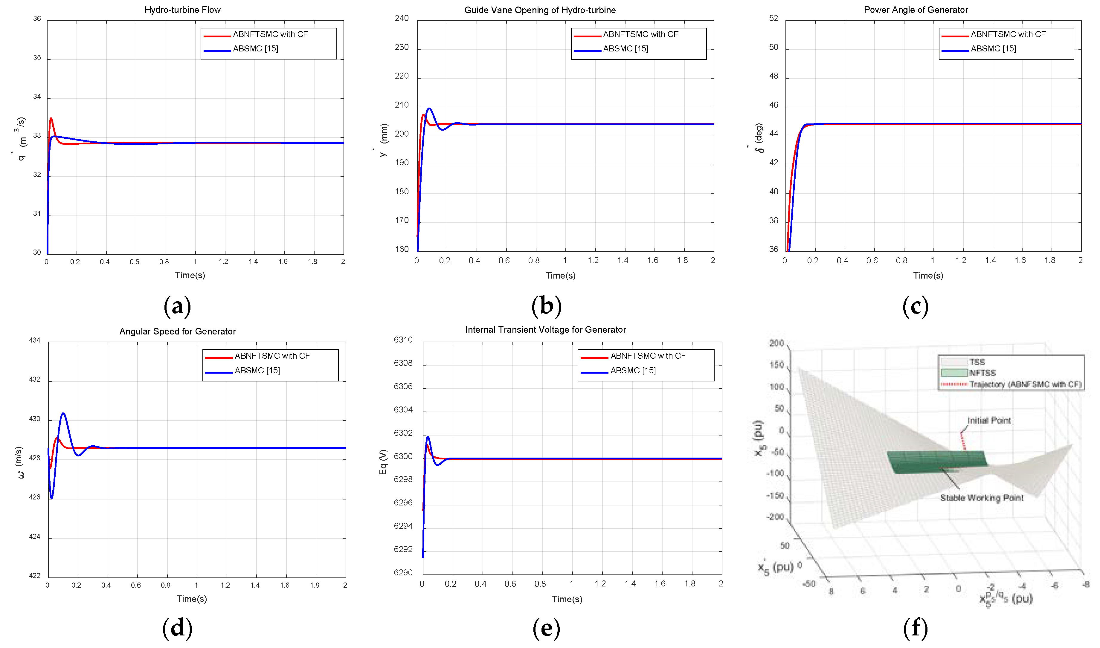
4.1. Case 1. Stochastic intensity of the water flow ($D=0.01$)

Figure 6a–e present a comparison of the tracking trajectories of system state variables $q^{\ast }$, $y^{\ast }$, ${\delta }^{\ast }$, ω*, $E_q$ for the proposed ABNFTSMC with the CF scheme (red line) and the traditional ABSMC method [15] (blue line), respectively.

From Figure 6, it is obvious that the realistic values for $q^{*}$, $y^{*}$, ${\delta }^{*}$, ${\omega }^{*}$, $E_q$ gradually tend to the rated reference values for $q_r$, $y_r$, ${\delta }_r$, ${\omega }_r$, $E_{qr}$, indicating that the relative value of the hydro-turbine flow $(q)$, the relative deviation of the GV opening $(y)$ for the hydro-turbine, the rotor angle relative deviation $(\delta )$ for the generator, the angular speed relative deviation $(\omega )$ for the generator, and the internal transient voltage $(E_q)$ for the generator can rapidly track the desired reference signals. It is clearly demonstrated that each closed-loop subsystem has a superior performance, with faster high-precision tracking within a finite time and no singularity; meanwhile, the system has a smaller overshoot of the transient response than the traditional ABSMC method [15].

Figure 6f shows a three-dimensional phase trajectory curve of Subsystem 5 for a nonsingular fast terminal sliding surface (NFTSS) and terminal sliding surface (TSS) scheme. The green area is the proposed TSS without a singularity, the gray area is the TSS containing a singularity, and the red line is the tracking trajectory for Subsystem 5. Hence, we conclude that from any initial state, the system state can rapidly converge to the origin, i.e., stability can be achieved from any point along the nonsingular TSS in finite time without any singularities.

Table 1. The comparison of power losses under stochastic intensity $D=0.01$.

Energy Loss	ABNFTSMC with CF	ABSMC [15]
$P_{wz}$	2.52 (kW)	2.98 (kW)
$P_{ww1}$	478.8 (kW)	566 (kW)
$P_{ww2}$	1565.4 (kW)	1877.4 (kW)
$P_{wj}$	22.68 (kW)	26.82 (kW)
$P_v$	90.072 (kW)	107.28 (kW)
$P_p$	35.28 (kW)	41.72 (kW)
$P_m$	327.6 (kW)	357.6 (kW)
$P_{\Sigma }$	2522.352 (kW)	2979.8 (kW)

shows the energy losses with stochastic intensity $D=0.01$ for comparison between our proposed control scheme and ABSMC [15].

As shown in Table 1, the primary contributions of the energy losses come from the impact loss for the spiral case $(P_{ww2})$. It is clear that our proposed control scheme can reduce the power loss by 312 kW compared with the impact loss for the spiral case with ABSMC [15]. Moreover, the overall energy losses $P_{\Sigma }$ under a stochastic intensity of $D=0.01$ for our proposed ABNFTSMC with CF can reduce the loss by 457.448 kW compared with that of the ABSMC [15].

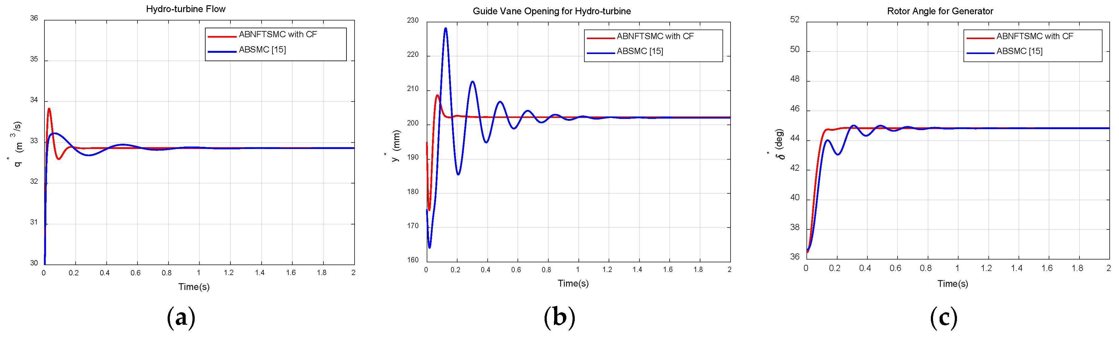
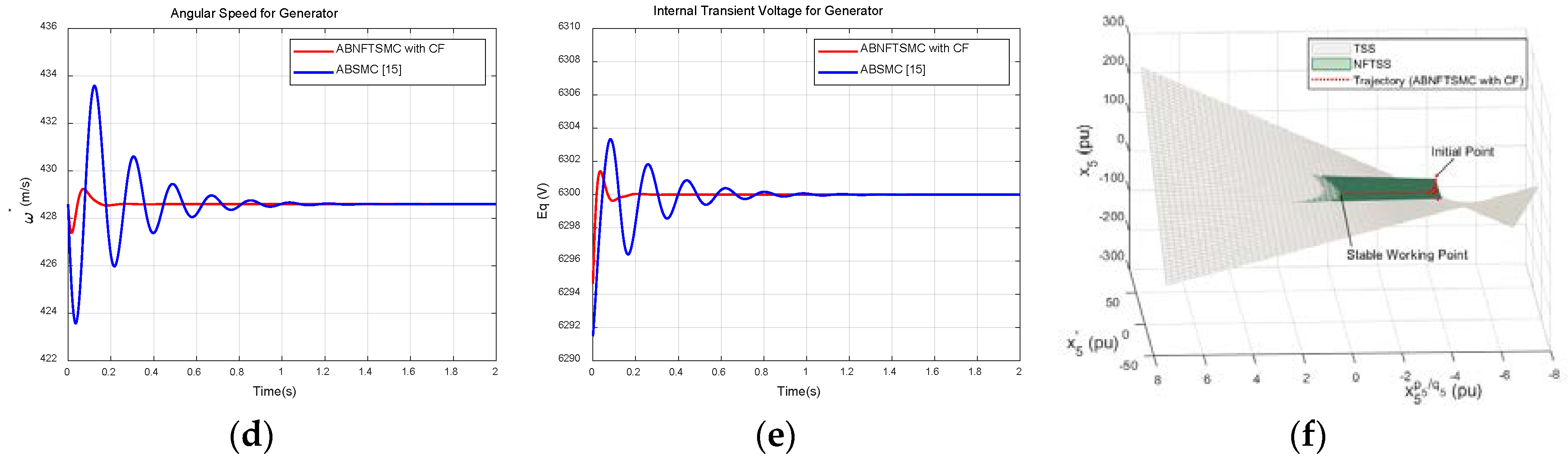
4.2. Case 2. Stochastic intensity of the water flow ($D=0.6$)

We simulated a case in which the stochastic intensity of the water flow was 0.6. Compared with the results for a stochastic intensity of 0.01, a greater chattering effect is produced by the energy losses from internal disturbances. Although the overall system state variables of the method in [15] and those of the proposed ABNFTSMC with CF both track the rated reference value, the proposed control scheme produces a better transient response. The responses of the two methods are demonstrated in Figure 7a–e. We can observe that for these control strategies, all system state variables track the desired reference signals in a timely manner. However, the ABSMC scheme exhibited a larger chatter effect and a poor convergence time due to its operating condition, i.e., the controller limit and nonsingularity problem.

Similarly, a three-dimensional phase trajectory curve of Subsystem 5 for a NFTSS and TSS is shown in Figure 7f. It is straightforward to show that from any initial state, the system states can progress along the NFTSS (green plant) to achieve a stable working point in a finite time, which effectively shows that the system states avoid passing through singular points (gray area).

Table 2. The comparison of power losses under stochastic intensity $D=0.6$.

Energy Loss	ABNFTSMC with CF	ABSMC [15]
$P_{wz}$	3.54 (kW)	4.14 (kW)
$P_{ww1}$	672.6 (kW)	786.6 (kW)
$P_{ww2}$	2265.6 (kW)	2691 (kW)
$P_{wj}$	31.86 (kW)	37.26 (kW)
$P_v$	130.98 (kW)	153.18 (kW)
$P_p$	46.02 (kW)	53.82 (kW)
$P_m$	389.4 (kW)	414 (kW)
$P_{\Sigma }$	3540 (kW)	4140 (kW)

shows the energy losses for a stochastic intensity of $D=0.6$, for a comparison between our proposed control scheme and the ABSMC [15]. It can be seen that the primary contributions of the energy losses come from the impact loss of the spiral case $(P_{ww2})$, and the proposed control scheme can efficiently reduce approximately 425.4 kW for the power loss compared with the ABSMC [15]. In addition, the overall energy losses $P_{\Sigma }$ under a stochastic intensity of $D=0.6$ for our proposed ABNFTSMC with CF are effectively reduced by 600 kW compared with the ABSMC [15].

From Figure 8, it can be clearly seen that the proposed control method is superior to the ABSMC method [15] in the adjustment of the mechanical power of the hydro-turbine and the electrical power of the generator. The conversion efficiency of the HS shows that the energy loss increases with increasing stochastic intensity, along with the electrical power of the HS. As shown in

Table 3. The comparison of power conversion efficiency.

Mechanical Power and Conversion Efficiency of Hydro-Turbine
	SI	D = 0.6	D = 0.01
Control Scheme
MP (ABNFTSMC with CF)		32,636 (kW)	31,500 (kW)
MP (ABSMC) [15]		32,260 (kW)	31,137 (kW)
CEt (ABNFTSMC with CF)		96.86%	95%
CEt (ABSMC) [15]		95.8%	93.96%
Electrical Power and Conversion Efficiency of Generator
EP (ABNFTSMC with CF)		31,510 (kW)	29,730 (kW)
EP (ABSMC) [15]		30,770 (kW)	29,020 (kW)
CEg (ABNFTSMC with CF)		96.55%	94.38%
CEg (ABSMC) [15]		95.38%	93.24%

, for the conversion efficiency of mechanical power, the proposed method with a stochastic intensity of 0.6 reaches an efficiency of 96.86%; however, the ABSMC [15] reaches an efficiency of only 95.8%. Moreover, for the conversion efficiency of electrical power, the proposed approach can achieve 96.55%; in contrast, the ABSMC [15] achieves only 95.38%.

From Figure 8 and Table 3, it can be clearly seen that the proposed control method is superior to the ABSMC method [15] in adjusting the mechanical power of the hydro-turbine and the electrical power of the generator.

The conversion efficiency results of the HS demonstrate that the energy losses increase with increasing stochastic intensity and electrical power of the HS. In Table 3, for the conversion efficiency of mechanical power, the proposed method with a stochastic intensity of 0.6 can reach 96.86%; however, the ABSMC [15] method reaches only 95.8%. Moreover, for the conversion efficiency of electrical power, the proposed approach can achieve 96.55%, whereas the ABSMC [15] reaches only 95.38%. In addition, the total mechanical power (MP) of the hydro-turbine for the proposed control scheme with a flow water stochastic intensity of 0.01 and 0.6 is increased by 363 and 376 kW compared with the ABSMC [15] method. In addition, the total electrical power of the generator for the proposed control scheme with a water flow stochastic intensity of 0.01 and 0.6 is increased by 710 and 740 kW compared with the ABSMC method [15]. Hence, it has been demonstrated the proposed control scheme can effectively improve the generation efficiency and stability of a hydropower plant.

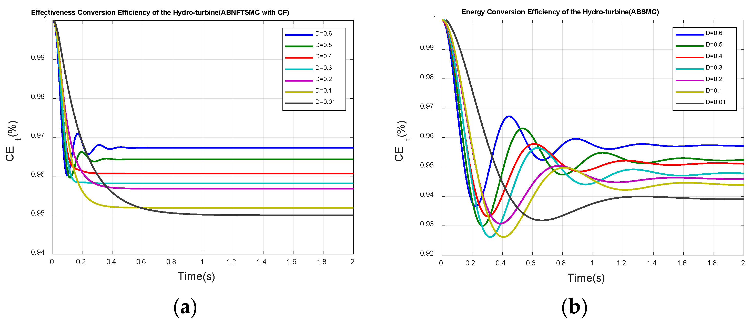
The conversion efficiency of the hydro-turbine and generator for our proposed control method and the ABSMC method [15] based on different stochastic intensities is shown in Figure 9 and Figure 10, respectively. It is clear that the proposed control scheme has a higher energy conversion efficiency as well as a superior transient response and stability, thus adding to the overall reliability and efficiency of power generation.

5. Conclusions

In this paper, an eight-order nonlinear HS with a stochastic water flow is considered for a real-world complete large-scale HS model. Consequently, an adaptive backstepping control strategy combined with nonsingular fast terminal sliding mode control is utilized for such a HS to address the internal energy losses, including hydraulic and electrical losses. By employing a nonsingular fast terminal SMC, the HS can satisfy a finite-time convergence without a singularity problem and can achieve a rapid transient response, and high precision tracking. Moreover, the CF backstepping approach can provide an approximation of the derivative of the virtual control to suppress the internal disturbances of the HS caused by the stochastic water flow. To evaluate the performance of the proposed scheme, the water flow model was considered for two stochastic intensities, 0.01 and 0.6; the results indicate that an increased water flow stochastic intensity will lead to an increased internal energy loss, influencing the MP, and electrical power generation. According to the simulation results, compared with the ABSMC method in [15], the system states for the ABNFTSMC method can converge rapidly to the origin in a finite time without any singularities. In terms of the energy and power loss, the proposed ABNFTSMC also provides an improvement in both stochastic water flow cases. Furthermore, for the proposed ABNFTSMC, the mechanical power of the hydro-turbine, the electrical power of the generator, and the conversion efficiency outperform when compared with the ABSMC method. Therefore, it is firmly to conclude that the ABNFTSMC strategy achieves superior performance for a large-scale HS. Finally, we believe that our approach holds great promise for solving a variety of practical problems and challenges.