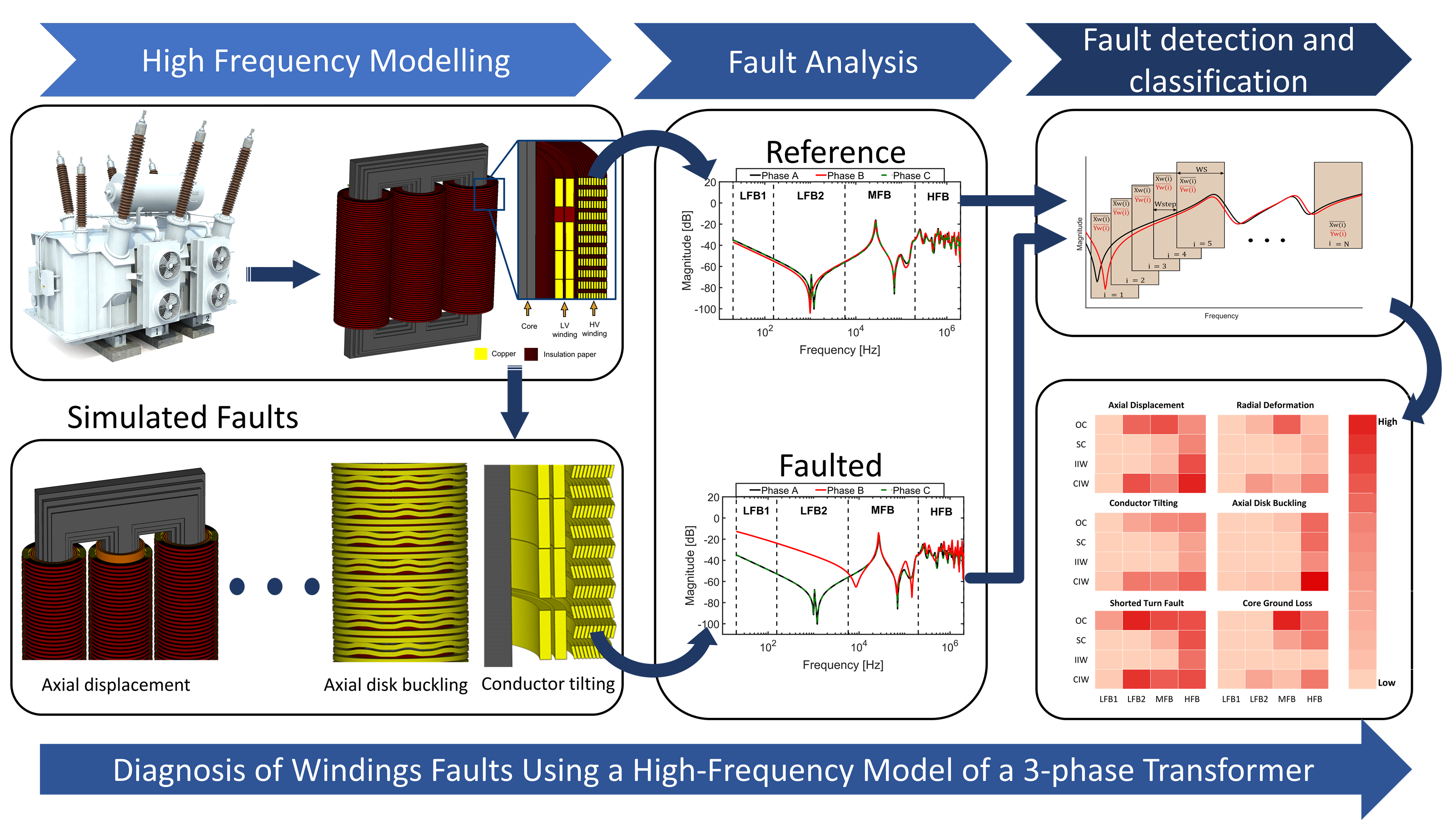
A Comprehensive Analysis of Windings Electrical and Mechanical Faults Using a High-Frequency Model

Abstract

The measurement procedures for frequency response analysis (FRA) of power transformers are well documented in IEC and IEEE standards. However, the interpretation of FRA results is still far from reaching an accepted methodology and is limited to the analysis of the experts. The dilemma is that there are limited case studies available to understand the effect of different faults. Additionally, due to the destructive nature, it is not possible to apply the real mechanical deformations in the transformer windings to obtain the data. To solve these issues, in this contribution, the physical geometry of a three-phase transformer is simulated using 3D finite integration analysis to emulate the real transformer operation. The novelty of this model is that FRA traces are directly obtained from the 3D model of windings without estimating and solving lumped parameter circuit models. At first, the method is validated with a simple experimental setup. Afterwards, different mechanical and electrical faults are simulated, and their effects on FRA are discussed objectively. A key contribution of this paper is the winding assessment factor it introduces based on the standard deviation of difference (SDD) to detect and classify different electrical and mechanical faults. The results reveal that the proposed model provides the ability of precise and accurate fault simulation. By using SDD, different deviation patterns can be characterized for different faults, which makes fault classification possible. Thus, it provides a way forward towards the establishment of the standard algorithm for a reliable and automatic assessment of transformer FRA results.

1. Introduction

Power transformers are considered as one of the most expensive assets and the vital links in electrical power transmission and distribution networks. Due to the rapid growth of the power grid, long-term exposure of the transformers to the system faults and significant ageing of the transformer fleet worldwide has increased the likelihood of internal transformer failures and/or catastrophic failures. Most of the transformers currently in operation were installed during the period of rapid economic growth, prior to the 1980s. It means that the majority of the transformer fleet is approaching or already has passed its expected lifespan [1]. Moreover, in the future, the number of ageing transformers is expected to increase further. This poses a significant risk to the system reliability and service continuity for the power utilities as transformer failures can cause considerable and unforeseeable costs, power outages, and environmental hazards due to oil spillage. Consequently, condition assessment and diagnostic techniques are essential to improve network reliability. Therefore, different diagnostic methods have been established to detect faults within power transformers. The dissolved gas analysis (DGA), partial discharge (PD) measurement, thermal analysis (TA), and transformer function (TF) assessment are the main diagnostic methods introduced in the literature [2,3].

Nowadays, winding deformation is one of the major reasons behind transformer failures. Winding deformations may result from very large electromagnetic forces generated when high short circuit current flows into the windings [4]. Among these winding deformations, radial deformation (Compression and Hoop-tension failure), axial winding elongation—“Telescoping”, bulk and localized movement of windings are the frequent mechanical faults. Though the minor winding deformations do not necessarily lead to an immediate transformer failure, however, its mechanical integrity is greatly reduced to withstand future mechanical and electrical stresses. Therefore, the detection of minor winding deformations is very essential to take immediate remedial actions [5,6].

Frequency response analysis (FRA) is a powerful, non-destructive, and non-intrusive method to detect various mechanical and electrical faults within power transformers without internal inspection [7]. Recent studies in the field of FRA have led to the standardization of its measurement procedures as described in IEEE and IEC standards [8,9]. However, the interpretation of FRA results is still far from reaching an accepted and definite methodology and is limited to the analysis of the experts in the field. Hence, a systematic approach for the interpretation of FRA results is of essential need. Currently, there is a CIGRE working group A2.53, aiming to produce a technical brochure containing guidelines for interpretation of FRA [10].

In the literature, mainly circuit models (black box, white box, grey box, etc.) are employed for interpretation of FRA results [11,12,13]. In these circuit models, different sections of transformer windings are represented by circuit elements, such as resistors, inductors, and capacitors, in which the values are extracted either by analytical equations or through finite element methods (FEM). Afterwards, the values of these parameters are altered to model and study the impact of various mechanical defects on FRA traces. However, these circuit models have some drawbacks, such as they require an accurate estimation of the winding parameters to model and study the impact of different faults on FRA traces. Secondly, their response is limited to a certain frequency (up to 500 kHz) due to difficulty in solving turn-based parameters. Thirdly, some mechanical changes are difficult to model, and the conversion process involves extra uncertainty. In addition, constant values of the parameters are employed while these parameters are frequency dependent. Lastly, in all the circuit model studies, the values of one or two parameters are changed to investigate the impact of various mechanical faults, while mechanical deformations like radial deformation, telescoping, and conductor tilting are much more complicated and involve the contribution of more than one parameter [6]. While to detect the minor winding deformations, precise and accurate fault simulation is essential. Furthermore, not much attention was given to the impact of incipient faults on different connection schemes, especially short-circuit and inter-winding connection schemes, which proved to possess high sensitivity against winding deformation faults [6].

In contrast to the circuit models, in this contribution, the physical geometry of a three-phase transformer is simulated using 3D finite integration analysis to emulate the real transformer and FRA measurement operations. The novelty of this model is that FRA traces are directly obtained from the 3D high-frequency model (HF-model) of windings without estimating and solving lumped parameter circuit models. At first, the method is validated with a simple experimental setup for both healthy and deformed windings. Afterwards, comprehensive simulated fault analyses are conducted on a three-phase transformer model. For this purpose, different electrical and mechanical faults are simulated on low voltage (LV) and high voltage (HV) windings and their impact on FRA signature of different connection schemes (recommended by IEC standards) is discussed.

On the other hand, various numerical indices are proposed in the literature as a quantitative method for fault detection by comparing two FRA traces [10,14]. At present, these numerical indices are applied in fixed frequency sub-bands. While standards [8,9] declare that frequency sub-bands are not standardized, and a general range cannot be concluded. Hence, the application of general fixed frequency sub-bands is only a gross estimation that is valid in some cases but not in others. Due to the lack of effective diagnosis methodology, all the modern FRA equipment also use fixed frequency sub-bands to compute the numerical indicators for fault detection. Moreover, the classification of faults is also not possible at the current stage. An effective assessment method demands two tasks, i.e., fault detection, and classification so that immediate remedial actions can be initiated.

Focusing on the current challenge of developing an effective assessment tool, a new evaluation method for the FRA signature comparison called the standard deviation of difference (SDD) is proposed. In this method, the whole frequency spectrum of the FRA trace is scanned. It aims to cope with the problem of defining the fixed frequency sub-bands. The presented method also gives the possibility of classifying different types of faults. The method is applied to the simulated faults, and it shows reliable performance by detecting and classifying several types of investigated faults.

In short, this paper is aimed at introducing a novel method for power transformer modelling to support frequency response analysis and a quantitative method for transformer fault detection and classification. The paper is organized in the following manner. The basic principle of FRA is discussed in Section 2. The description of the HF model and validation is given in Section 3 and Section 4, respectively. Section 5 presents the transfer function assessment algorithm. Section 6 discusses the simulation of different electrical and mechanical faults and their effects on FRA signatures. Prospects of future work and concluding remarks are given in Section 7 and Section 8, respectively.

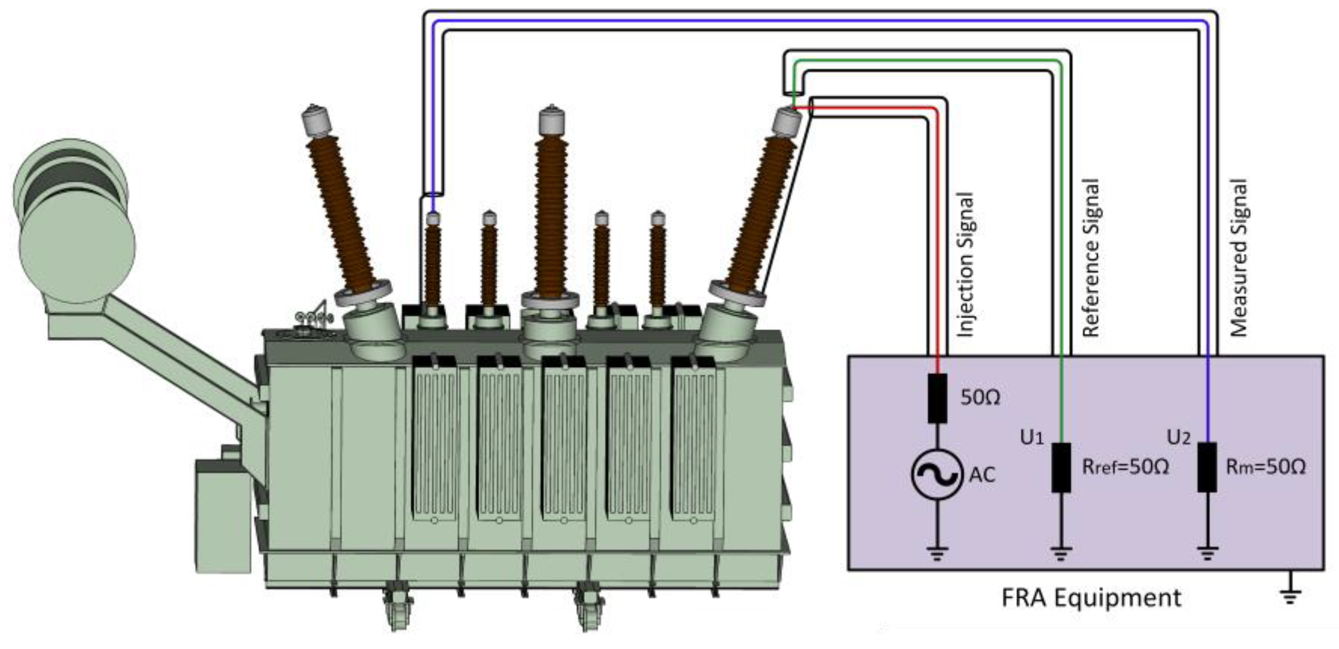
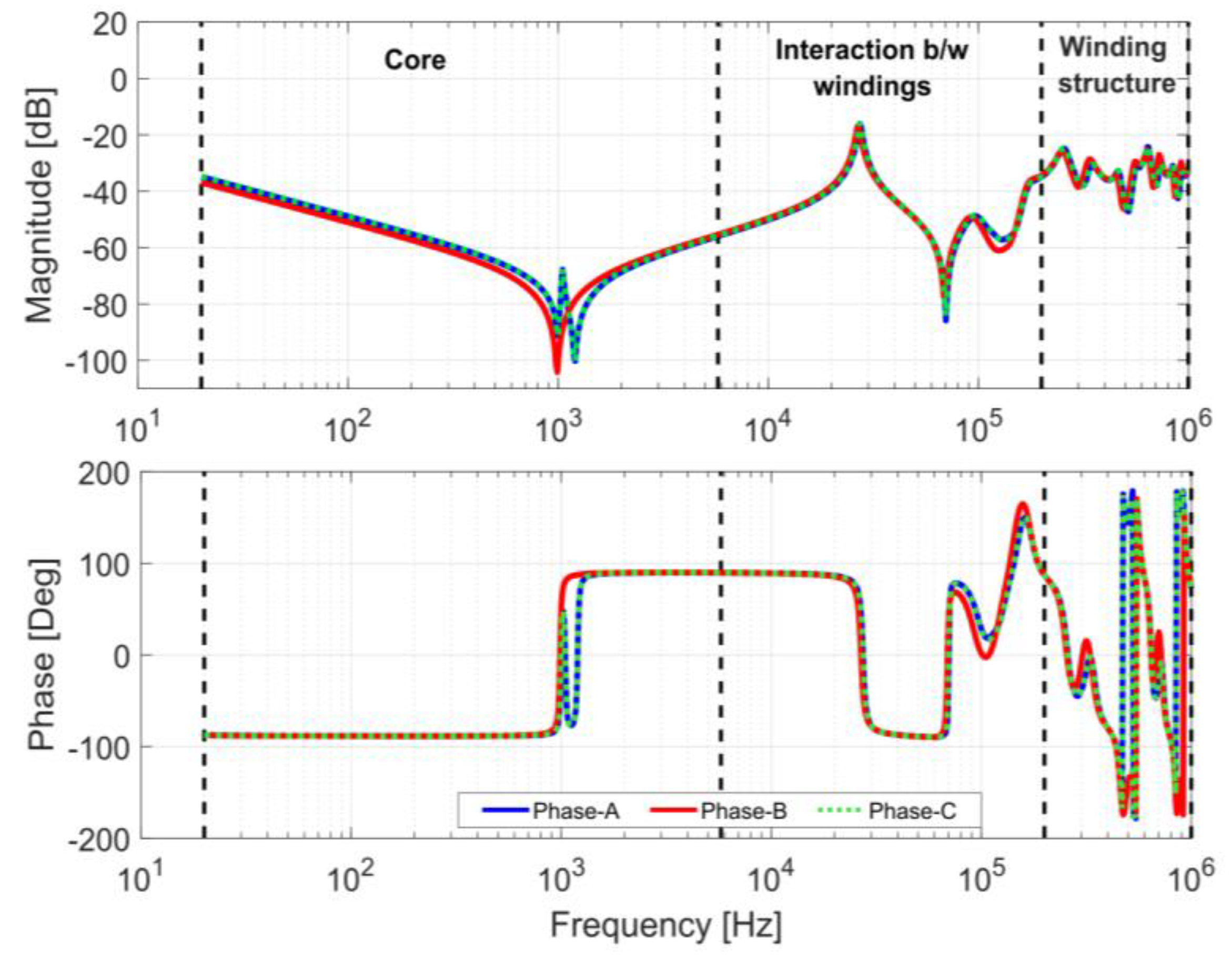
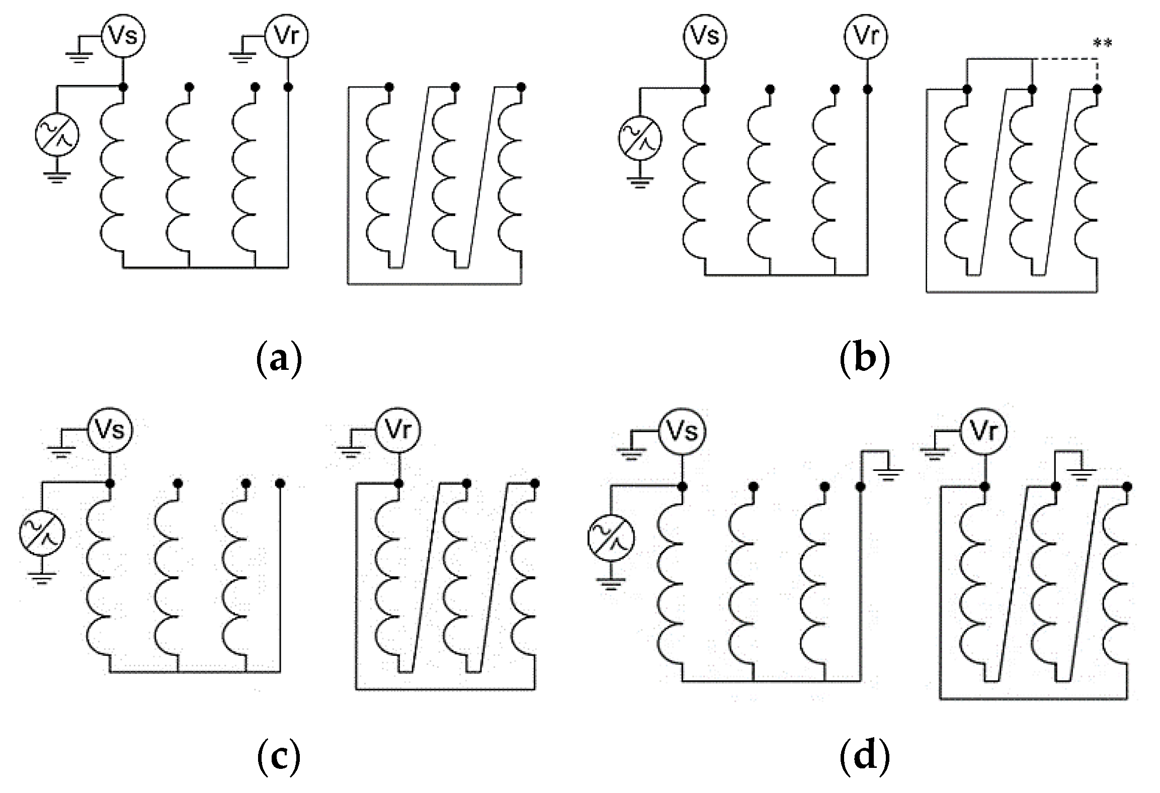
2. Principle of FRA

In FRA, transfer functions (TFs) of transformers are measured. TFs are determined by the electrical parameters of power transformers, such as capacitance and inductance of windings, capacitance between windings, capacitance between windings and ground, etc. This diagnostic method is based on the principle that the geometrical changes in the transformer core and windings due to mechanical stresses can be considered as a change in the RLC parameters of the equivalent circuit of the power transformer. Therefore, these changes can be detected through a change in the TF of the transformer. The measurement is performed over a wide range of frequency (few Hz to several MHz), and the results are compared with a reference measurement “fingerprint” of the winding to perform a diagnosis. The measurement setup for the FRA method is shown in Figure 1. A voltage signal of variable frequency is injected at one terminal, and the response is measured at the other terminal. The response will vary in magnitude and phase. The TF depends on the measurement resistance (50 Ω) and impedance of the transformer Z(ω), as expressed in Equation (1).

$$TF\left(\omega \right)=20log\frac{50}{50+Z\left(\omega \right)}$$

(1)

Figure 2 shows four connection schemes, i.e., end-to-end open circuit (OC), end-to-end short circuit (SC), capacitive inter-winding (CIW), and inductive inter-winding (IIW) as recommended by IEC standard [9].

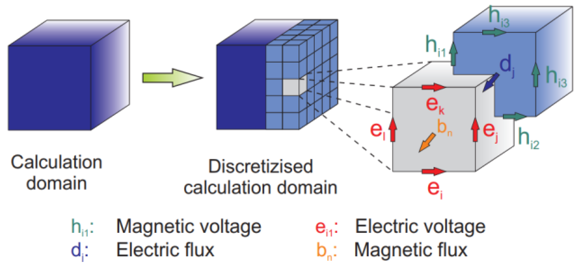
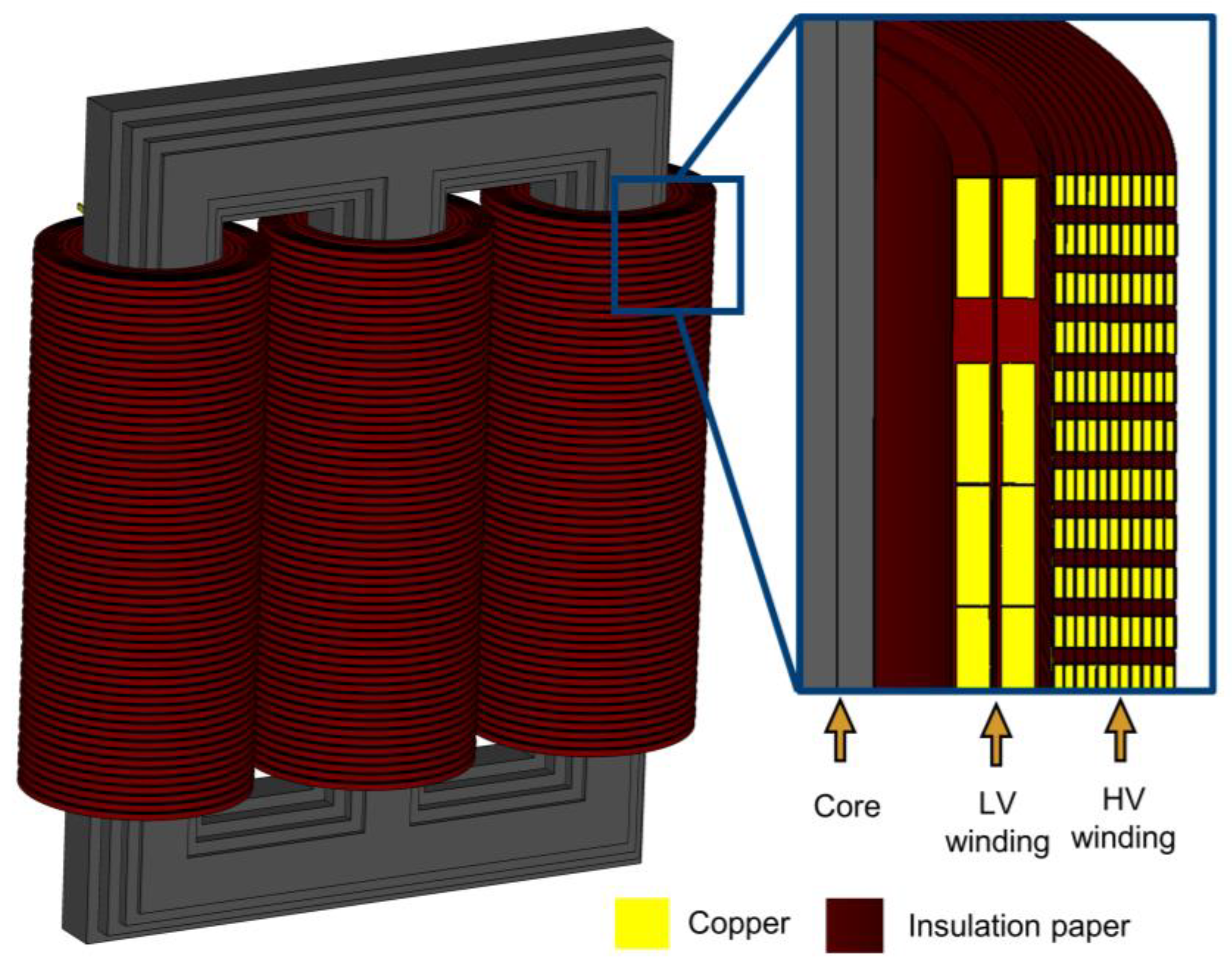
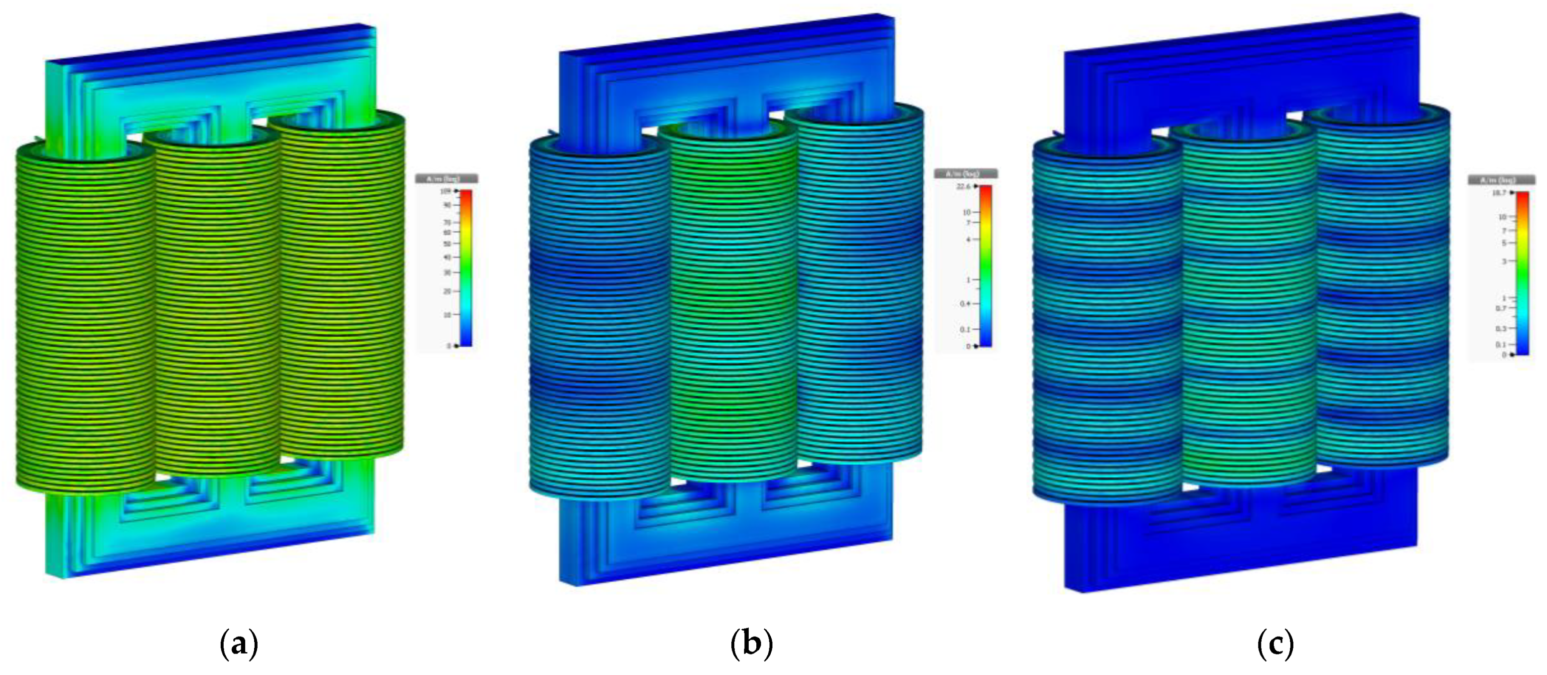
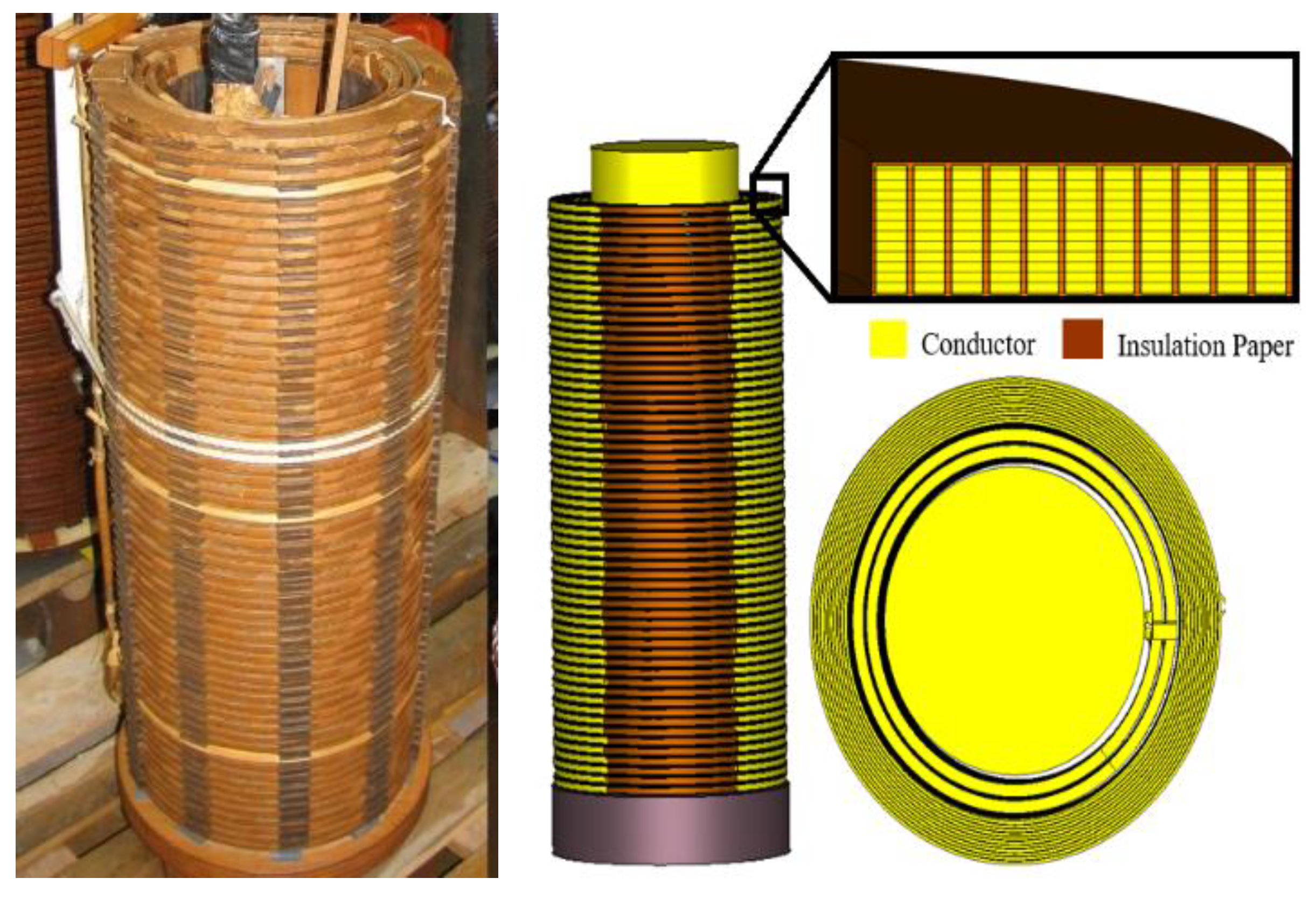
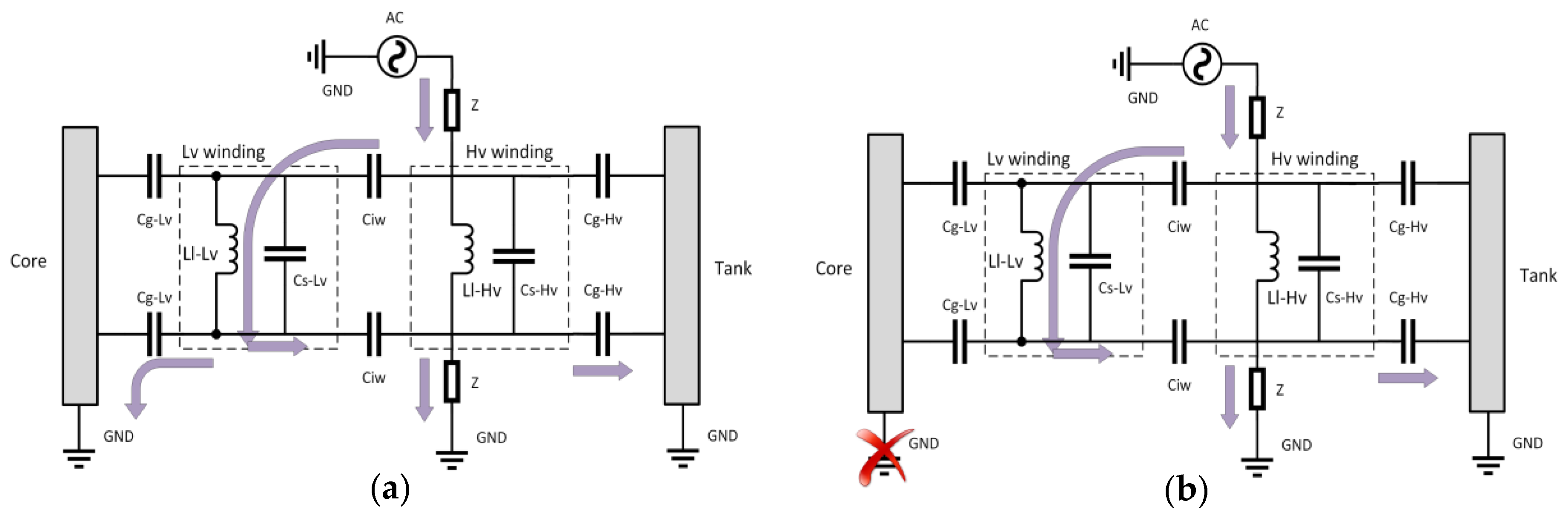
3. High-Frequency Transformer Modelling

The main idea of using a 3D high-frequency model is to emulate the real transformer and FRA measurement operations. CST Microwave Studio is used to model transformer behaviour and FRA measurement operations, which is based on the finite integration technique (FIT), first proposed by Weiland in 1977 [15]. FIT is a spatial discretization approach to numerically solve electromagnetic fields in the time and frequency domain and lead to a single solution. FIT is based on the integral form of Maxwell equations. In this method, a computational domain is spatially discretized by a doublet of two computational grids: primary grid $\mathrm{G}$ and dual grid $\tilde{\mathrm{G}},$ as shown in Figure 3. The electric voltages (e) and magnetic fluxes (b) are allocated on the primary grid while the magnetic voltages (h) and dielectric fluxes (d) are allocated on the dual grid. Finally, the spatial discretization of the continuous Maxwell equations is performed on this system of orthogonal computational grids. The discrete equivalent of Maxwell’s equations, the so-called Maxwell grid equations, are expressed as:

$$\begin{array}{ll}\mathrm{C}\widehat{\mathrm{e}}=-\frac{d}{dt}\widehat{\widehat{\mathrm{b}}}& \tilde{\mathrm{C}}\widehat{\mathrm{h}}=\frac{d}{dt}\widehat{\widehat{\mathrm{d}}}+\widehat{\widehat{\mathrm{j}}}\\ \mathrm{S}\widehat{\widehat{\mathrm{b}}}=0& \tilde{\mathrm{S}}\widehat{\widehat{\mathrm{d}}}=\mathrm{q}\end{array}$$

(2)

In these equations, C, $\tilde{\mathrm{C}}$, S, and $\tilde{\mathrm{S}}$ are the topological matrices representing the discrete equivalents of curl and div operators; the tilde matrices belong to the dual grid.

In this paper, a turn-based 3D high-frequency model of a three-phase 3 MVA transformer is developed, which consists of HV and LV windings, including the insulation papers as well as core and surrounding tank, as shown in Figure 4 (tank: hidden). The HV winding is a continuous disk winding with 660 turns in 60 disks, and the LV winding is a helical winding with 24 turns and 12 parallel conductors in each turn. In Appendix A,

Table A1. Geometrical dimensions of the three-phase transformer.

Parameters	Details
LV winding	Layer winding: 24 turns, 12 parallel conductors in each turn
HV winding	Disc winding: 60 discs, 11 turns in each disc
Radius of core	10.5 cm
Inner radius of LV	11.5 cm
Inner radius of HV	14.57 cm
Height of core	134 cm
Windings height	85 cm
Tank height	136 cm
Tank width	52.8 cm
Tank length	132 cm
Employed vector group	YNyn0

lists the parameters and geometrical details of the transformer. The 3D electromagnetic (EM) simulations were performed in a high-frequency solver of CST MW STUDIO [16]. It solves the discrete Maxwell equations in frequency-domain and calculates the electric and magnetic field distributions at different frequencies; hence, it considers the frequency-dependent effects in the core and volume of the conductors. In order to simulate the behaviour of the ferromagnetic core, frequency-dependent anisotropic complex permeability is considered. The real and imaginary parts of the complex permeability represent the ability of the core material to conduct the magnetic flux and the losses generated in the core due to eddy currents, respectively. As turn-based geometries of the windings are considered, thus, the HF model provides an accurate determination of turn-based parameters, i.e., self-inductance of each turn, mutual inductance between coils, inter-turn, and inter-disc capacitance, etc. The frequency-dependent losses, such as eddy current effects (skin and proximity effect) in the coils and dielectric losses in the insulation structure, are also considered.

For each 3D EM simulation setup inside CST MW STUDIO, two fundamentally different modules exist, i.e., the design module and the schematic module. In CST, FRA simulation is a three-step process. Figure 5 explains the flowchart of the algorithm for FRA simulation. Firstly, a 3D turn-based geometric model is created in the design module. Secondly, the broadband frequency-domain electromagnetic field computations are performed in the high-frequency solver where the excitation ports are set at both ends of the windings. The model is discretized by applying tetrahedral mesh. The output of this stage is a multiport-network, which characterizes the electromagnetic properties of the 3D geometry model. For a three-phase transformer, a twelve port network model is obtained. Lastly, the multi-port network is applied to the schematic module, where a sinusoidal voltage source is applied analogously to the real FRA measurements to calculate the FRA traces for different connection schemes. In this way, the FRA traces are directly obtained from the 3D high-frequency model of windings without estimating and solving the lumped parameter circuit models.

Figure 6 displays the magnetic field strength at different frequencies, i.e., 20 Hz, 500 kHz, 1 MHz. As can be seen, the magnetic field strength decreases with the increase of frequency. At low frequency, flux penetration in the conductor (winding and core) is high. However, as frequency increases, eddy currents are induced in the conductor (winding and core). Consequently, the flux will be confined to the thin layer near the surface, which reduces the magnetic field strength. Note, at 500 kHz and 1 MHz, the flux penetration into the core reduces significantly. Thus, the high-frequency components do not contribute appreciably to the flux in the transformer core, as mentioned in [17]. The Open-circuit frequency response of high voltage winding (HV-OC) of the HF model for open circuit configuration in a healthy state of the windings is shown in Figure 7.

The presented HF model gives manifold advantages in calculating the frequency response of the transformer. First, the HF-model considers the frequency-dependency of the winding parameters. Second, transfer functions are calculated directly from the 3D winding model without conversion and solving lumped parameter circuit-models. Third, various mechanical faults that are difficult to implement in circuit models can also be simulated in the presented HF model. Lastly, the frequency response of different types of windings, and various vector-groups can be analyzed. In addition, it is also possible to study the effects of windings different electrical properties on the frequency response of the transformer. For instance, it is possible to change the permittivity and dissipation-factor of the oil-paper to simulate the different moisture levels. A study on moisture-content identification in a small test setup has been performed [18], but the model proposed in this paper can be easily employed for such a study to model different transformer windings with different constructions. Additionally, the proposed model is also useful to study the transient analysis of power transformers, and calculation of winding overvoltages under different fault conditions. These studies are the future steps for developing and enhancing the application of the proposed HF transformer model.

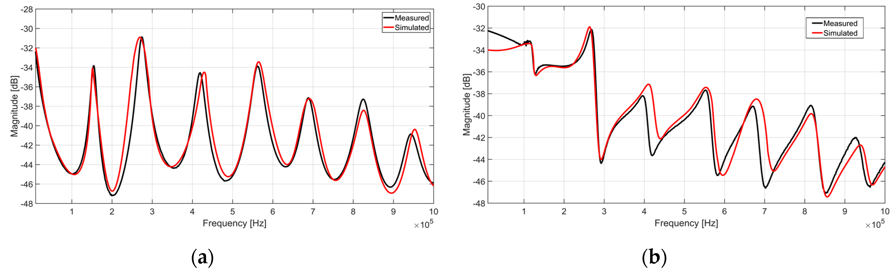
4. Validation of 3D HF Transformer Model

The method is validated with a simple experimental setup, which consists of HV and LV windings. The windings correspond to a medium voltage transformer of 1 MVA. The HV and the LV windings are similar to the three-phase HF model of the transformer, as described in Section 3. In this setup, two hollow copper cylinders are employed outside and inside of the windings to model the tank and the core, respectively. The experimental setup and the corresponding CST MW Studio model are shown in Figure 8. The model was validated with measurements for both healthy and deformed state of windings, as shown in Figure 9 and Figure 10, respectively. These results are based on the author’s previous work in [19,20], with minor improvements. The performance of this method against different mechanical faults was also proven in [19,20]. Thus, detailed validation results are not included in this article; rather, only the results of axial displacement (AD) fault in the IIW connection scheme are presented here. Five steps of AD (each step = 10 mm) are implemented in the HV winding, in both the experimental setup and CST model. The simulation results are compared with measurements, as shown in Figure 10. The results show good principle agreement of the simulations with the measurements, which proves the applicability of the HF model for interpretation of transformer frequency response.

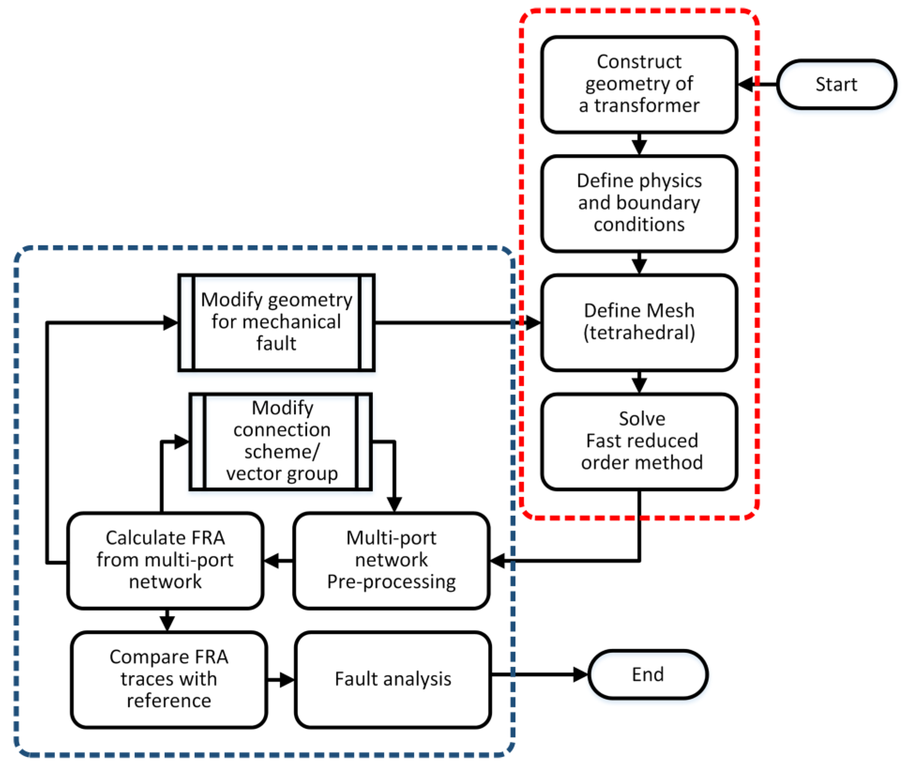
5. Evaluation Method

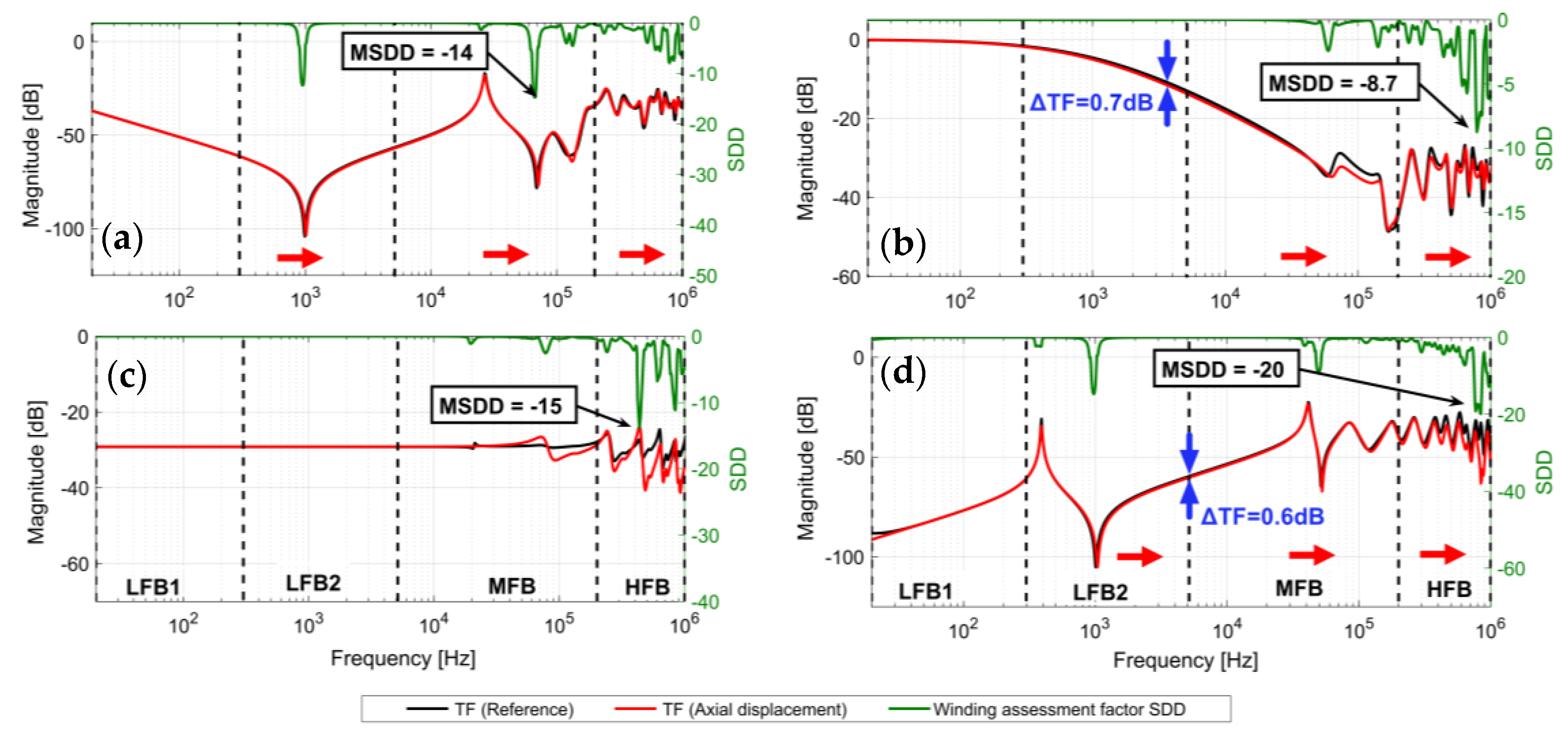
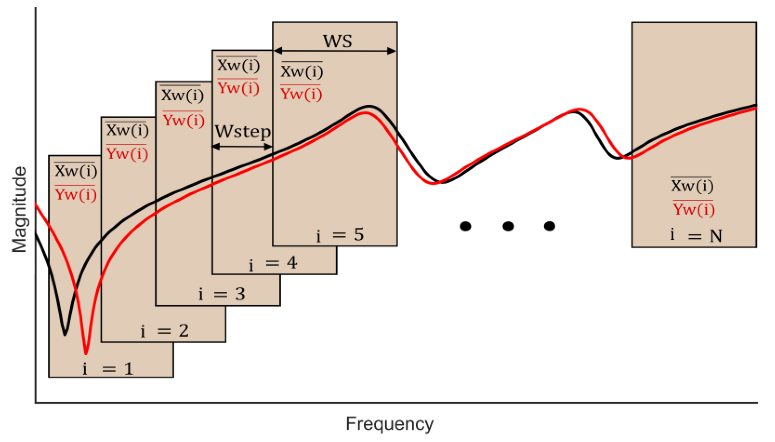
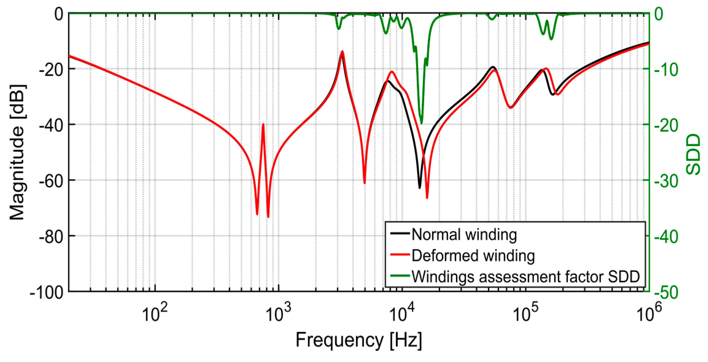
5.1. Transformer Winding Assessment Algorithm

In this study, a winding assessment factor is presented to compare TFs and quantify changes between them. The proposed method is based on the fact that the degree of deviation is quantified by evaluating the mean deviation of differences between two variables and this deviation is then standardized with the number of samples, and hence, called the standard deviation of difference (SDD). In this method, SDD is calculated in a window with a specific window size. This window is moved from the starting frequency to the ending frequency of the TF with a specific window step (Wstep = 1). In this way, the entire frequency spectrum of TF is scanned, and SDD is calculated in each window. Consequently, a vector is obtained characterizing the differences between two TFs as a function of frequency. Hence, the calculated SDD and measured transfer functions can be presented on the same graph. The winding assessment factor is calculated as:

$$\overrightarrow{SDD(i)}=-2\left(\sqrt{\frac{{\displaystyle {\sum }_{j=1}^{WS}{\left(Z(j)-\overline{Zw(i)}\right)}^2}}{WS-1}}\right)$$

(3)

$$\overrightarrow{Z(i)}=X(i)-Y(i)$$

(4)

$$\overline{Zw(i)}=\overline{Xw(i)}-\overline{Yw(i)}$$

(5)

$$\overline{Xw(i)}=\frac{1}{WS}{\displaystyle \sum _{j=1}^{WS}X(j)}$$

(6)

$$\overline{Yw(i)}=\frac{1}{WS}{\displaystyle \sum _{j=1}^{WS}Y(j)}i=1,2,3\dots N$$

(7)

$$WS=10+6\left(\frac{f_{res}-200}{200}\right)$$

(8)

where X and Y are the magnitude vectors of reference and measured TFs, respectively. X(i) and Y(i) are the ith elements of these vectors. $\overline{Xw\left(i \right)}$ and $\overline{Yw\left(i\right)}$ are the means of the ith window. f_res is the number of data points per decade, and WS is the window size. In the international standard IEC 60076-18 [9], the minimum measurement frequency resolution is specified, which is 200 points per decade. To take into account the effect of different frequency resolutions, window size is made variable and is calculated from Equation (8). In this way, the effect of different frequency resolutions is also considered. Figure 11 illustrates the basic principle of the presented method. While the representation of the proposed method for identification of the degree of deviation between two TFs of a three-phase transformer is shown in Figure 12. It can be seen that the proposed method has the following advantages:

• Increased fault detectability;
• Removes the issue of fixed frequency sub-bands for FRA interpretation;
• Plotting deviation between two TFs as a function of frequency;
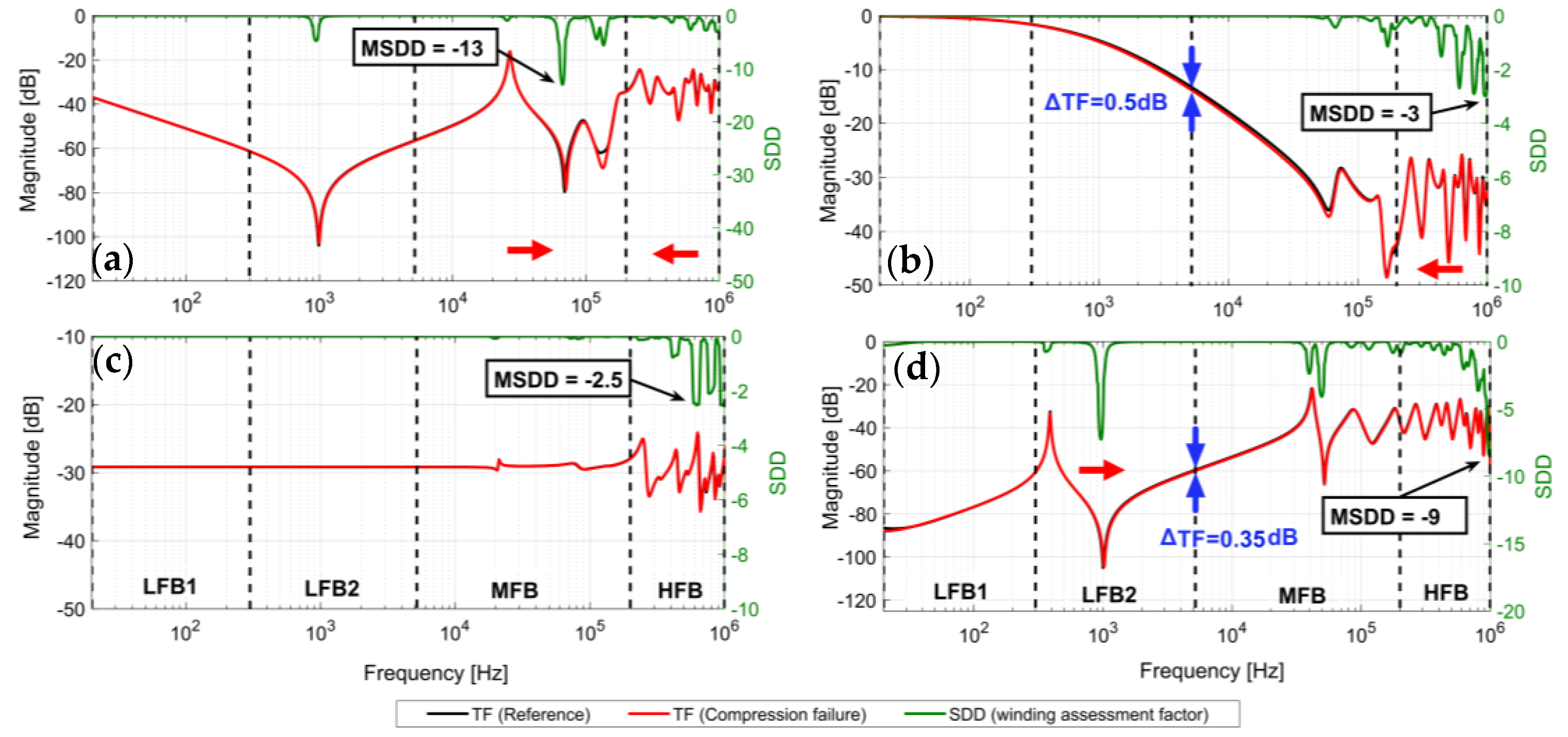
• Possibility to set a threshold to the lowest value of SDD function, i.e., MSDD;
• Possibility of faults classification.

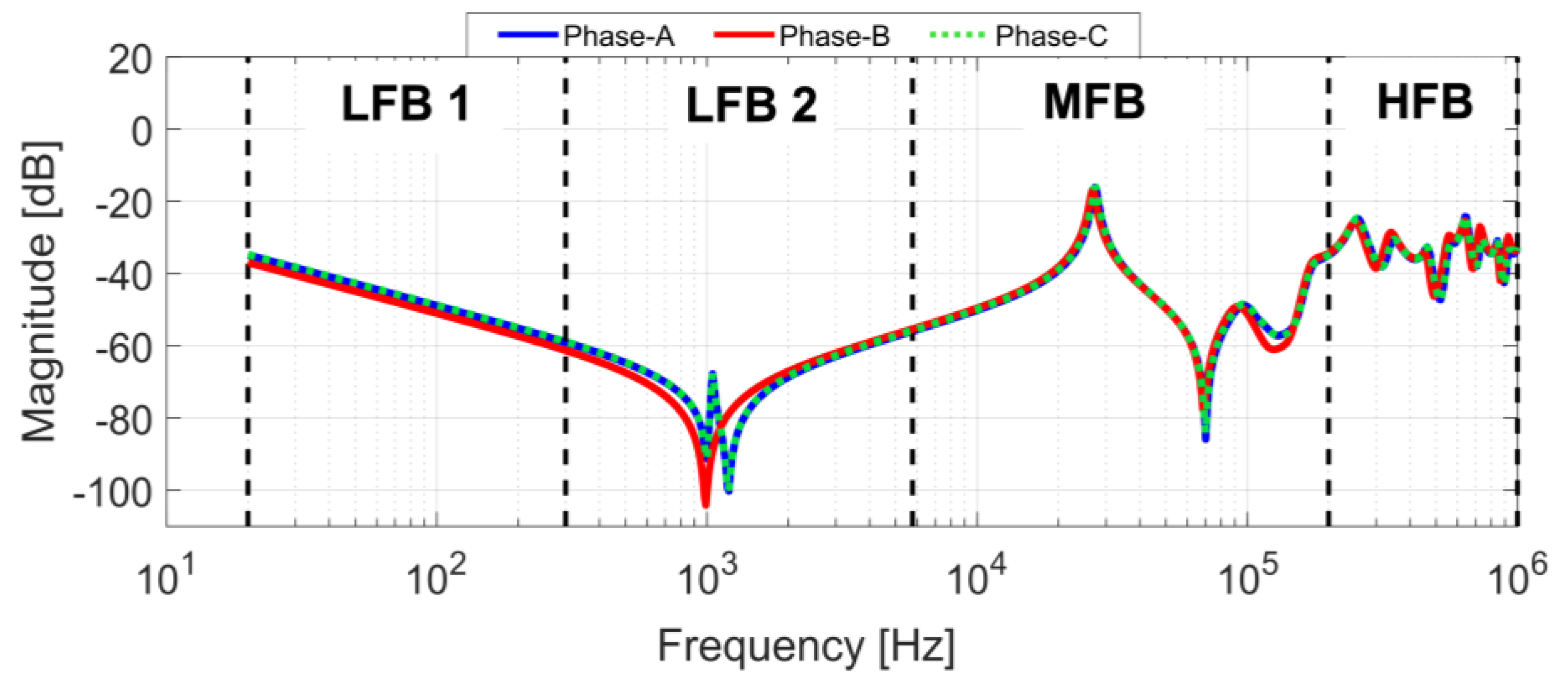
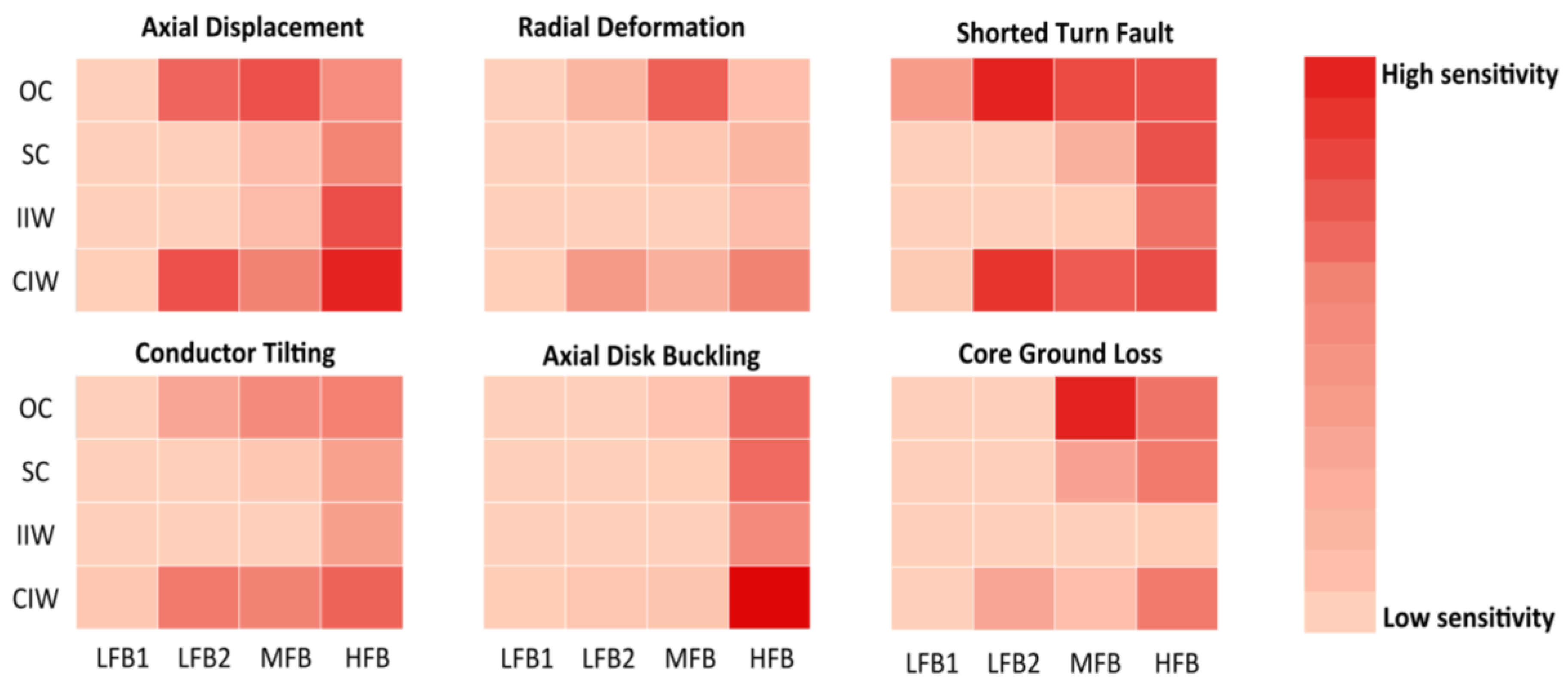
5.2. Division of Frequency Sub-Bands for Fault Classification

Since the frequency response of a transformer has a fundamental relationship with core and winding structure. Consequently, faults related to different components are dominated in different frequency regions. In this way, different faults can be classified by a proper definition of frequency sub-bands structure in the FRA spectrum. For fault classification, this contribution suggests a frequency sub-band structure, which divides the entire FRA spectrum into four regions, i.e., low-frequency1 (LFB1), low-frequency2 (LFB2), medium-frequency (MFB), and high-frequency (HFB). These frequency sub-bands are linked to different physical components of the transformer. For example, two low-frequency sub-bands (LFB1 and LFB2) are related to the core where magnetizing inductance (Lm) and equivalent network capacitance (Cnet) dominates. Medium frequency sub-band (MFB) is dictated by the mutual inductances between windings (Mu) and inter-winding capacitances (Ciw). While the high-frequency region is controlled by the winding structure. Figure 13 illustrates the four-frequency sub-band structure for a transformer winding. It should be noted that this frequency division is based on the open-circuit (OC) transfer functions. It is important to mention that the limits of these sub-bands depend on the physical size and rating of the transformer [8,9]. The frequency sub-bands shown in Figure 13 are only used for discriminating the low, the medium and the high-frequency sub-bands for the particular transformer windings in the example.

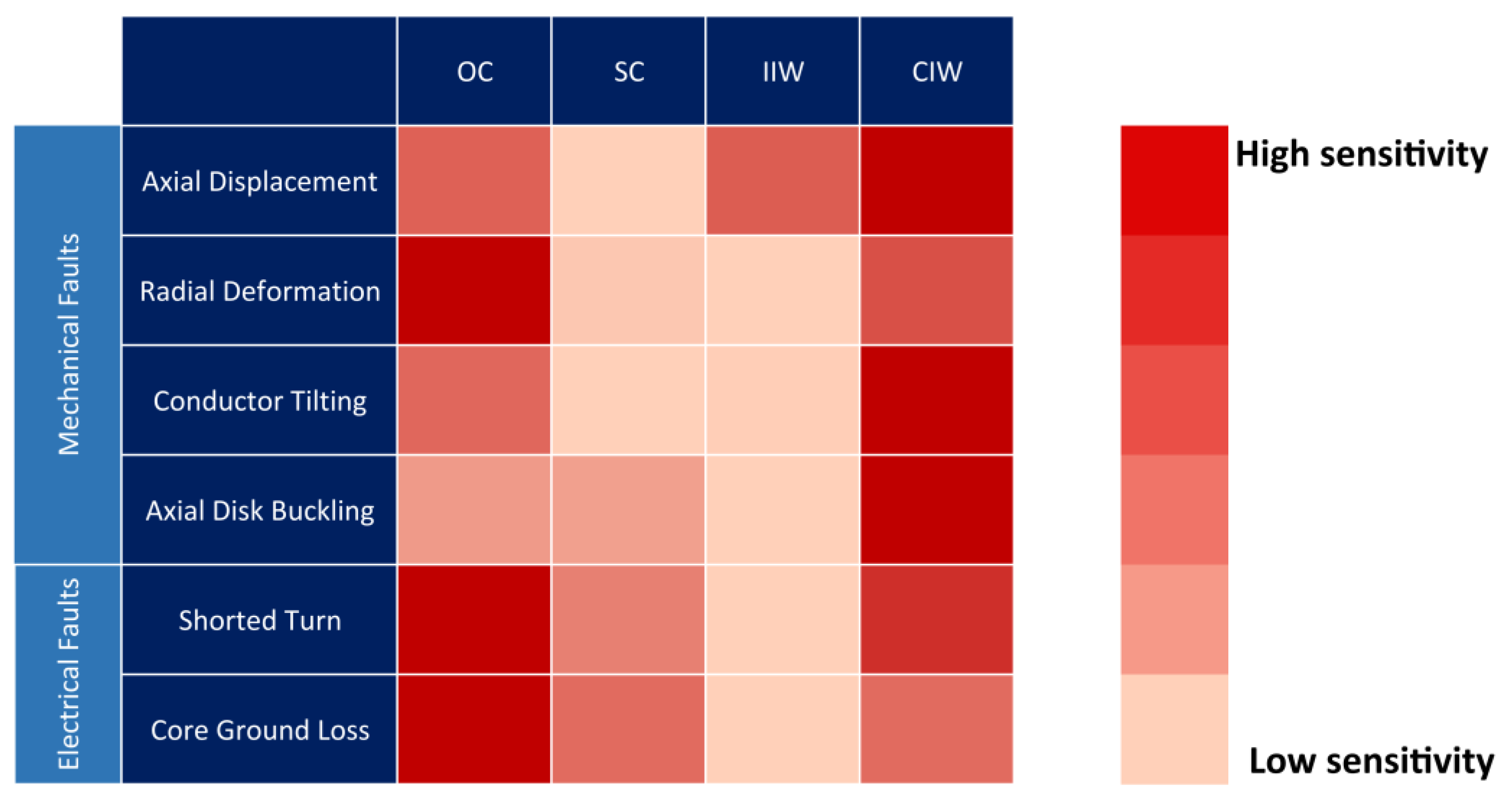
6. Fault Mechanism in Transformer Windings

Transformer winding faults are typically caused due to mechanical and/or electrical changes inside the transformer. Mechanical changes can arise during the short-circuit events (generating large electromagnetic forces), transportation, installation and/or service life, etc. Among these, the failures due to the generation of electromagnetic forces are most common. The electromagnetic forces are resolved into two components, i.e., radial and axial. The radial (axial) forces are generated by the interaction of short-circuit current and axial (radial) components of the leakage flux density, as shown in Figure 14. These massive electromagnetic forces can displace or deform the windings. The radial forces act inwards on the inner winding producing compression failure, and they act outwards on the outer winding producing hoop tension failure [21]. While the axial forces are generated parallel to the height of the winding, and they act in the opposite direction due to the pattern of the magnetic field. These opposing forces can be of two types, i.e., axial compression forces and axial expansion forces. Axial compression forces directed axially towards the windings centres and can collapse the winding. Axial expansion forces directed axially toward the top and bottom clamping plates and can bend or break them, allowing axial instability [21]. While electrical changes, i.e., shorted-turns, open circuit, can be caused due to ageing and/or subsequent of a mechanical failure.

In this paper, mainly, the effects of two fault classes are investigated, i.e., mechanical faults and electrical faults. In the category of mechanical failure modes, four common failure modes are simulated, i.e., axial displacement, axial disk buckling, conductor tilting, radial buckling (compression and hoop buckling). While in the class of electrical failure modes, two common failure modes, including short-circuit between turns and core ground loss, are investigated. The details of each simulated fault and its effect on FRA spectrum is discussed in the section below:

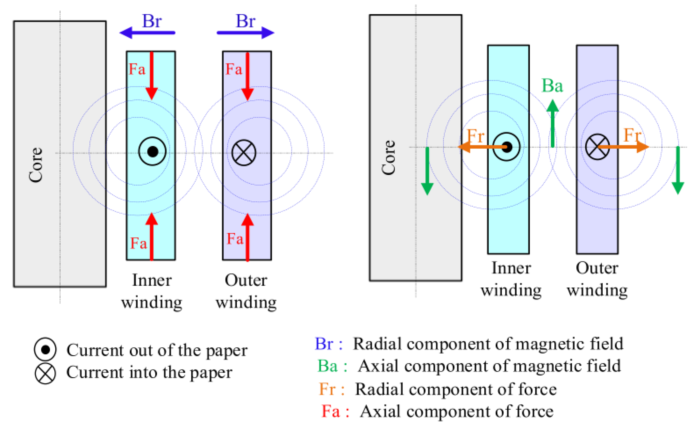
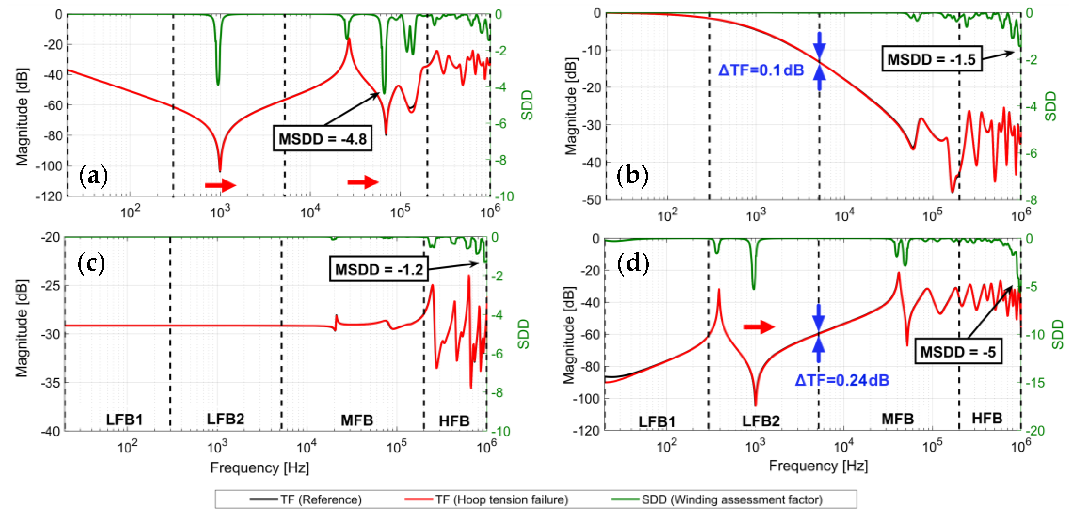
6.1. Mechanical Failure Modes

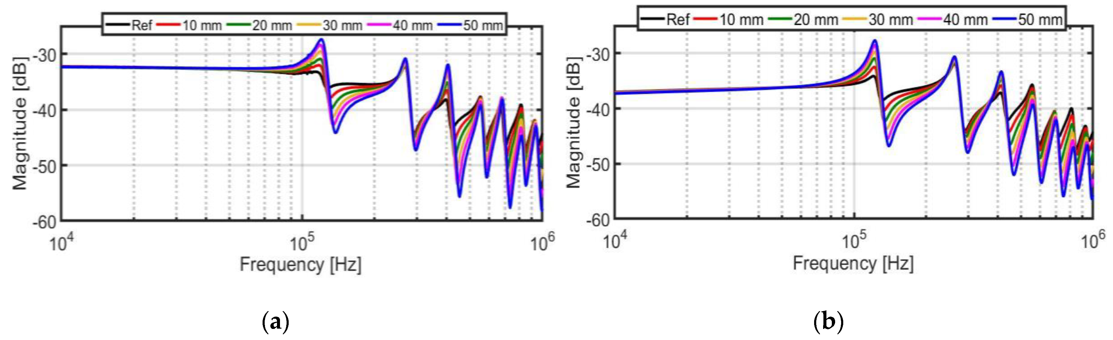
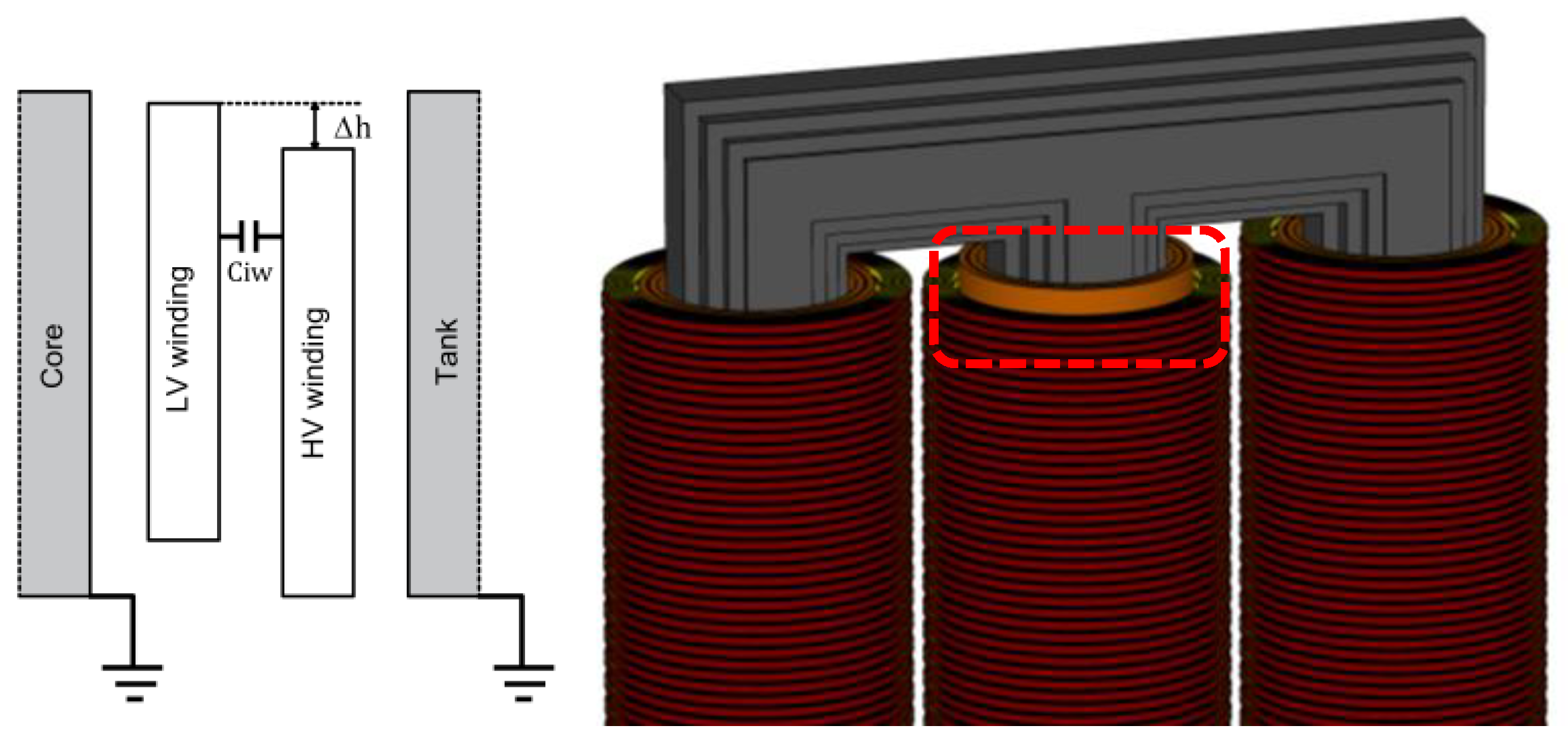
6.1.1. Axial Displacement Fault (ADF)

Axial displacement of windings is one of the most severe mechanical faults in power transformers. Any mechanical failure of the clamping system would allow windings to move in opposite vertical directions relative to one another; it is also referred to as bulk winding movement or telescoping [21]. A schematic representation of the ADF, in a typical transformer winding, is shown in Figure 15. To simulate ADF, the HV winding of B-Phase is displaced downward by ∆h = 30 mm (~3.5% of its height), as shown in Figure 15. Due to the courtesy of the multiport network, it is possible to connect the 3-phases of the model in different vector groups. In this paper, the TFs of the YNyn0 vector group are simulated. To discuss the sensitivity of different connection schemes, four connection schemes, i.e., OC, SC, CIW, and IIW, are implemented. Figure 16 shows the effect of ADF on TFs of four connection schemes. Under ADF, the interaction of the windings and hence the mutual couplings (Ciw and Mu) are changed. Consequently, the effects of ADF are mainly appreciable in the MFB and HFB. Moreover, it can be seen that the impact of ADF is different in different connection schemes and is briefly explained in the following:

HV-OC: TF remains unchanged in LFB1. In LFB2, the first anti-resonance point is slightly shifted to the right due to the decrease of the Ciw. The effect of ADF is most obvious in the MFB and HFB, where the resonance frequencies are shifted to the right due to the decrease of Mu and Ciw.

HV-SC: The effect of ADF can be perceived in the inductive roll-off region. In this region, due to the change of impedance, the difference in TFs of healthy and affected winding is 0.7 dB. In MFB and HFB, the effect of ADF is similar to HV-OC configuration.

IIW: TFs in LFB1 and LFB2 give a measure of the turns ratio, and it remained unaffected under ADF. While TFs in MFB and HFB are significantly changed, new resonance peaks and valleys are observed.

CIW: The low frequency (LFB1 and LFB2) response of this configuration shows a linear behaviour that is dominated by Ciw. Due to the decrease of Ciw, the TFs are shifted downward with a change of 0.6 dB. Also, the resonance frequencies are shifted to the right due to the decrease of Ciw and Mu. The deviation between TFs is maximum in HFB.

In Figure 16, the calculated SDD is also plotted as a winding assessment factor, which gives a quantitative measure of deviation between TFs. The minimum value of SDD (MSDD) indicates the maximum deviation between TFs. It can be seen that TFs of inter-winding configurations (IIW and CIW) possess the lowest value of SDD, indicating that these configurations are more sensitive to ADF.

6.1.2. Radial Deformation Fault (RDF)

Mainly, two types of radial deformations can be found, i.e., compression failure in inner windings and hoop tension failure in outer windings. Generally, the term “buckling” is used for both types of radial deformations [21]. However, their effects on the FRA spectrum can be different in different cases. In the HF model, both modes of radial deformation are implemented, as shown in Figure 17. For this purpose, one section of the B-phase winding is deformed throughout the winding height. Considering Figure 17, the radius of the radial deformation (r) is modelled as given:

$$r(\theta )=\{\begin{array}{ll}{r}_0-\frac{d}{2}(\cos (s\theta )-1)& 0\le \theta \le \frac{2\pi }{s}\\ r_0& \mathrm{otherwise}\end{array}$$

(9)

where, r₀ is the non-deformed radius, d is the deformation depth (positive d: compression failure of LV winding and negative d: hoop tension failure of the HV winding), s is the span of radial deformation, θ is the arc angle. The arc angle of the deformed section is kept at 30°, and the RDF level is calculated based on the depth of deformed and the non-deformed radius of the winding as follows:

$$\%\mathrm{RD}\mathrm{fault}\mathrm{level}=\frac{d}{r_0}\times 100\%$$

(10)

In the HF model, the RDF level of 10% and 5% is simulated in compression failure and hoop tension failure, respectively. The effects of both types of buckling on simulated FRA signatures for four connection schemes are shown in Figure 18 and Figure 19, respectively. To identify the degree of deviation between TFs, SDD is also displayed on the same graph. Under RDF, the distance of the winding to the ground (Cg: capacitance to ground), the interaction between windings (Ciw and Mu), the leakage inductance (L) and winding’s series capacitances (Cs) are changed. Consequently, the effects of RDF are noticeable in the MFB and HFB. It can be noticed that the impact of both types of bucklings is quite similar, as both affect the similar transformer winding parameters. The impact of buckling fault in different connection schemes is briefly explained in the following:

HV-OC (Figure 18a and Figure 19a): For both types of buckling, the LFB1 is unchanged. In LFB2, the first anti-resonance point is slightly shifted to the right (represented by the red arrows) due to the change of Cg, Ciw, and Cs. The deviations are most obvious in the MFB where the resonance frequencies are shifted to the right due to the decrease of Ciw and Mu. Small deviations at resonance points were also found in HFB, as detected by SDD. These changes can be attributed to the change of Cs.

HV-SC (Figure 18b and Figure 19b): For both types of buckling, TFs are changed in the inductive roll-off region. In this region, due to the change of leakage inductance, a change in TFs is observed. The difference in magnitude is 0.5 dB and 0.1 dB for compression and hoop tension failure, respectively. In HFB, both faults result in slight frequency and magnitude shifts.

IIW (Figure 18c and Figure 19c): TFs in LFB1 and LFB2 remained unaffected under both types of bucklings because RDF does not affect the turns ratio. In HFB, TFs are slightly changed, as indicated by SDD.

CIW (Figure 18d and Figure 19d): The linear behaviour of TFs in LFB1 and at the end of LFB2 is dominated by the capacitance between windings (Ciw). Due to the decrease of Ciw, the TFs are shifted downward.

By comparing the values of MSDD in different connection schemes, OC and CIW configurations can be identified as the most sensitive configurations to detect the RDF. In IEEE std. C57 [8] and CIGRE-342-2008 [22], few case studies regarding compression failure in inner winding are reported. The simulation results of the HF model show similar trends.

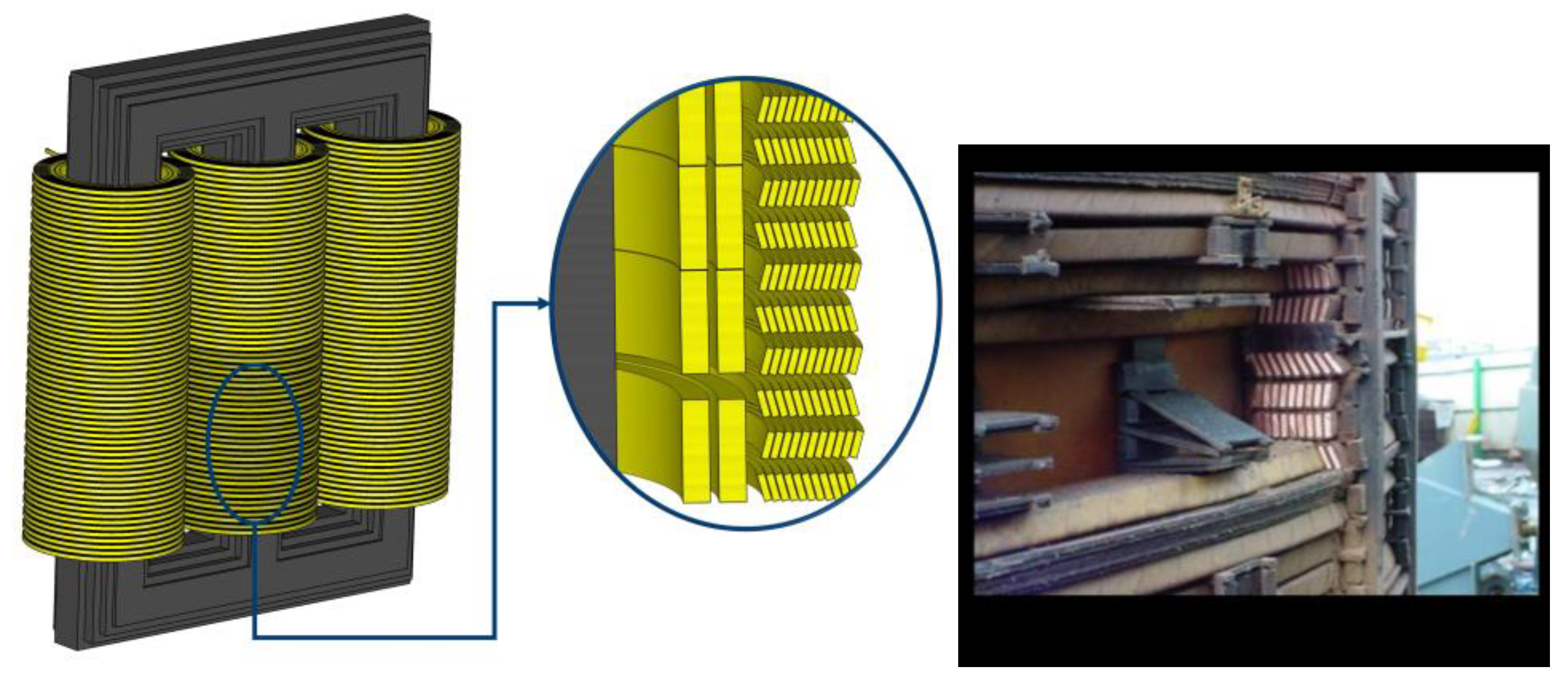
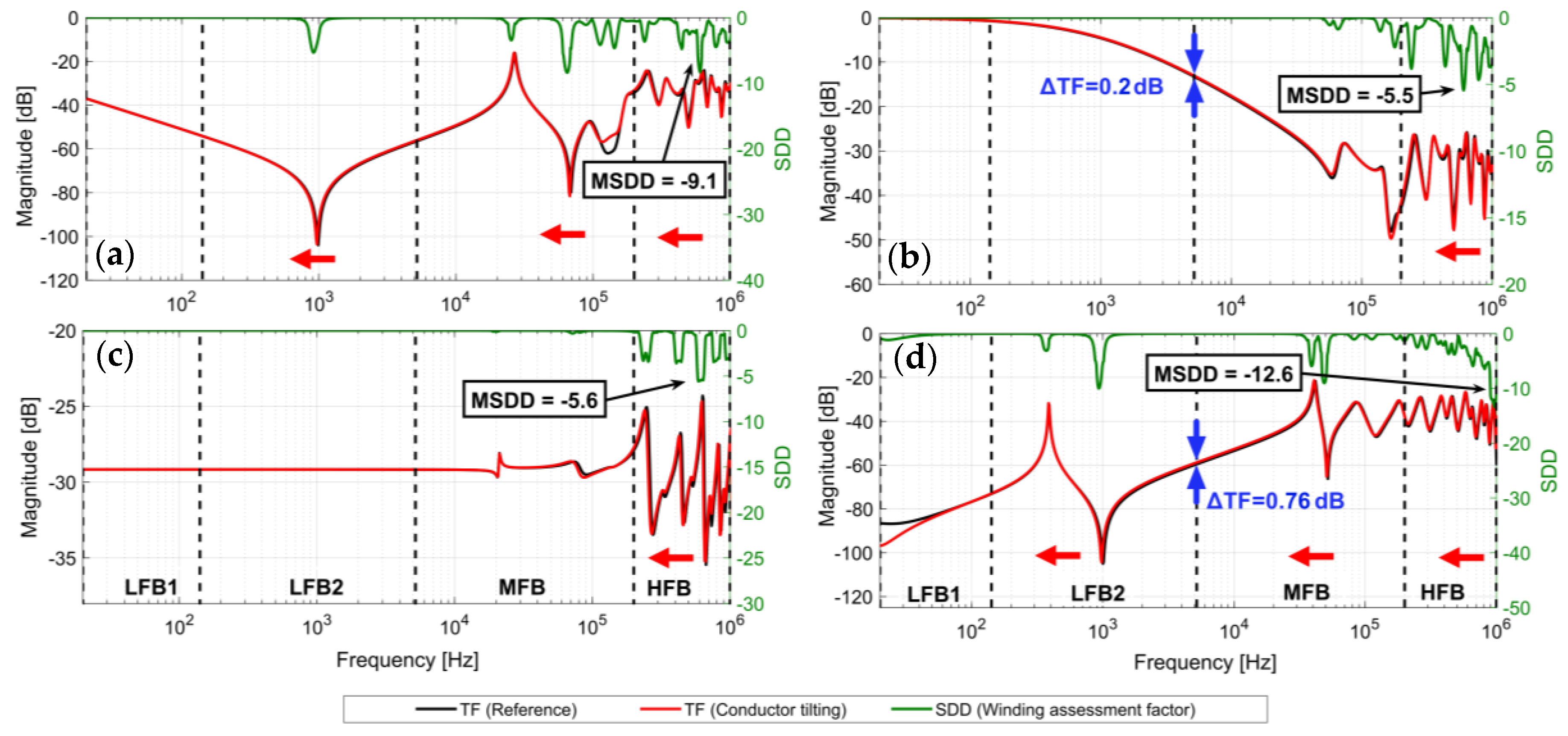
6.1.3. Conductor Tilting Fault (CTF)

In electromagnetically balanced windings, the axial forces act to axially compress the windings. When the axial compression force exceeds a certain limit, a fault called “conductor titling” occurs, which is a principal mode of failure in large power transformers [21]. In this mode of failure, the conductors turn around their axis of symmetry. The conductor tilting fault may result in damage to insulation paper, displacement of conductors, shorted-turn fault and even collapse of the winding in severe cases. Figure 20 illustrates the CTF in real transformer winding [22] and its equivalent simulation in the HF model. Conductor tilting is simulated by tilting the conductors in the entire circumference of the B-phase HV winding. The angle of tilt is kept at 15°, whereas the maximum tilt angle is considered to be 90°. CTF is applied to the bottom 30 disks, and the fault level is calculated based on the number of discs with tilted conductors as follows:

$$\%\mathrm{CT}\mathrm{fault}\mathrm{level}=\frac{\mathrm{number}\mathrm{of}\mathrm{faulted}\mathrm{discs}}{\mathrm{number}\mathrm{of}\mathrm{total}\mathrm{discs}}\times \frac{\mathrm{applied}\mathrm{tilt}\mathrm{angle}}{\max \mathrm{possible}\mathrm{tilt}\mathrm{angle}}\times 100\%$$

(11)

In this way, 8% of the CTF is simulated in the HF model. The effects of CTF on simulated FRA signatures for four connection schemes are shown in Figure 21. To identify the degree of deviation between TFs, SDD is also displayed on the same graph. The impact of the CT fault in different connection schemes is briefly explained in the following:

HV-OC: The effect of CTF is mainly prevailed in HFB, as indicated by MSDD. In this region, the resonance frequencies are shifted to the left (indicated by red arrows). The shift in the resonance can be attributed to the change of Cs of the winding. Because CTF is caused by axial compression of discs, the separation between the conductors changes, which eventually changes Cs.

HV-SC: Due to the change in impedance, the TF of the affected winding exhibits an attenuation of 0.2 dB within the inductive roll-off region. In MFB, the effect is small and difficult to identify. While in HFB, the largest differences in TFs are produced, which is also evident from the minimum value of SDD.

IIW: The differences between TFs are noticeable in HFB, while other regions remain unaffected.

CIW: In the linear behaviour of TFs in LFB1 and LFB2, the TF of the affected winding is shifted upward. This change can be attributed to the change in the Cs and Ciw. Whereas in HFB, the resonance peaks and valleys are shifted, which is a key indicator of the dominant effect of Cs in this region.

Looking at the values of MSDD in different connection schemes, CIW proved to be the most sensitive connection scheme to detect the CTF. Very few studies are found in the literature as CT fault is difficult to implement. In CIGRE-342-2008, one case study is reported [22]. The simulation results of the HF model show similar trends against conductor tilting failure mode.

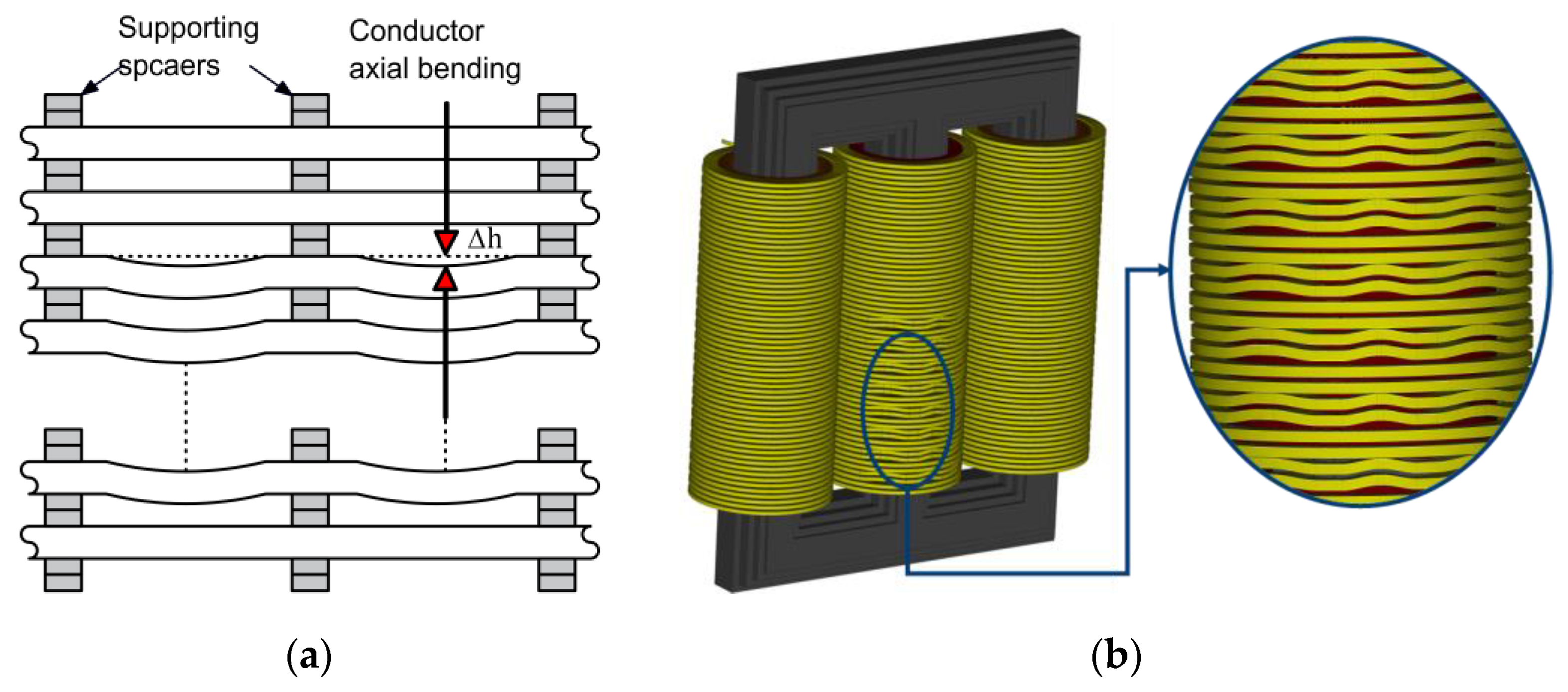
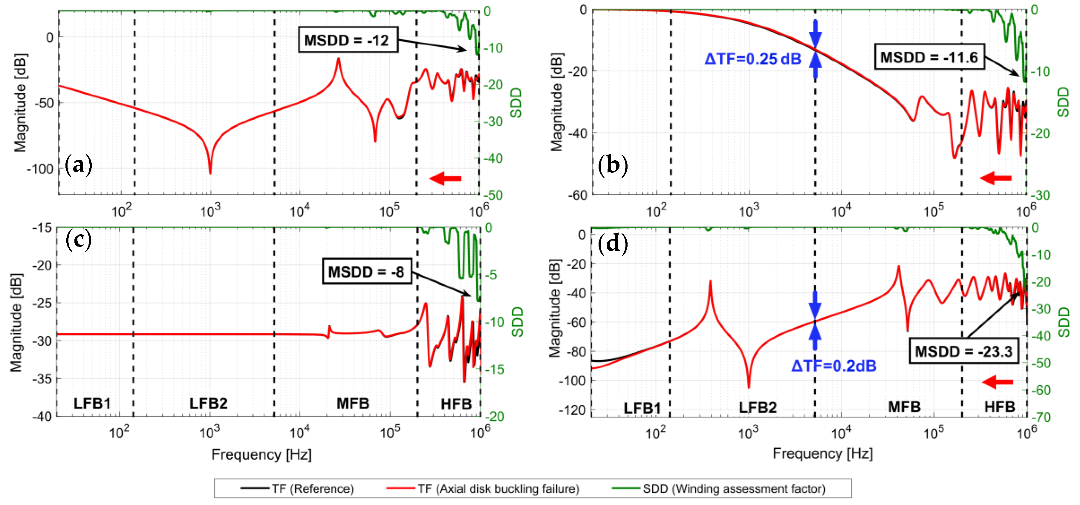
6.1.4. Axial Disk Buckling Fault (ADBF)

The opposing axial forces on the windings can also bend the conductors between insulating spacers, which are located radially or leaned to each other. The occurrence of this phenomenon is called bending or axial disk buckling. A schematic representation of the ADBF, in a typical transformer winding, is shown in Figure 22a. In the HF model, this fault is simulated by introducing a vertical buckling to the bottom 30 disks in HV winding, as shown in Figure 22b. The buckling distance (h) was set to 4 mm. While the distance (d) between normal disks was 5 mm. The arc angle of the deformed section is kept at 75°. The percentage ADBF level was calculated as follows:

$$\%\mathrm{ADB}\mathrm{fault}\mathrm{level}=\frac{\mathrm{number}\mathrm{of}\mathrm{faulted}\mathrm{discs}}{\mathrm{number}\mathrm{of}\mathrm{total}\mathrm{discs}}\times \frac{\mathrm{deformed}\mathrm{arc}\mathrm{angle}}{{360}^{\circ }}\times \frac{\mathrm{h}}{\mathrm{d}}\times 100\%$$

(12)

To study the impact of ADBF on TFs of different connection schemes, an 8% fault level is implemented in the HF model. The simulated TFs along with the application of winding assessment factor (SDD) is presented in Figure 23. The effects of ADBF in each connection scheme are briefly explained in the following:

HV-OC: Results do not lead to drastic deviations in LFBs and MFB as the value of SDD approaches to zero in these bands. ADBF only affects the winding structure. Consequently, the effects only appear in HFB where the resonance frequencies are shifted to the left (indicated by the red arrow). These effects are attributed to the changes in the inter-disk capacitance and Mu between the affected disks. The maximum change between TFs in HFB is also indicated by the minimum value of SDD.

HV-SC: The TFs of the affected case are offset in the inductive roll-off portion. In this region, due to the change of the impedance, the difference in magnitude is greater than 0.2 dB. In HFB, the effect is similar to the HV-OC.

IIW: TF of the affected winding is shifted to the left in HFB, recognized by the minimum value of SDD, while other frequency bands are unchanged.

CIW: In the linear behaviour of TFs in LFB1 and LFB2, the TF of the affected winding is slightly attenuated, but this change is minimal and difficult to identify. Whereas in HFB, the resonance peaks and valleys are shifted, which are also witnessed by the minimum value of SDD.

Looking at the values of MSDD in different connection schemes, CIW can be identified as the most sensitive connection scheme to detect the ADBF.

6.2. Electrical Faults

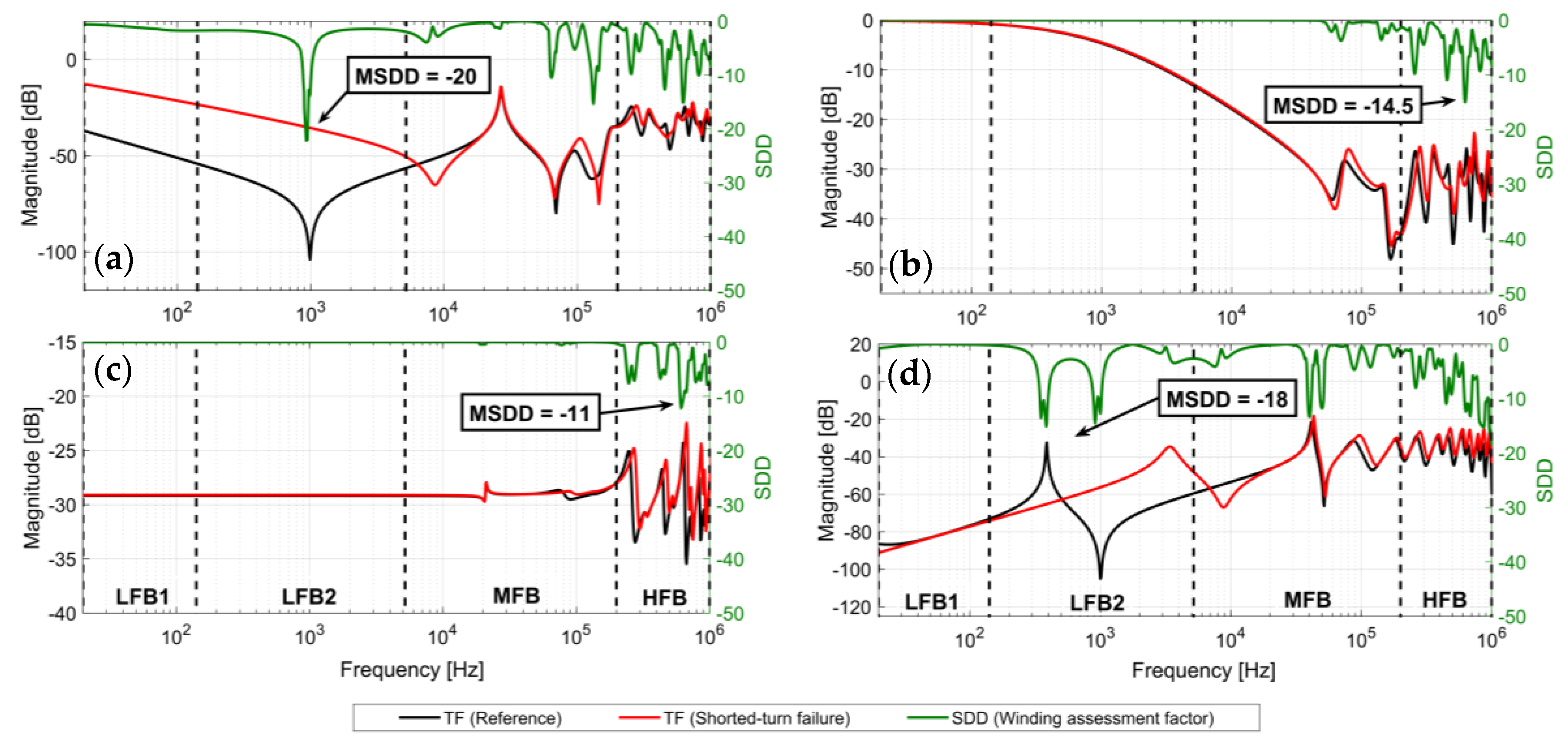
6.2.1. Turn-To-Turn Short Circuit Fault (TSCF)

Turn-to-turn short circuit is the most common electrical failure mode in transformer windings. Depending upon the severity, it can influence the characteristics of magnetizing inductance, winding resistance, and self-inductance of the windings. Shorted turn fault gives rise to large circulating currents, which leads to localized thermal overloading, thereby causing hot spots [21]. With the passage of time, the fault manifests itself and may lead to catastrophic failure of the transformer. In the HF model, TSCF is simulated by shortening two-turns at various locations in the B-phase HV winding. It was found that the shorted-turn fault in the middle of the winding has a greater impact on the TFs of the affected winding. This can be associated with the higher mutual inductance of the middle disks in comparison to the top and bottom disks. For this reason, only the results of one SC location (middle) are included in this paper. When a TSC fault occurs, a large amount of flux passes through the air instead of the core and surrounds the shorted-turn. Thus, the leakage flux is essentially increased at the fault location. Consequently, the magnetic reluctance and self-inductance of the corresponding limb changes. Figure 24 shows the impact of TSCF on simulated TFs of different connection schemes. To identify the degree of deviation between TFs, SDD is also displayed on the same graph. The impact of TSCF in different connection schemes is briefly explained in the following:

HV-OC: TSCF is most obvious in the low-frequency region. As stated earlier, the SCTF remarkably changes the magnetizing characteristics of the core and results in reduced magnetizing inductance. Consequently, TF of the affected winding is offset in LFBs, and the first resonance frequency is shifted up to 250% in comparison with the healthy case. Slight deviations can also be seen in the high-frequency region due to the change of the impedance of the winding.

HV-SC: Inductive roll-off region is affected due to the change of leakage inductance. In this region, a decrease in impedance is observed, and the difference in magnitude is greater than 0.2 dB. This region provides the possibility of a quantitative diagnosis of SCTF, and a diagnosis criterion can be set to a permissible change of the impedance. As the low-frequency response (inductive roll-off portion) of the short circuit configuration is equivalent to the short circuit impedance. According to IEC-2200-2014 [21], if the short-circuit impedance of a transformer changes by 2% or more, then the transformer is recognized as damaged. In MFB and HFB, new resonance peaks and valleys can be observed, which are also recognized by the SDD.

IIW: TFs in LFB1 and LFB2 are slightly offset due to the change in the number of turns. However, this change is minimal and difficult to identify, especially if fewer turns are shorted. In MFB and HFB, the resonance points are shifted, and new resonance peaks and valleys are produced.

CIW: In LFB2, the first resonance frequency is affected. While in MFB and HFB, the resonance frequencies are shifted to the right due to the decrease of the impedance of the winding.

From Figure 24, remarkable changes in the TFs of OC and CIW configurations indicate that these connection schemes are more sensitive to detect TSCF. Various studies related to the diagnosis of windings short circuit faults can be found in the literature. The presented simulation results of TSCF aligns well with the practical results reported in [8,9,22].

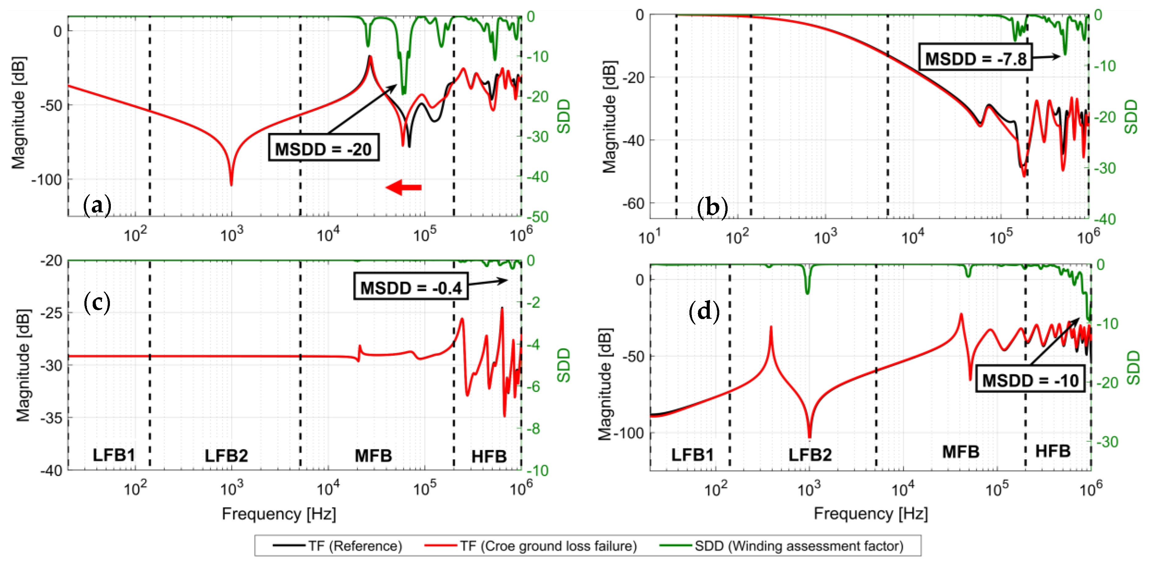
6.2.2. Missing Core Ground Fault (MCGF)

In the normal operation, transformer cores are tied to ground potential at one point. In case single point earthing is lost during transportation/service conditions, it will result in a heavy circulating current and cause excessive overheating of core, metallic parts, and leads connected to the earth. This is the most frequent event in the core and magnetic circuit failures [8]. Mostly, the connection to the ground of the core is made internally, thus making it difficult to simulate and understand the effect of the ungrounded core. In the HF model, it is possible to disconnect the core connection to the ground to study the impact of missing core ground on TFs of different connection schemes.

Generally, the missing core ground fault (MCGF) changes the LV winding-to-ground capacitance, which results in the shifting of the HV winding response in the medium and high-frequency range. This can be explained, using the circuit in Figure 25, where a simplified equivalent circuit of a two-winding transformer with and without core ground is shown. Under normal conditions, when the frequency response of the HV winding is measured by applying the voltage at the terminal of HV winding, the voltage will be induced in the LV winding, which is electromagnetically coupled with the HV winding. Consequently, at the measuring impedance, in addition to the HV winding current, there is a capacitive current flowing from LV winding. While in the case of a missing core ground, the coupling between the LV winding and ground is reduced, increasing the potential of the floating LV winding. This additionally increases the capacitive current flowing from LV winding through the measuring impedance. It will change the frequency response of the HV winding in the middle and high-frequency regions. Figure 26 shows the impact of MCGF on simulated TFs of different connection schemes. To identify the degree of deviation between TFs, SDD is also displayed on the same graph. The impact of MCGF in different connection schemes is briefly explained in the following:

HV-OC: The effect of MCGF is most obvious in the MFB and HFB. As mentioned earlier, MCGF results in additional capacitive current flowing from LV winding and inter-winding capacitances towards the measuring impedance. This capacitive component will change the TF of the HV winding in MFB and HFB. SDD also detects the larger differences between TFs in these regions.

HV-SC: The effect of MCGF is most prominent in the HFB where the resonance points are shifted, and new peaks and valley are produced.

IIW: This configuration is the least sensitive for MCGF. Slight differences between TFs appear in HFB. However, these differences are minimal and difficult to identify, as indicated by the minimum value of SDD (MSDD = −0.4).

CIW: At low frequency, inter-winding capacitance dominates the response, and a very slight deviation exists due to the change of ground capacitance that affects the inter-winding capacitance. The influence of missing core is increased at high frequencies around 1 MHz.

From Figure 26, the lowest value of MSDD in OC indicates the higher sensitivity of this configuration. It was also observed that this failure mode affects the TFs of all the phases.

Figure 27 summarises the characteristic impact of individual faults on the TFs of four connection schemes, i.e., OC, SC, CIW, and IIW. These deviation patterns are based on the minimum value of SDD (MSDD) in different frequency sub-bands for each fault type. Based on the presented case studies of mechanical and electrical failure modes, it can be observed that different patterns of deviations can be characterized for different faults according to the frequency sub-bands. Consequently, it is possible to classify different faults based on their deviation patterns in various frequency sub-bands. Thus, it can be summarized from the above case studies that the SDD indicator has the ability to detect and identify the fault types using the proposed frequency sub-band division structure. These deviation patterns can be served as features to train and develop an intelligent fault detection and classification algorithm.

The most sensitive connection scheme against each investigated fault can be identified from Figure 28, which summarizes the MSDD values in different configurations under different investigated faults. It can be noticed that the effect of different faults has differently prevailed in all four connection schemes. It can be seen that OC configuration exhibits the highest sensitivity against radial deformation, shorted turn, and missing core ground faults, while CIW configuration holds the highest sensitivity to detect axial displacement, conductor tilting, axial disk buckling, and shorted turn faults. In summary, OC and CIW connection schemes are proved to be more sensitive under various investigated electrical and mechanical faults. It is noteworthy to mention that derived sensitivity also depends on the definition of the applied indicator (SDD) and may change with the application of different indicators.

The results of this paper can be used as a way forward for the establishment of a standard algorithm for power transformer fault detection and classification. By embedding the frequency division algorithm along with the winding assessment factor (SDD) into the FRA instruments, an automatic condition assessment of transformers could be realized for FRA measurements.

7. Future Work

The proposed HF model eliminates the demand for parameter estimation, which is required in lumped parameter models. In this model, precise and accurate fault simulations are possible. This feature enables the transformer manufacturers to use the design files of the transformer in the CST MW Studio, simulate several faults, and evaluate the winding assessment factor (SDD). Consequently, it is advisable to set different thresholds for various transformers, and this information can be delivered to the customers as a characteristic of the power transformer.

The proposed HF model can be used to generate a large database that covers all the possible winding faults. This database can be used to generate different deviation patterns of the SDD indicator using the proposed frequency sub-band division structure. To develop an automatic condition assessment tool, these deviation patterns can be served as features to train and develop an intelligent fault detection and classification algorithm, i.e., artificial neural network. Additionally, the proposed model is also useful to study the effects of different electrical properties (moisture effect, temperature effect, etc.) of windings on the frequency response. In addition, the proposed model is also useful for studying the transient analysis of power transformers, and calculation of winding overvoltages under different fault conditions. These studies are the future steps to developing and enhancing the application of the proposed HF transformer model.

8. Conclusions

This paper presents a novel, high-frequency model of a three-phase transformer to study the impact of different faults and support the transformer diagnosis using FRA. The method is validated with a simple experimental setup for both healthy and faulted winding conditions. Results show good principle agreement of the simulation results with measurements. It is hard to generate the exact FRA fingerprints of transformers because it demands high accuracy and large computation space. However, the presented model can be used for FRA interpretation studies. A comprehensive simulation analysis is performed to explore the impact of various mechanical and electrical faults on TFs of four different connection schemes. Results reveal that the applied mechanical faults are observable in medium and high-frequency regions. While electrical faults, such as short-circuit turns, prevail in the low-frequency regions. Open circuit (OC) and capacitive inter-winding (CIW) connection schemes were proved to be more sensitive against various investigated electrical and mechanical faults in the presented three-phase HF transformer model.

An adaptive frequency sub-band division structure was also defined based on the open circuit configuration, which links different regions of the FRA spectrum with different physical components of the transformer. To overcome the drawbacks of conventional numerical indicators, the SDD indicator is proposed as a winding assessment factor to detect the deviations between FRA signatures with increased sensitivity. In contrast to conventional numerical indicators, which give a single value as a measure of deviation between FRA signatures, SDD is a vector-based method that provides the deviation between FRA signatures as a function of frequency. Based on the presented case studies of mechanical and electrical failure modes, patterns of deviations are characterized by different faults according to the value of MSDD in different frequency sub-bands. Consequently, it gives the possibility of classifying different faults based on their deviation patterns. These deviation patterns can be served as features to train and develop an intelligent fault detection and classification algorithm. These steps are planned for future investigations.

Hence, the HF model along with the fault detection and classification methods presented in this paper can be used as a way forward for the establishment of a standard algorithm for a reliable and automatic assessment of transformer FRA results.

References

- Transformer Reliability Survey; CIGRÉ A2.37; Vol. Technical Brochure 642; CIGRÉ: Paris, France, 2015; ISBN 978-2-85873-346-0.
- Tenbohlen, S.; Coenen, S.; Djamali, M.; Müller, A.; Samimi, M.; Siegel, M. Diagnostic Measurements for Power Transformers. Energies 2016, 9, 347. [Google Scholar] [CrossRef]
- Van Bolhuis, J.P.; Gulski, E.; Smit, J.J. Monitoring and Diagnostic of Transformer Solid Insulation. IEEE Trans. Power Deliv. 2002, 17, 528–536. [Google Scholar] [CrossRef]
- Rahimpour, E.; Christian, J.; Feser, K.; Mohseni, H. Transfer Function Method to Diagnose Axial Displacement and Radial Deformation of Transformer Windings. IEEE Trans. Power Deliv. 2003, 18, 493–505. [Google Scholar] [CrossRef]
- Christian, J.; Feser, K. Procedures for Detecting Winding Displacements in Power Transformers by the Transfer Function Method. IEEE Trans. Power Deliv. 2004, 19, 214–220. [Google Scholar] [CrossRef]
- Miyazaki, S.; Tahir, M.; Tenbohlen, S. Detection and Quantitative Diagnosis of Axial Displacement of Transformer Winding by Frequency Response Analysis. IET Gener. Transm. Distrib. 2019, 13, 3493–3500. [Google Scholar] [CrossRef]
- Rahimpour, E.; Jabbari, M.; Tenbohlen, S. Mathematical Comparison Methods to Assess Transfer Functions of Transformers to Detect Different Types of Mechanical Faults. IEEE Trans. Power Deliv. 2010, 25, 2544–2555. [Google Scholar] [CrossRef]
- IEEE Guide for the Application and Interpretation of Frequency Response Analysis for Oil-Immersed Transformers; IEEE Std. C57.149-2012; IEEE Standard Association: New York, NY, USA, 2013.
- Measurement of Frequency Response, ED. 1’; IEC60076-18; IEC Std.: Geneva, Switzerland, 2012.
- Picher, P.; Tenbohlen, S.; Lachman, M.; Scardazzi, A.; Patel, P. Current State of Transformer FRA Interpretation. Procedia Eng. 2017, 202, 3–12. [Google Scholar] [CrossRef]
- Zhang, H.; Wang, S.; Yuan, D.; Tao, X. Double-Ladder Circuit Model of Transformer Winding for Frequency Response Analysis Considering Frequency-Dependent Losses. IEEE Trans. Magn. 2015, 51, 1–4. [Google Scholar] [CrossRef] [PubMed]
- Larin, V.S.; Matveev, D.A. Analysis of Transformer Frequency Response Deviations Using White-Box Modelling; CIGRE: Cracow, Poland, 2017. [Google Scholar]
- Abed, N.Y.; Mohammed, O.A. Physics-Based High-Frequency Transformer Modeling by Finite Elements. IEEE Trans. Magn. 2010, 46, 3249–3252. [Google Scholar] [CrossRef]
- Samimi, M.H.; Tenbohlen, S. FRA Interpretation Using Numerical Indices: State-Of-The-Art. Int. J. Electr. Power Energy Syst. 2017, 89, 115–125. [Google Scholar] [CrossRef]
- Weiland, T. A Discretization Method for the Solution of Maxwell’s Equations for Six-Component Fields. Electron. Commun. AEU 1977, 31, 116–120. [Google Scholar]
- CST MICROWAVE STUDIO® 5 User’s Manual. Available online: www.cst.com (accessed on 24 December 2019).
- Kulkarni, S.V.; Khaparde, S.A. Transformer Engineering: Design and Practice; Power Engineering; Marcel Dekker, Inc.: New York, NY, USA, 2004; ISBN 978-0-8247-5653-6. [Google Scholar]
- Reykherdt, A.A.; Davydov, V. Case Studies of Factors Influencing Frequency Response Analysis Measurements and Power Transformer Diagnostics. IEEE Electr. Insul. Mag. 2011, 27, 22–30. [Google Scholar] [CrossRef]
- Tenbohlen, S.; Tahir, M.; Rahimpour, E.; Poulin, B.; Miyazaki, S. A New Approach for High Frequency Modelling of Disc Windings; Cigre Paris: Paris, France, 2018; pp. A2–A214. [Google Scholar]
- Tahir, M.; Tenbohlen, S.; Miyazaki, S. Optimization of FRA by an Improved Numerical Winding Model: Disk Space Variation; VDE-Hochspannungstechnik: Berlin, Germany, 2018. [Google Scholar]
- IEEE Guide for Failure Investigation, Documentation, Analysis, and Reporting for Power Transformers and Shunt Reactors; IEEE std. C57.125-2015; IEEE Standard Association: New York, NY, USA, 2015.
- Mechanical Condition Assessment of Transformer Windings using Frequency Response Analysis (FRA); CIGRÉ WG A2.26; Technical Brochure 342; CIGRE: Paris, France, 2008; ISBN 978-2-85873-030-8.
© 2019 by the authors. Licensee MDPI, Basel, Switzerland. This article is an open access article distributed under the terms and conditions of the Creative Commons Attribution (CC BY) license (http://creativecommons.org/licenses/by/4.0/).
Share and Cite
Tahir, M.; Tenbohlen, S. A Comprehensive Analysis of Windings Electrical and Mechanical Faults Using a High-Frequency Model. Energies 2020, 13, 105. https://doi.org/10.3390/en13010105
Tahir M, Tenbohlen S. A Comprehensive Analysis of Windings Electrical and Mechanical Faults Using a High-Frequency Model. Energies. 2020; 13(1):105. https://doi.org/10.3390/en13010105
Chicago/Turabian StyleTahir, Mehran, and Stefan Tenbohlen. 2020. "A Comprehensive Analysis of Windings Electrical and Mechanical Faults Using a High-Frequency Model" Energies 13, no. 1: 105. https://doi.org/10.3390/en13010105
APA StyleTahir, M., & Tenbohlen, S. (2020). A Comprehensive Analysis of Windings Electrical and Mechanical Faults Using a High-Frequency Model. Energies, 13(1), 105. https://doi.org/10.3390/en13010105