Thermal Analysis of Power Semiconductor Device in Steady-State Conditions

Abstract

Electronic devices can be damaged in an undesirable manner if the junction temperature achieves high values in order to cause thermal runaway and melting. This paper describes the mathematical model to calculate the power losses in power semiconductor devices used in bidirectional rectifier which supplies a resistive-inductive load. The obtained thermal model can be used to analyse the thermal behaviour of power semiconductors in steady-state conditions, at different values of the firing angle, direct current, air speed in the case of forced cooling, and different types of load. Also, the junction and case temperature of a power thyristor have been computed. In order to validate the proposed mathematical model, some experimental tests have been performed. The theoretical values are in good concordance with the experimental data and simulated results.

1. Introduction

The need for miniaturization involves mounting power semiconductors at small distances on the same heatsink, with the effect of increasing the device temperature. Even so, the maximum junction temperatures given by the manufacturer may not be exceeded for the operating conditions [1]. Measuring the operating temperature of power semiconductor devices it is of high importance for various applications, such as: power supply, wind turbines, electric vehicles, etc. Various methods are described within specialized literature in order to estimate the junction temperature.

Switching devices usually fail due to the junction temperature being overcome during the normal operation, as a precise estimation of the junction temperature variation is necessary. In [2], a real-time monitoring strategy to estimate the junction temperature profile considering the dissipated powers is proposed. In [3], it is shown that the Lorentz temperature distribution allows for the estimation of the temperature within a substrate using some parameters of a power electronic device and a 3D temperature distribution of the substrate. According to [4], junction temperature distribution is not uniform, the heat transfer to the heatsink being significantly higher on the junction periphery than the heat eliminated from the junction bulk. Junction temperature control solutions for power semiconductor devices are usually depend on a specific task or profile, and the controller has to be adjusted to assure the desired performances [5].

The Kalman filter can be used for a noninvasive real-time estimation of the junction temperature on a full-bridge inverter, starting from the measurements of the on-state voltage [6]. In [7] is presented a method to determine how the junction temperature increases in transient surge conditions. The variation of the temperature is obtained by measuring the on-resistance of the semiconductors.

In [8], the maximum junction temperature for power semiconductor devices is calculated using electro-thermal models, in the case of power semiconductors used for pulse power applications, which sometimes overcome the prescribed limits. Thermal management assures an increasing of reliability of the power electronic devices by controlling the current limit and decreasing the switching frequency in order to estimate the power loss in Insulated Gate Bipolar Tranzistor (IGBT) modules [9].

For a rectifier, the output power depends on the thermal evolution of the power module diodes. Hence, in [10], it is shown that for a lower switching frequency, the output power can be increased from the thermal point of view. In [11], for a wind power converter, junction temperature determination is proposed by calculating the switching cycle of IGBT modules based on electro-thermal analogy.

Estimation of the earliest time point of precise measurement after switching off is important for a good estimation of the junction temperature. This is analyzed in [12] for IGBT and diode, with simulations realized in Sentaurus TCAD. According to [13], the IGBT junction temperature depends almost linearly on the turn-off delay time, which is a marker for the thermo-sensitive electrical parameter used to determine and predict the junction temperature of power semiconductor devices. For IGBT or MOSFET the junction temperature can be estimated by peak voltage over the external gate resistor, using a system integrated into the gate driver, assuring high frequency measurements [14].

In [15], for the MOSFET power semiconductor devices, it is shown that the temperature can be estimated using p–n-junction forward voltage and gate threshold voltage, with high temperature resolution. The junction temperature of the high power IGBT modules can be obtained, according to [16] via built-in negative thermal coefficient thermistor, along with the power loss and a thermal model for the transient impedance between the chip and the thermistor.

Power cycling tests are performed to estimate the reliability of power semiconductor devices [17]. Junction temperature estimation is very important for the acceleration life tests and it can be performed in real time by forward voltage drop measurement. Aging of power electronic devices has an impact on the changing parameters of the device, with a large effect on junction temperature [18].

In order to reduce the necessary time for the accelerated aging tests, in [19], a method to estimate the junction temperature of LED using the finite element method is presented. The temperature has been obtained by the forward voltage method.

For power electronics of high temperatures (over 200 °C), in [20] are analyzed the package materials, demonstrating that a low coefficient of thermal expansion (CTE) has to be considered, especially between assembled materials. In order to adjust the thermal stress in power electronic devices, active thermal control is used [21], the junction temperature being dependent on the controlling of the power loss. Thermoelectric coolers can be used to regulate the junction temperature of power semiconductors in a range of −40–200 °C [22].

In [23], a high voltage thyristor structure is used with a Schottky contact in order to reduce the leakage current and improve thermal management. For SiC power modules [24], sintered copper die attachment technology assures a junction temperature up to 175 °C, with very high improvement compared with conventional solder die attach modules. According to [25], the measurement accuracy of junction temperature is limited due to the slow removal of charge carriers, resulting a delay of 650 µs for IGBT.

In [26], it is proposed to estimate the junction temperature for an IGBT by using a high frequency and low power signal injected into the gate-emitter terminals of the IGBT. The frequency response permits the estimation of the junction temperature. The authors of the work [27] have been concluded that, for a SiC MOSFET, a balance between the necessity to operate at high temperature and the minimization of the volume of the device with the increased frequency is necessary. It has been proven that the turn-on power loss of high temperature SiC MOSFET is larger than the turn-off power loss.

In [28], it is demonstrated that the power loss and the operating temperature of IGBT devices can be estimated by an electrothermal method starting from the measured characteristics for the IGBT, and by using a thermal network to calculate the temperature. The junction temperature and its modification can be regulated by accurate and independent modulation of conduction and switching loss elements using decoupling methods, which enables the power converters to reach the thermal limits [29].

Vemulapati et al. in [30] present a method to monitor continuously the junction temperature for an integrated gate commutated thyristor (IGCT) during conduction by measuring in real-time operation the gate-cathode voltage which depends on the anode current and junction temperature.

From the analysis of the previous works, it can be concluded that the previous research teams developed methods of controlling and monitoring the on-line junction temperature of power semiconductor devices in order to investigate their reliability. Also, complex analytical methods to calculate the maximum junction temperature have been obtained, and some authors have analyzed the power devices only through thermal models.

Therefore, the goal of this paper is to analyze the junction and case temperature of a power thyristor used in rectifier applications. The analysis will be performed in the case of steady-state operating conditions. First, it will obtain a mathematical model of the junction and case temperature. Then, the theoretical results will be compared with simulated values of a three-dimensional thermal model of the power thyristor. Finally, some experimental tests will be performed with the aim to validate the proposed thermal model.

The paper proposes a new mathematical model which can be used for thermal analysis of junction and case temperature of a thyristor. The model includes a new formula to calculate the power loss of the semiconductor device in the case of a resistive—inductive load, and mathematical expressions for junction-case thermal resistance and heatsink-environment thermal resistance variation against air speed in the case of forced cooling.

2. Mathematical Model

Considering the voltage drop on the power semiconductor and its internal resistance, the power loss in the case of direct conduction can be estimated with the relation:

$$p\left(t\right)=V_{T}i\left(t\right)+r_T{i}^2\left(t\right)$$

(1)

It can be noticed that the power loss is calculated as a sum of two terms: The first term represents the product between the voltage drop V_T on the conducting power semiconductor and the current i(t) flowing through it and the second term means the product between the internal resistance r_T of the power semiconductor and the square of current i²(t) flowing through it.

The average power loss expression results as:

$$P=\frac{1}{T}{\displaystyle \underset{0}{\overset{T}{\int }}p\left(t\right)dt=\frac{1}{T}{\displaystyle \underset{0}{\overset{T}{\int }}{V}_{T}i\left(t\right)dt}+\frac{r_T}{T}{\displaystyle \underset{0}{\overset{T}{\int }}{i}^2\left(t\right)dt}=}{V}_T{I}_{TAV}+r_T{I}_{RMS}^2$$

(2)

Taking into account the general expressions for the average and RMS currents, the power loss can be calculated in the case of resistive-inductive (RL) loads and in particular, for the resistive load, because in general, these types of loads are to be found in power rectifier applications. So, in the case of the electric circuit type RL, the current is given by the next formula:

$$i\left(t\right)=I_m\sin \left(\omega t-\phi \right)-I_m\sin \left(\alpha -\phi \right)e^{-\frac{\omega t-\alpha }{\omega L/R}}$$

(3)

Hence, the RMS current is:

$$I_{RMS}=\sqrt{\frac{1}{2\pi }{\displaystyle \underset{\alpha }{\overset{{\alpha }_b}{\int }}{i}^2\left(t\right)d\left(\omega t\right)}}=I_m\sqrt{\frac{1}{2\pi }{\displaystyle \underset{\alpha }{\overset{{\alpha }_b}{\int }}{\left[\sin \left(\omega t-\phi \right)-\sin \left(\alpha -\phi \right)e^{-\frac{\omega t-\alpha }{\omega L/R}}\right]}^{2}d\left(\omega t\right)}}$$

(4)

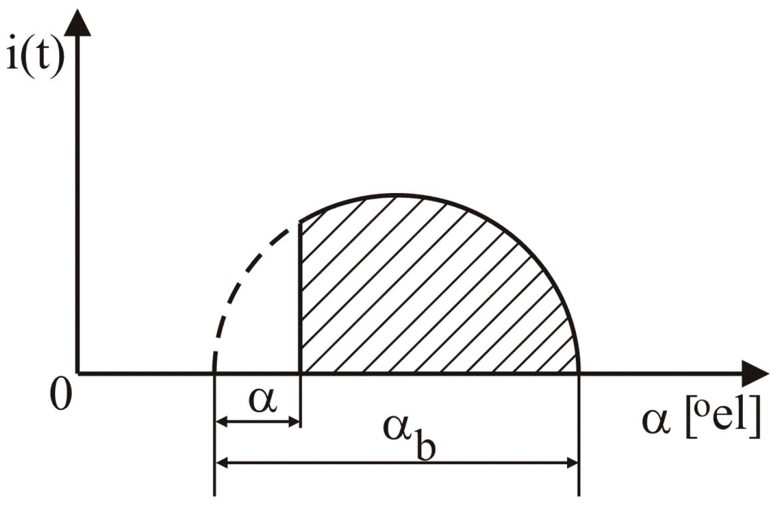
It can be noticed in the above formula that the conduction current starts at the firing angle α, and stops at the locking angle α_b, as shown in Figure 1.

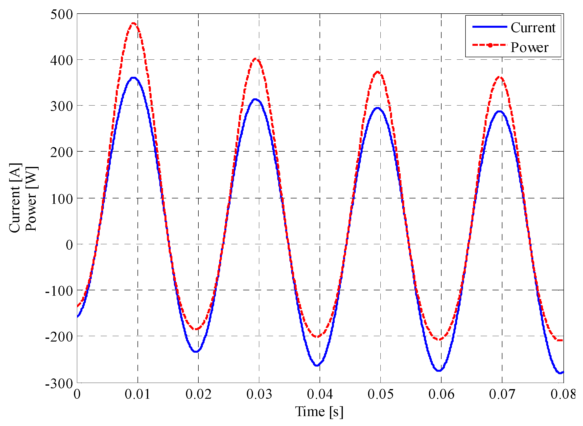
Taking into account Equation (3) of the current evolution and the initial Equation (1), the next diagram, Figure 2, represents the time variation of both power loss p(t) and the electrical current i(t).

By solving the above integral expression, the RMS current value results, given by the next relation:

$$I_{RMS}=I_m{\left(\frac{1}{2\pi }\left\{\begin{array}{l}\frac{{\alpha }_b-\alpha }{2}-\frac{1}{2}\sin \left({\alpha }_b-\alpha \right)\cos \left({\alpha }_b+\alpha -2\phi \right)+\frac{2\sin \left(\alpha -\phi \right)\frac{\omega L}{R}}{1+{\left(\frac{\omega L}{R}\right)}^2}\left[\begin{array}{l}\left(\begin{array}{l}\sin \left({\alpha }_b-\phi \right)+\\ +\frac{\omega L}{R}\cos \left({\alpha }_b-\phi \right)\end{array}\right)e^{-\frac{{\alpha }_b-\alpha }{\omega L/R}}-\\ -\sin \left(\alpha -\phi \right)-\frac{\omega L}{R}\cos \left(\alpha -\phi \right)\end{array}\right]-\\ -\frac{\omega L}{2R}{\sin }^2\left(\alpha -\phi \right)\left(e^{-2\frac{{\alpha }_b-\alpha }{\omega L/R}}-1\right)\end{array}\right\}\right)}^{\frac{1}{2}}$$

(5)

The average current from the Equation (3), has the expression below,

$$I_{TAV}=\frac{1}{2\pi }{\displaystyle \underset{\alpha }{\overset{{\alpha }_b}{\int }}i\left(t\right)d\left(\omega t\right)}=\frac{I_m}{2\pi }{\displaystyle \underset{\alpha }{\overset{{\alpha }_b}{\int }}\left[\sin \left(\omega t-\phi \right)-\sin \left(\alpha -\phi \right)e^{-\frac{\omega t-\alpha }{\omega L/R}}\right]}d\left(\omega t\right)=I_m\frac{\cos \alpha -\cos {\alpha }_b}{2\pi \cos \phi }$$

(6)

In the case of the resistive load, when the ratio $\frac{\omega L}{R}\to 0\hspace{0.17em};\hspace{0.17em}tg\phi \to 0$, the above expressions of the RMS current become:

$$I_{RMS}=\frac{I_m}{2}\sqrt{\frac{1}{\pi }\left({\alpha }_b-\alpha \right)-\frac{1}{2\pi }\left(\sin 2{\alpha }_b-\sin 2\alpha \right)}$$

(7)

and for the average current,

$$I_{TAV}=I_m\frac{\cos \alpha -\cos {\alpha }_b}{2\pi }.$$

(8)

Using the power loss Equation (2) for power semiconductors and the relations shown by Equations (5) and (6), the formula to calculate the power loss through the semiconductor device in the case of a RL load is provided as:

$$P_{sRL}=V_T{I}_m\frac{\cos \alpha -\cos {\alpha }_b}{2\pi \cos \phi }+r_T\frac{I_m^2}{2\pi }\left\{\begin{array}{l}\frac{{\alpha }_b-\alpha }{2}-\frac{1}{2}\sin \left({\alpha }_b-\alpha \right)\cos \left({\alpha }_b+\alpha -2\phi \right)+\\ \frac{2\sin \left(\alpha -\phi \right)\frac{\omega L}{R}}{1+{\left(\frac{\omega L}{R}\right)}^2}\left[\begin{array}{l}\left(\begin{array}{l}\sin \left({\alpha }_b-\phi \right)+\\ +\frac{\omega L}{R}\cos \left({\alpha }_b-\phi \right)\end{array}\right)e^{-\frac{{\alpha }_b-\alpha }{\omega L/R}}\\ -\sin \left(\alpha -\phi \right)-\frac{\omega L}{R}\cos \left(\alpha -\phi \right)\end{array}\right]\\ -\frac{\omega L}{2R}{\sin }^2\left(\alpha -\phi \right)\left(e^{-2\frac{{\alpha }_b-\alpha }{\omega L/R}}-1\right)\end{array}\right\}$$

(9)

In the case of the resistive load, the above expression becomes,

$$P_{sR}=V_T{I}_m\frac{\cos \alpha -\cos {\alpha }_b}{2\pi c}+r_T\frac{I_m^2}{4\pi }\left[\left({\alpha }_b-\alpha \right)-\frac{1}{2}\left(\sin 2{\alpha }_b-\sin 2\alpha \right)\right]$$

(10)

The foregoing expressions of power losses, together with the values of junction-case, case-heatsink, and heatsink-environment thermal resistance of the power semiconductor, can be used to compute the junction temperature and case temperature. Hence, the expression for the junction temperature is:

$${\theta }_j={\theta }_a+\left(R_{thjc}+R_{thck}+R_{thka}\right)P_{sRL}$$

(11)

The case temperature of the power semiconductor can be computed with the following relation,

$${\theta }_c={\theta }_a+\left(R_{thck}+R_{thka}\right)P_{sRL}.$$

(12)

Generally, the junction-case and the heatsink-environment thermal junctions are not constant values. Thus, the junction-case thermal resistance depends on the current waveform (rectangular or sinusoidal) and the conduction angle from the respective current waveform. Depending on the type of power semiconductor, the variation of the junction-case thermal resistance against conduction angle are presented in the datasheets. Also, the heatsink-environment thermal junction depends on the type of the heatsink and cooling method: natural or forced. In the heatsink datasheets there are graphics with the variation of the heatsink-environment thermal junction against air speed. Moreover, the case-heatsink thermal resistance depends on the type of the power semiconductor case and the cooling method. Its value is specified in the power semiconductor device datasheets.

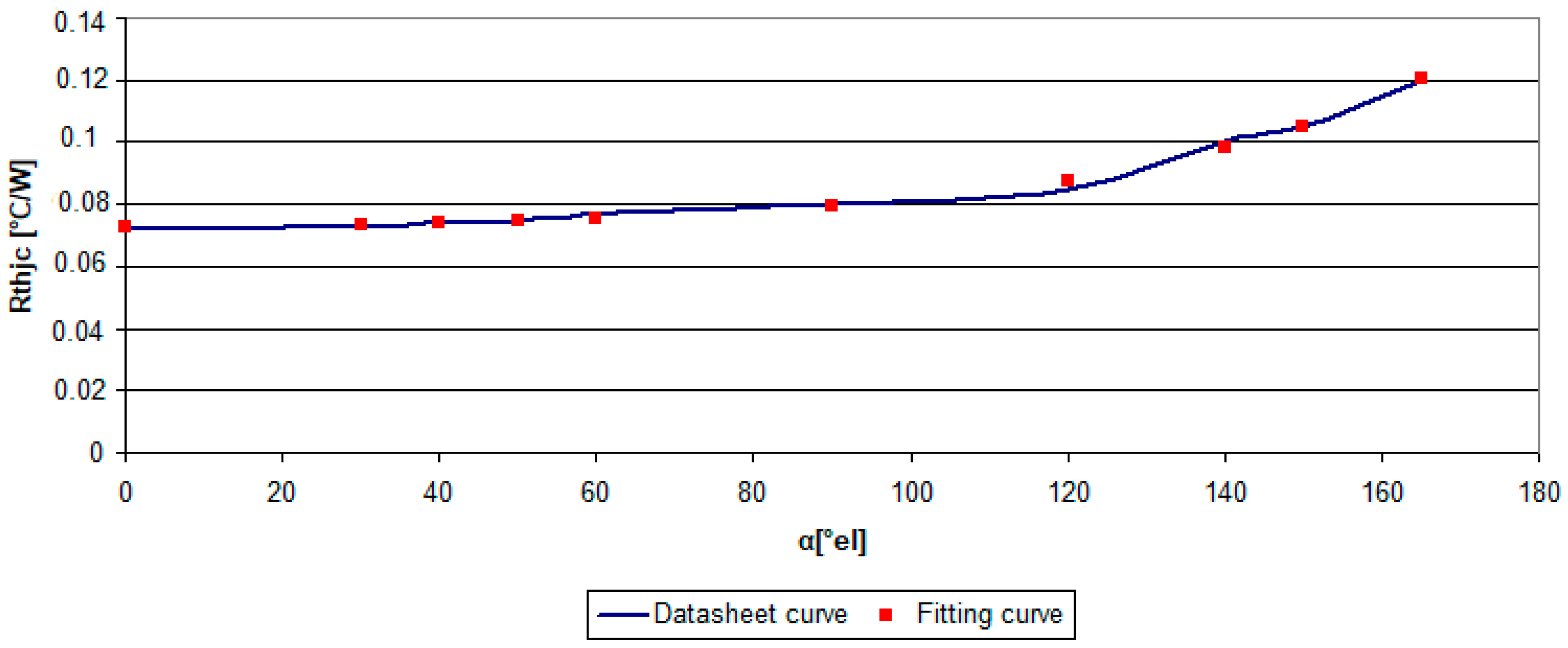
In the following, the SKT 340 thyristor made by Semikron company, will be analyzed in order to obtain an analytical expression to study the heating aspects during steady-state conditions. From the datasheets the following data can be obtained: V_T = 1 V; r_T = 0.9 mΩ; R_thck = 0.02 °C/W in the case of double side cooling. With the aim to get the analytical expression to compute the junction and case temperature, the variation curve of junction-case thermal resistance against conduction angle from the datasheet, has been approximated with its fitting curve, Figure 3, which has the mathematical expression,

$$R_{thjc}=a_1+b_1{e}^{-\frac{\alpha }{c_1}}$$

(13)

where the parameters a₁, b_1, and c₁ have the following values: a₁ = 0.0718; b₁ = 0.00082, and c₁ = −40.584. The relative error according to the Equation (13) is less than ±1.2%.

It can be observed that the initial datasheet curve, junction-case thermal resistance against conduction angle, has been transformed into the variation of the junction-case thermal resistance against firing angle (firing angle = locking angle − conduction angle) because the computing expressions of power loss depend on the firing angle and not on the conduction angle.

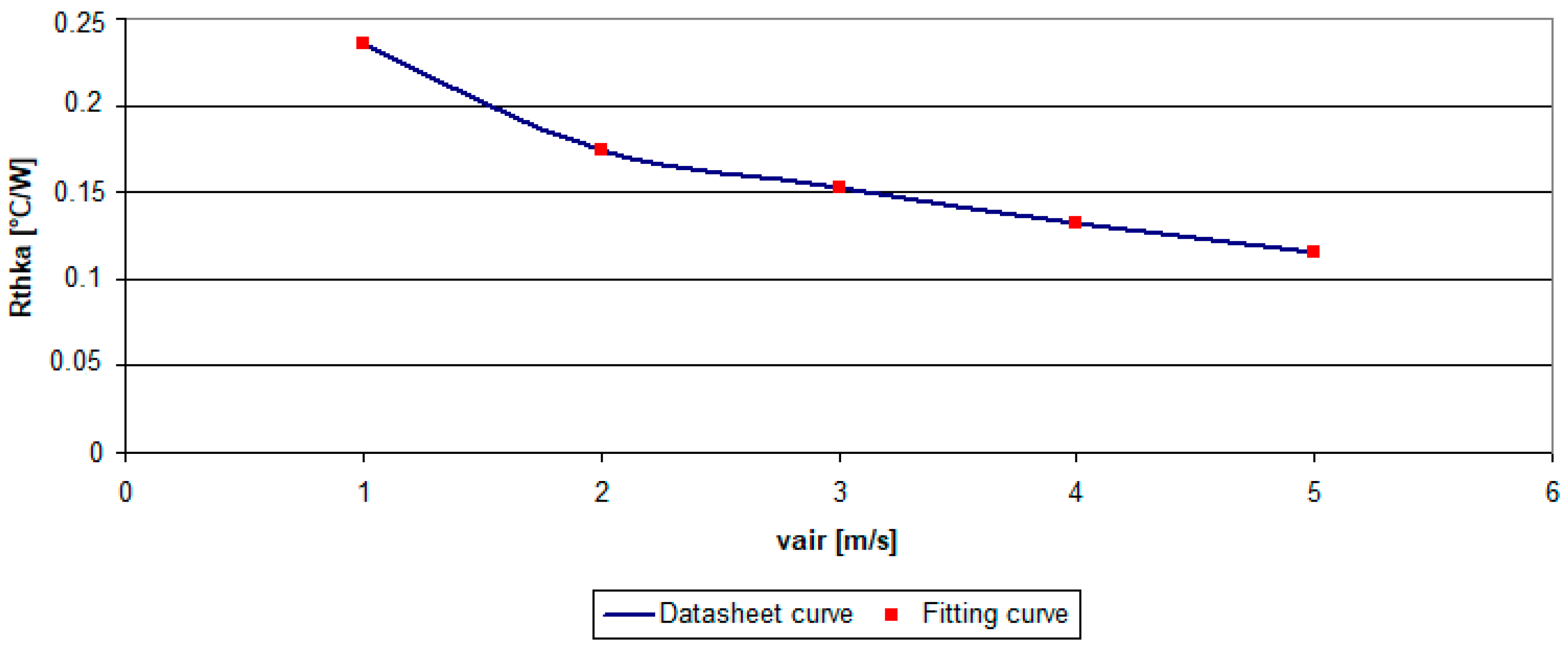
The cooling of the SKT 340 thyristor is obtained through the aluminum heatsink type R150-E50 made by IPRS Baneasa company. The variation curve of heatsink-environment thermal resistance against air speed in the case of forced cooling, from the datasheet, has been approximated with its fitting curve, Figure 4, which has the mathematical expression,

$$R_{thka}=a_2+b_2{v}_{air}^2+c_2{v}_{air}^2\ln v_{air}+d_2\frac{\ln v_{air}}{v_{air}^2}$$

(14)

where the parameters a₂, b₂, c₂, and d₂ have the following values: a₂ = 0.25; b₂ = −0.0153, and c₂ = 0.0064 and d₂ = −0.1899. The relative error according to Equation (14) is less than ±0.03%. In the case of forced cooling, decreasing of the heatsink-environment thermal resistance when the air speed is increasing can be noticed. Thus, the junction temperature of the tyristor can be computed with the formula,

$${\theta }_j={\theta }_a+\left(a_1+b_1{e}^{-\frac{\alpha }{c_1}}+R_{thck}+a_2+b_2{v}_{air}^2+c_2{v}_{air}^2\ln v_{air}+d_2\frac{\ln v_{air}}{v_{air}^2}\right)P_{sRL}$$

(15)

and the case temperature of the same power semiconductor will be calculated with,

$${\theta }_c={\theta }_a+\left(R_{thck}+a_2+b_2{v}_{air}^2+c_2{v}_{air}^2\ln v_{air}+d_2\frac{\ln v_{air}}{v_{air}^2}\right)P_{sRL}$$

(16)

Taking into account the expression of power loss (9) in a general case of a resistive-inductive load, the next final relations are obtained to compute the junction temperature,

$$\begin{array}{l}{\theta }_j={\theta }_a+V_T{I}_m\frac{\cos \alpha -\cos {\alpha }_b}{2\pi \cos \phi }\left(a_1+b_1{e}^{-\frac{\alpha }{c_1}}+R_{thck}+a_2+b_2{v}_{air}^2+c_2{v}_{air}^2\ln v_{air}+d_2\frac{\ln v_{air}}{v_{air}^2}\right)+\\ +r_T\frac{I_m^2}{2\pi }\left(a_1+b_1{e}^{-\frac{\alpha }{c_1}}+R_{thck}+a_2+b_2{v}_{air}^2+c_2{v}_{air}^2\ln v_{air}+d_2\frac{\ln v_{air}}{v_{air}^2}\right)\left\{\begin{array}{l}\frac{{\alpha }_b-\alpha }{2}-\frac{1}{2}\sin \left({\alpha }_b-\alpha \right)\cos \left({\alpha }_b+\alpha -2\phi \right)+\\ \frac{2\sin \left(\alpha -\phi \right)\frac{\omega L}{R}}{1+{\left(\frac{\omega L}{R}\right)}^2}\left[\begin{array}{l}\left(\begin{array}{l}\sin \left({\alpha }_b-\phi \right)+\\ +\frac{\omega L}{R}\cos \left({\alpha }_b-\phi \right)\end{array}\right)e^{-\frac{{\alpha }_b-\alpha }{\omega L/R}}\\ -\sin \left(\alpha -\phi \right)-\frac{\omega L}{R}\cos \left(\alpha -\phi \right)\end{array}\right]\\ -\frac{\omega L}{2R}{\sin }^2\left(\alpha -\phi \right)\left(e^{-2\frac{{\alpha }_b-\alpha }{\omega L/R}}-1\right)\end{array}\right\}\end{array}$$

(17)

and the case temperature of the tyristor,

$$\begin{array}{l}{\theta }_c={\theta }_a+V_T{I}_m\frac{\cos \alpha -\cos {\alpha }_b}{2\pi \cos \phi }\left(R_{thck}+a_2+b_2{v}_{air}^2+c_2{v}_{air}^2\ln v_{air}+d_2\frac{\ln v_{air}}{v_{air}^2}\right)+\\ +r_T\frac{I_m^2}{2\pi }\left(R_{thck}+a_2+b_2{v}_{air}^2+c_2{v}_{air}^2\ln v_{air}+d_2\frac{\ln v_{air}}{v_{air}^2}\right)\left\{\begin{array}{l}\frac{{\alpha }_b-\alpha }{2}-\frac{1}{2}\sin \left({\alpha }_b-\alpha \right)\cos \left({\alpha }_b+\alpha -2\phi \right)+\\ \frac{2\sin \left(\alpha -\phi \right)\frac{\omega L}{R}}{1+{\left(\frac{\omega L}{R}\right)}^2}\left[\begin{array}{l}\left(\begin{array}{l}\sin \left({\alpha }_b-\phi \right)+\\ +\frac{\omega L}{R}\cos \left({\alpha }_b-\phi \right)\end{array}\right)e^{-\frac{{\alpha }_b-\alpha }{\omega L/R}}\\ -\sin \left(\alpha -\phi \right)-\frac{\omega L}{R}\cos \left(\alpha -\phi \right)\end{array}\right]\\ -\frac{\omega L}{2R}{\sin }^2\left(\alpha -\phi \right)\left(e^{-2\frac{{\alpha }_b-\alpha }{\omega L/R}}-1\right)\end{array}\right\}\end{array}$$

(18)

It can be noticed that both the junction and case temperature of the tyristor depend on the firing angle, conduction current, air speed in the case of forced cooling, and the values of the resistive–inductive load.

3. Three-Dimensional Thermal Model

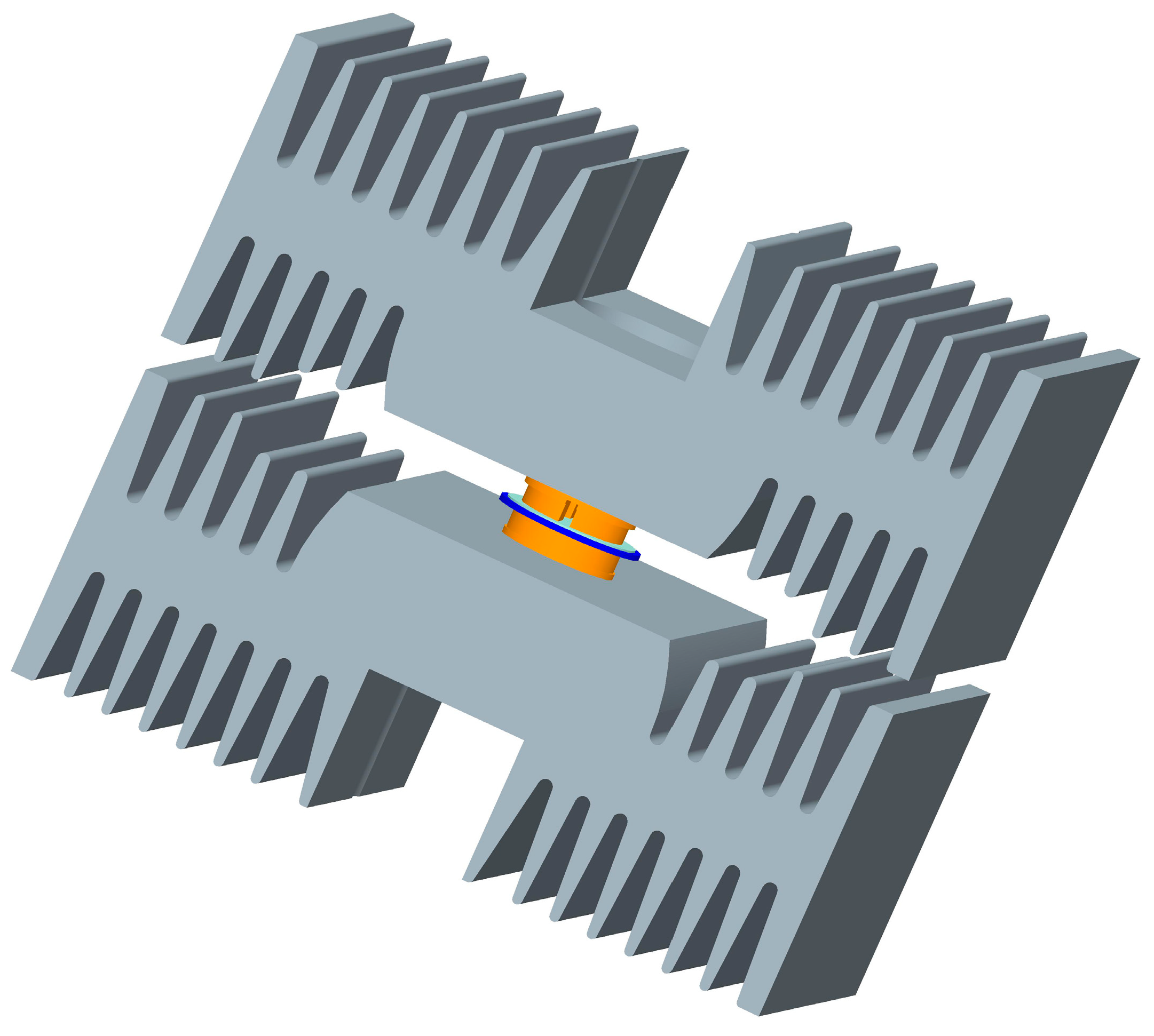
A power assembly made from the tyristor type SKT 340 mounted between a heatsink type R150-E50 made from aluminium has been studied. This power assembly can be considered as the main component part of a power bidirectional rectifier which provides DC power supply for a resistive-inductive load. The average direct current which flows through the tyristor has been assumed to be 250 A. Because the internal resistance value is 0.9 mΩ, it results in the power loss related to the analyzed thyristor to be about 56.25 W.

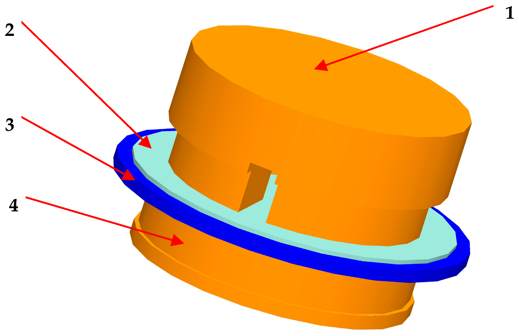
The three-dimensional geometry of the above described power assembly, has been performed using the software package Pro-ENGINEER. The 3D thermal model of the tyristor includes all the component parts which are directly involved in the thermal exchange between components and from the elements to the environment: anode copper pole, molybdenum disc, silicon chip and cathode copper pole, as shown in Figure 5. Hence, the extreme components: the anode and the cathode pole, both made from copper, can be observed. The cathode has in the upper middle part, a channel where the gate is mounted. Between these main components, there is placed the molybdenum disc having a larger diameter than the silicon chip.

The ceramic enclosure of the power semiconductor device has not been included in the 3D model since the total heat flowing through it is less important than the heat flowing through the copper poles. The mechanical elements which are not important for the heat transfer within the power semiconductor and from the power device to the environment (e.g., the centering hole on the poles) have been removed. The material properties of every component part of the power semiconductor and the heatsink are described in the

Table 1. Material data.

Parameter	Material
	Copper	Silicon	Molybdenum	Aluminium
γ (kg/m3)	8900	2330	10,220	2700
c (J/kg°C)	387	702	255	900
λ (W/m°C)	385	124	138	200

and the 3D thermal model of the thyristor together with its heatsinks for double side cooling are shown in Figure 6.

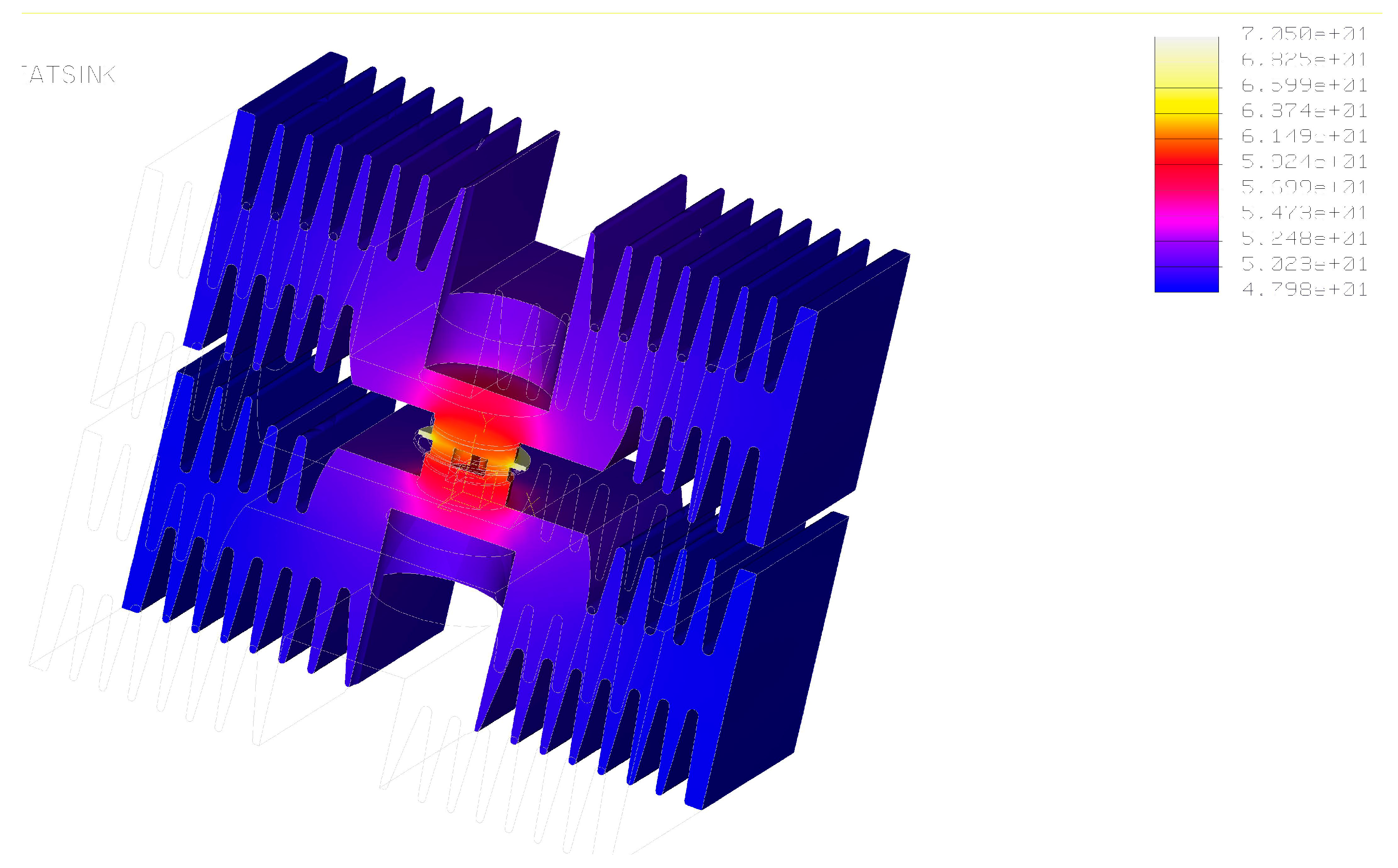
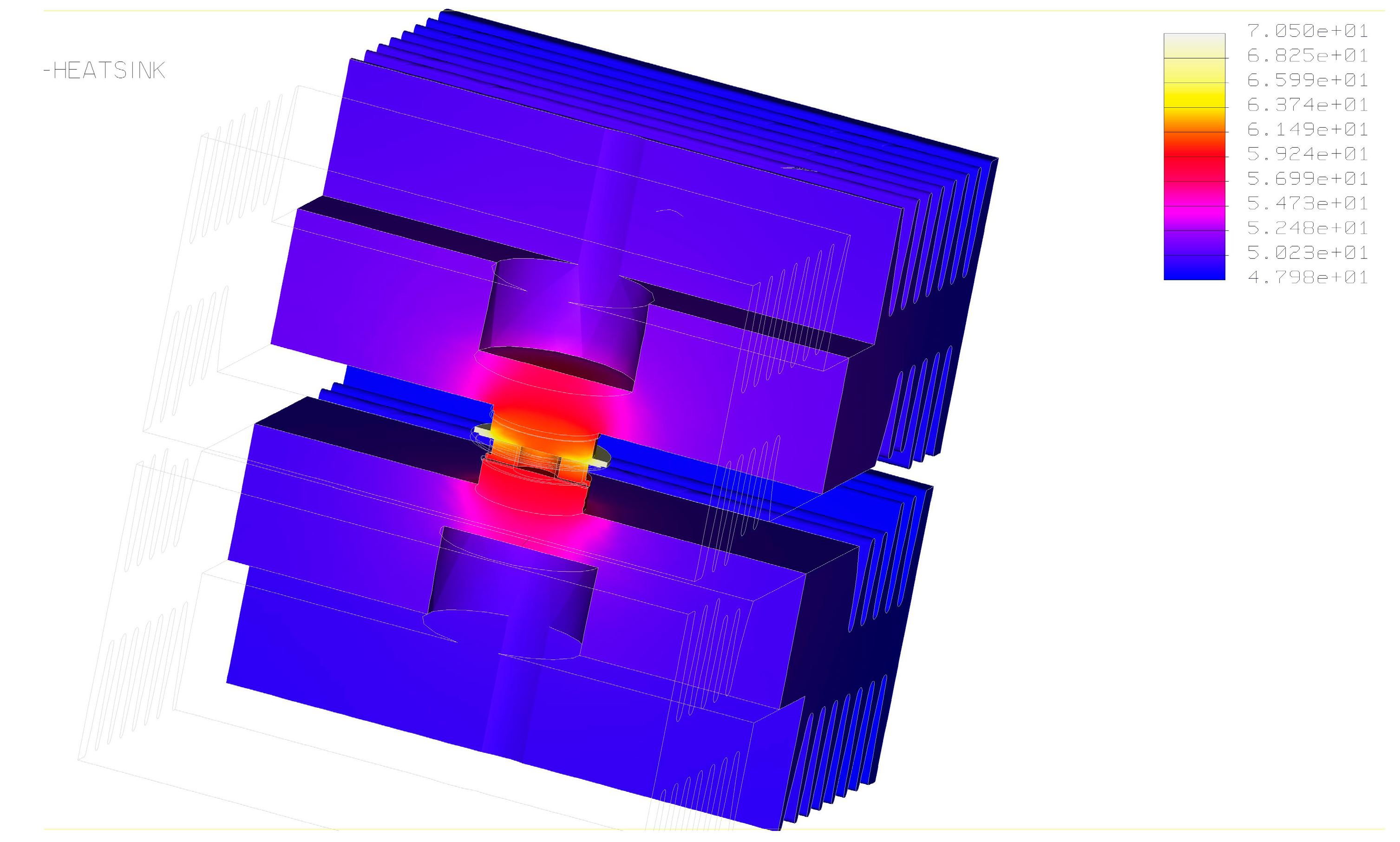
In order to perform the thermal simulations during steady-state conditions, the dedicated Pro-MECHANICA software package based on the finite element method has been used. The heat load, actually the power loss, has been applied on the active surface of the silicon chip of the thyristor. A uniform spatial distribution on this surface was considered. The ambient temperature was about 20 °C. From experimental tests, a convection coefficient value of 14.45 W/m²·°C was calculated for this type of heatsink considering forced cooling with an air speed of 3 m/s.

The convection condition has been considered as a boundary condition for the outer boundaries, as heatsinks. The convection coefficient has been applied on outer surfaces of heatsinks with a uniform spatial variation and a bulk temperature of 20 °C. The mesh of the 3D power assembly thermal model (thyristor between heatsinks) has been done using tetrahedral solid elements, and the single pass adaptive convergence method was considered in order to solve the thermal steady-state simulations. Further, some thermal simulations during steady-state conditions, have been performed, as shown in Figure 7 and Figure 8.

The temperature distribution of the tyristor which uses double cooling, both on anode and cathode, in the case of air speed value of 3 m/s, firing angle equal with 50 °el, direct current of 250 A, load resistance by 3 Ω and the load inductance about 30 mH, is shown in the above pictures, Figure 7 and Figure 8. A maximum temperature of the power semiconductor can be noticed on the silicon surface and is about 70.49 °C, and a minimum temperature of 47.97 °C, on the heatsink outer surfaces.

4. Discussion of the Results

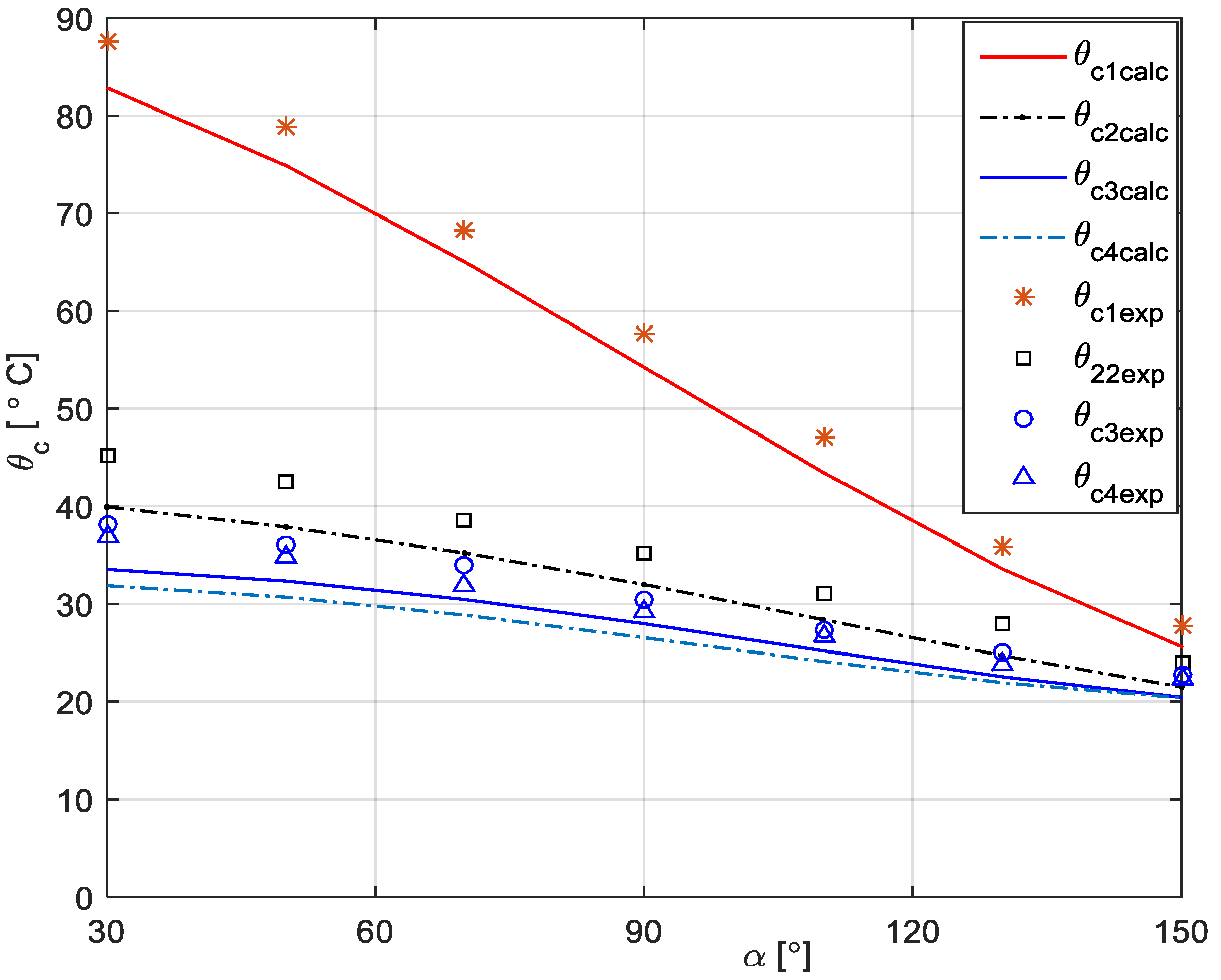
Taking into account the solutions for the equation of junction temperature (17) and case temperature (18), it can be analyzed the influence of air speed, electrical current, load resistance and load inductance on the tyristor heating. Further on, the thermal analysis refers to the junction and case temperature of the power semiconductor.

The variation of the junction and case temperature of the tyristor type SKT 340 against firing angle at different air speed values of 1, 3, and 6 m/s in the case of forced cooling, is depicted in the Figure 9, and respectively, Figure 10. A decreasing of the of the junction and case temperature is to be observed when the firing angle increases. This is explained because when the firing angle increases, actually, the conduction angle decreases (condution angle = locking angle − firing angle = π − firing angle), thus, the tyristor will be passed by a less conductive current and, as a consequence, the power loss decreases, so, the junction and case temperature will decrease. Also, when the air speed increases, the junction and case temperature decrease because of better cooling of the power assembly. A maximum junction temperature of 102 °C can be observed when the firing angle is 30 °el, in the case of air speed about 1 m/s, upper curve in Figure 9, and a minimum of junction temperature of 24.85 °C when the firing angle is 150 °el, in the case of air speed being about 6 m/s, the lower curve.

The maximum case temperature is 78.81 °C when the firing angle is 30°el and the air speed is about 1 m/s, as shown in Figure 10 (upper curve), and the minimum case temperature is about 22.6 °C when the firing angle is 150 °el for an air speed of 6 m/s (lower curve). It can be noticed that the simulation values for the junction temperature, are lower than the calculated ones. This can be explained because during calculation of the formula, concentrated parameters have been considered, as thermal load, but actually, the thermal load is distributed on the surface of the silicon chip, so the thermal conduction and convection surfaces allow a better heat transfer from the silicon chip to the environment. Thus, the maximum simulated junction temperature is 98.2 °C when the firing angle is 30 °el and the air speed is about 1 m/s, as shown in Figure 9, and the minimum maximum simulated junction temperature is 22.6 °C when the firing angle is 150 °el for an air speed about 6 m/s.

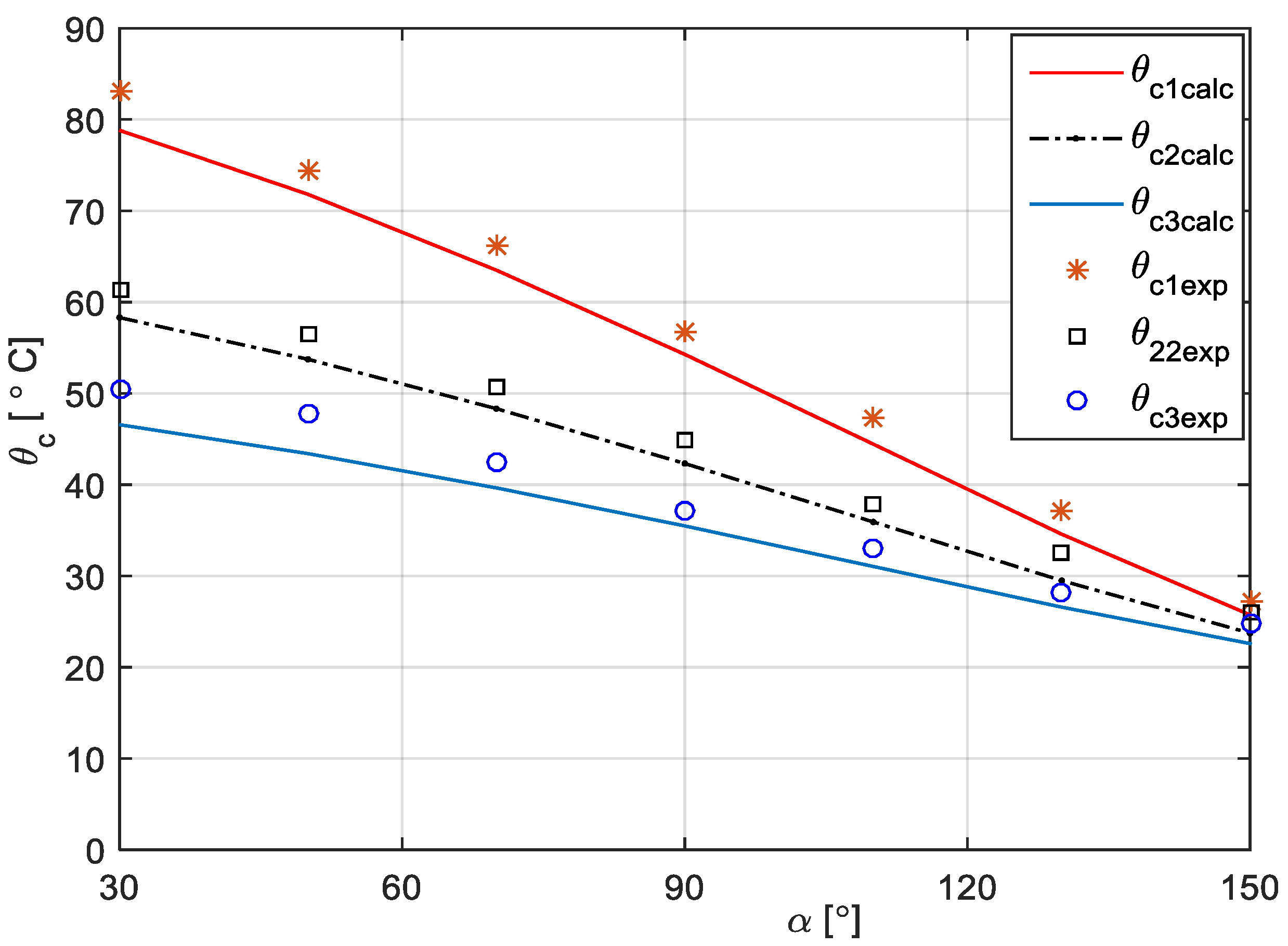
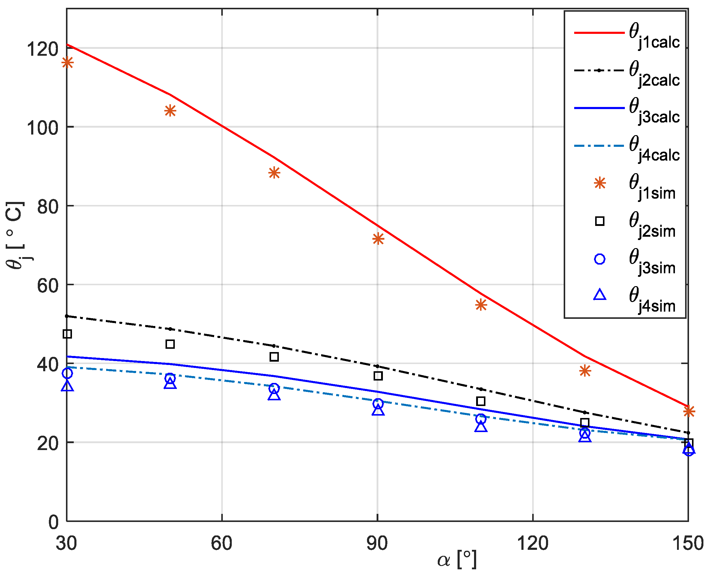
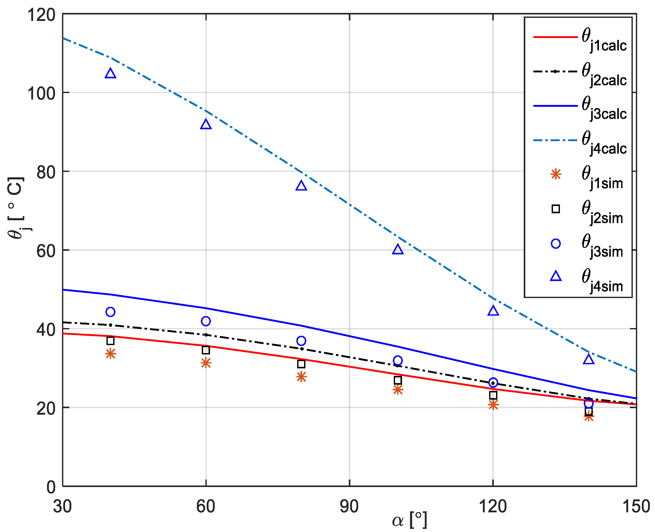
The junction and case temperature variation against the firing angle for different conduction current values of 200, 250, 300, and 340 A for an air speed of about 3 m/s, a resistive load of 3 Ω, and inductance load of 30 mH, as is presented in Figure 11 and Figure 12, respectively. The same decreasing variation of both junction and case temperature against firing angle can be observed, as with larger values of the temperatures when the conduction current increases. This is explained because of higher values of the power loss when the conduction current is increasing. Thus, the maximum junction temperature of 104.3 °C when the firing angle is 30 °el, in the case of conduction current about 340 A, Figure 11 (top curve), and a minimum of junction temperature of 24.52 °C when the firing angle is 150 °el and the conduction current is 200 A (bottom curve). The maximum case temperature is 72.5 °C when the firing angle is 30 °el and the conduction current is 340 A, as in Figure 12 (top curve), and the minimum case temperature is about 22.82 °C when the firing angle is 150 °el and the conduction current is 200 A (bottom curve). As in the previously analyzed situation, for different air speeds and with the same explanation, the simulated junction temperatures are lower than the calculated ones. Hence, the maximum simulated junction temperature is 99.8 °C when the firing angle is 30 °el and the conduction current is 340 A, as in Figure 11, and the minimum maximum simulated junction temperature is 22.4 °C when the firing angle is 150 °el and the current is about 200 A.

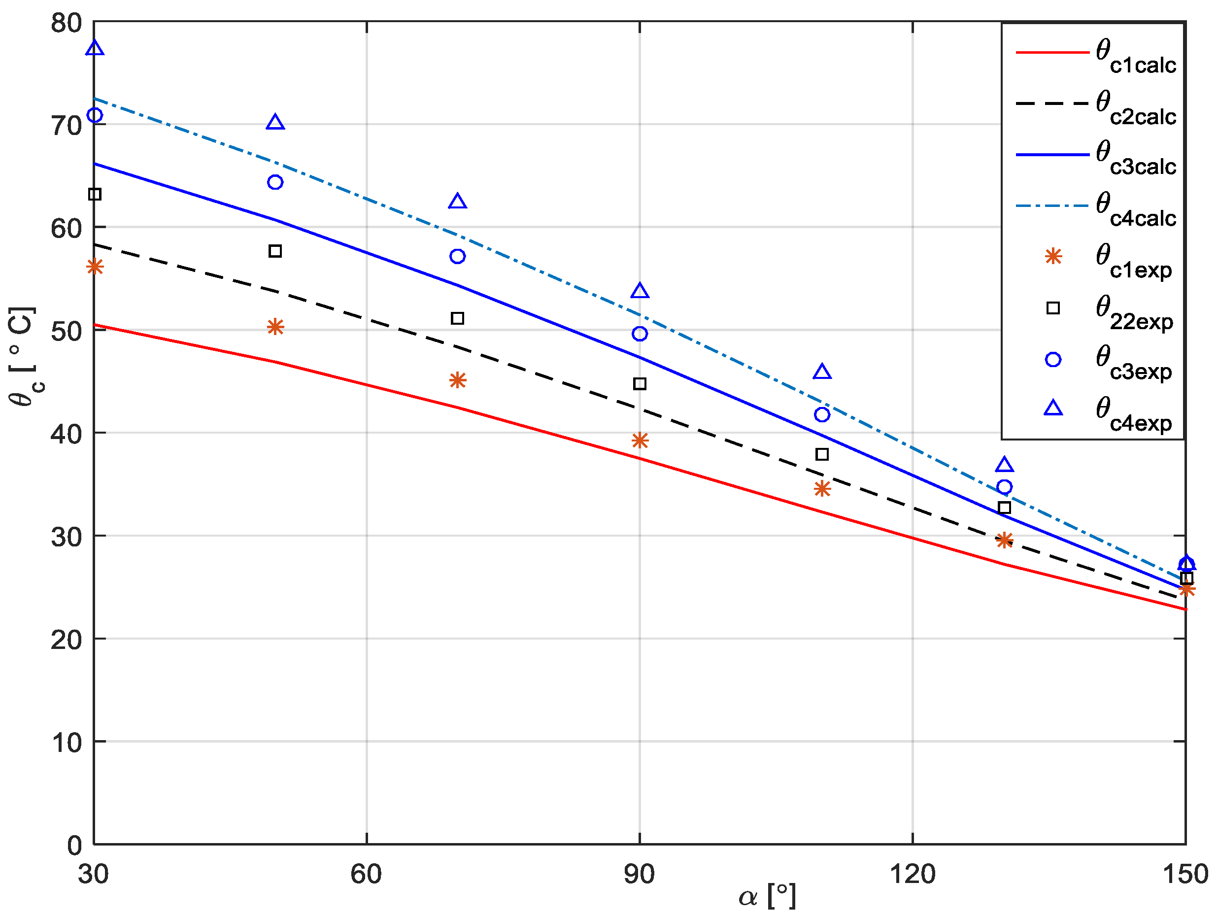
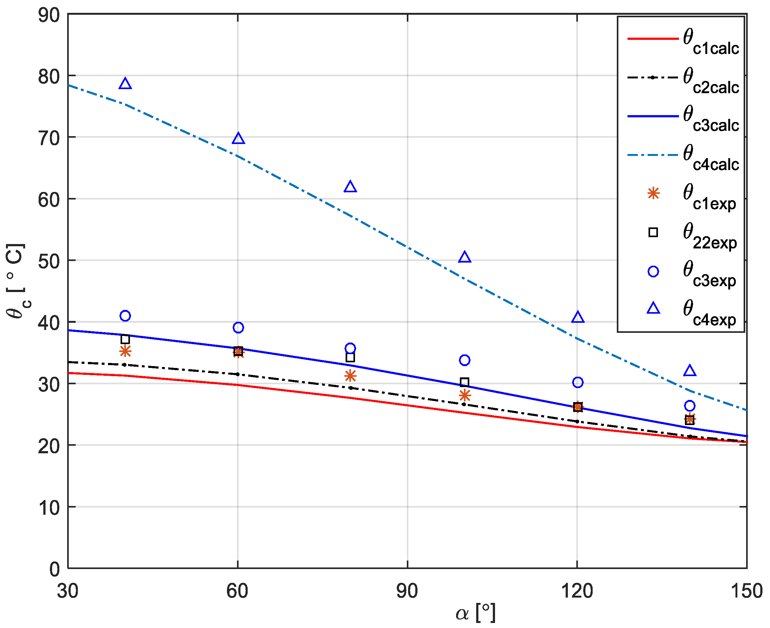
The variation of the junction and case temperature against firing angle for different resistive load values of 1.4, 5, 10, and 16 Ω when the air speed was about 3 m/s, the conduction current is 200 A, and an inductive load of 30 mH, as described in Figure 13 and Figure 14, respectively. The bottom curve corresponds to a resistance value of 16 Ω, and the top curve has been drawn for a resistance value of 1.4 Ω. It is to observed that for higher resistance values, both junction and case temperatures decrease.

This is explained because at higher values of load resistance, the load current will decrease, and also the power loss of the tyristor, so the junction and case temperatures will have lower values. For instance, in the case of firing angle being about 90 °el, the junction temperature is about 74.8 °C in the case of load resistance of 1.4 Ω, as in Figure 13, and the temperature value is 30.5 °C when the resistance becomes 16 Ω. Also, at the same firing angle of 90 °el, the case temperature is 54.23 °C when the load resistance of 1.4 Ω, as in Figure 14 (top curve), and the temperature value is 26.54 °C for a resistance of 16 Ω (bottom curve). With the same explanation as in previously analyzed situations, at different air speeds and currents, the simulated junction temperatures are lower than the calculated ones. Thus, for instance, when the firing angle is about 50 °el, the simulated junction temperature value of 104.1 °C is lower than the calculated one of 108.12 °C in the case of load resistance of 1.4 Ω, as in Figure 13, and the simulated junction temperature value of 34.5 °C is lower than the calculated one of 37.17 °C at the resistance value of 16 Ω.

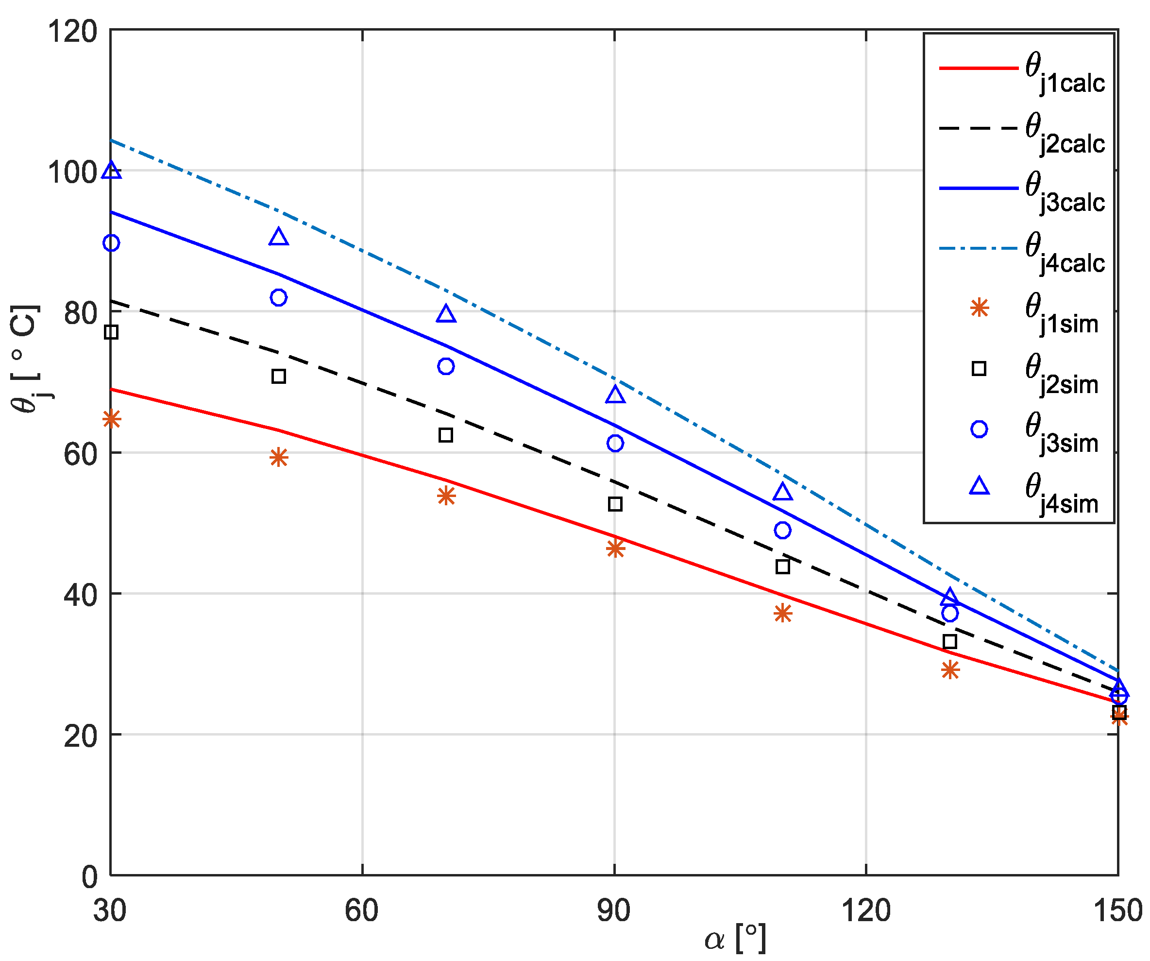
The junction and case temperature variation against firing angle for different inductive load values of 18, 30, 55, and 200 mH when the air speed is about 3 m/s, the conduction current is 200 A, and the resistive load of 10 Ω, is presented in Figure 15 and Figure 16, respectively. The bottom curve corresponds to an inductance value of 18 mH, and the top curve has been drawn for an inductance value of 200 mH. It can be observed that when the inductance increases, the junction and case temperatures also increase. This is explained because at higher value of the inductance, a dominant inductive load, actually the power rectifier, becomes a current generator, so the power loss within the tyristor will increase, and finally, the junction and case temperature increases. For instance, when the firing angle is 60 °el, the junction temperature is about 95.28 °C in the case of load inductance of 200 mH, Figure 15 (top mark), and the temperature value is 35.65 °C when the inductance becomes 18 mH (bottom mark). For the same firing angle of 60 °el, the case temperature is 66.89 °C when the load inductance is 200 mH, as in Figure 16, and the temperature value is 29.74 °C for an inductance of 18 mH. As in the previously analyzed situations, the simulated junction temperatures are lower than the calculated ones. For instance, when the firing angle is about 60 °el, the simulated junction temperature value of 91.6 °C is lower than the calculated one of 95.28 °C in the case of load inductance of 200 mH, as in Figure 15, and the simulated junction temperature value of 31.3 °C is lower than the calculated one of 35.65 °C at the resistance value of 18 mH.

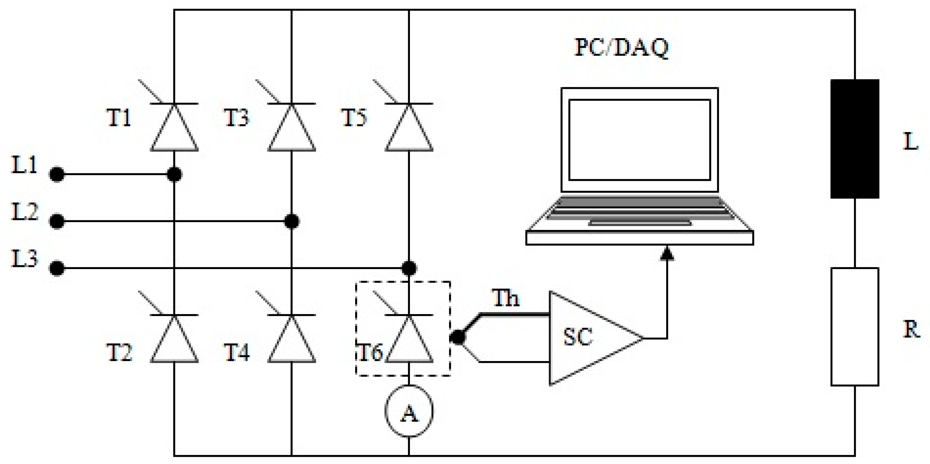
In order to validate the mathematical models presented above, some experimental tests have been performed with the aim to obtain the case temperature value of the thyristor. The temperatures have been acquired using type K thermocouples. A drawing of the device under test with the current and temperature measurement system is presented in the Figure 17. The three-phase full bridge rectifier made with the tyristors T1–T6, is supplied from the main grid with the terminals L1, L2, and L3. In series with the thyristor T6, actually the device under test, mounted to the ammeter A, to measure the current value. In this case, thyristor T6 is placed at the thermocouple Th in order to get the temperature data.

The thermocouple provides a low magnitude voltage signal that needs to be amplified by a signal conditioning board SC, type AT2F-16 with the error of ±0.5%. The amplified voltage signal is used as input data for a data acquisition board type PC-LPM-16. This can be programmed using the LabVIEW software package. The sampling rate was 50 kS/s and the analogue inputs have a resolution on 12 bits. The three-phase power rectifier supplies the resistive-inductive load RL.

In the case of temperature variation against firing angle for different air speed values, shown in Figure 10, the maximum case temperature is about 83.1 °C when the air speed is 1 m/s and the firing angle is 30 °el, and the minimum case temperature is 24.8 °C for a firing angle of 150 °el and the air speed of 6 m/s. It can to observed that the experimental values are higher than the calculated ones because, in fact, the semiconductor case does not cool evenly. Actually, due to the mounting technology of the power assembly (thyristor case between heatsinks of rather large sizes), the airflow does not cool the surface of the semiconductor case quite well. So, for instance at the firing angle of 90 °el, the experimental case temperature is 56.8 °C higher than the computed temperature of 54.2 °C for an air speed of 1 m/s, and there is also an experimental case temperature of 37.2 °C which is higher than the computed one of 35.48 °C for an air speed of 6 m/s.

The thermal analysis against firing angle for different conduction current values, shown in Figure 12, outlines the same higher experimental values as the calculated ones. Thus, in the case of a 90 °el firing angle, the experimental case temperature is 53.6 °C, which is higher than the computed temperature of 51.45 °C when the conduction current is 340 A, and there is also an experimental case temperature of 39.2 °C higher than the calculated case temperature of 37.49 °C at the conduction current of 200 A.

Also, in the case of load resistance or load inductance variation, the experimental case temperatures are higher than the computed ones. For instance, when the load resistance has the value of 1.4 Ω and the firing angle is 30 °el, the experimental case temperature of 87.6 °C is higher than the computed ones of 82.84 °C, as in Figure 14. On the other hand, for an inductive load of 200 mH and a firing angle of 60 °el, the experimental case temperature of 69.6 °C is higher than the calculated one of 66.89 °C, shown in Figure 16.

Certainly, there are different temperature values resultant from experimental tests with respect to calculations because of measurement errors, thermal model simplifications, and mounting test conditions. However, the difference between experimental and calculation results is less than 5 °C.

5. Conclusions

In order to understand and optimize the operating mechanisms of power converters, the thermal behaviour of the power electronic device itself is of real importance. The simulation of the thermal processes of the power semiconductor junction, which depends on the power device design, may lead to new functions regarding the optimization of power semiconductor converters. This has an important impact on the development and test costs of new power converters.

Extending the thermal models to specific applications allows the user of power devices to choose the right ratings, to evaluate critical load cycles, and to identify potential overload capacities for dynamic operating conditions. The described thermal model has an important potential for different applications, including:

• development support;
• to identify user risks;
• to evaluate the right rated current;
• to evaluate overload capacity without destructive failure of the power device.

This paper describes a mathematical model related to the junction and case temperature of a thyristor from a power rectifier. The thermal model allows for the calculation of the junction and case temperature in the situation of conduction current variation, load type variation, and air speed in the case of forced cooling. Having the possibility of 3D thermal modelling and simulation, it will improve the power assembly design and provide new solutions for a better cooling of the power semiconductors and power converter design.

The experimental tests validated the proposed mathematical model. There are close values between experimental, simulation, and computing of junction and case temperature.