Article

A General Parameter Identification Procedure Used for the Comparative Study of Supercapacitors Models

Power Electronics Systems Group; Universidad Carlos III de Madrid, 28911 Leganés, Spain
*
Author to whom correspondence should be addressed.
Energies 2019, 12(9), 1776; https://doi.org/10.3390/en12091776
Submission received: 22 March 2019 / Revised: 3 May 2019 / Accepted: 7 May 2019 / Published: 10 May 2019
(This article belongs to the Special Issue Energy Storage and Management for Electric Vehicles)

Abstract

:
Supercapacitors with characteristics such as high power density, long cycling life, fast charge, and discharge response are used in different applications like hybrid and electric vehicles, grid integration of renewable energies, or medical equipment. The parametric identification and the supercapacitor model selection are two complex processes, which have a critical impact on the system design process. This paper shows a comparison of the six commonly used supercapacitor models, as well as a general and straightforward identification parameter procedure based on Simulink or Simscape and the Optimization Toolbox of Matlab®. The proposed procedure allows for estimating the different parameters of every model using a different identification current profile. Once the parameters have been obtained, the performance of each supercapacitor model is evaluated through two current profiles applied to hybrid electric vehicles, the urban driving cycle (ECE-15 or UDC) and the hybrid pulse power characterization (HPPC). The experimental results show that the model accuracy depends on the identification profile, as well as the robustness of each supercapacitor model. Finally, some model and identification current profile recommendations are detailed.

1. Introduction

Energy storage systems are essential in the industrial, medical, renewable or transportation sectors, as well as other sectors. Some characteristics like high power density, reliability and safety are critical in those sectors, this is why the electrochemical double layer capacitor or the supercapacitor play an important role [1].
Many application areas in which supercapacitors are used can be mentioned like magnetic resonance imaging (MRI) that needs very short pulses with high current [2] or fuel cell supercapacitor hybrid bus, where the supercapacitor satisfy the dynamic power demand [3]. In addition, the supercapacitor can be used for the integration of a photovoltaic power plant [4], grid integration of renewable energies [5] and the improvement of energy utilization for mine hoist applications [6]. However, many applications are limited by the self-discharge behavior in wireless sensor network applications [7], where the new techniques of chemical modification to suppress this phenomenon are shown in reference [8] and reference [9].
In general, the supercapacitors models classify into three categories: electrochemical, mathematical, and electrical. Electrochemical models consist of a set of partial differential-algebraic equations with many parameters. The estimation of the electrochemical model is very accurate [10]. However, the simulation of these models consumes many resources. Mathematical models are an alternative based on three dimensional ordered structures [11]. It can get a good fitting with experimental data but with a complex process to get the different parameters. Finally, circuit-based or electrical models are able to reproduce the electrical behavior of supercapacitors with equivalent circuits [12].
In the literature, there are some studies comparing supercapacitor models. Reference [13] reviews three types of equivalent circuits with linear components, with only an identification current profile and several verification current profiles. These models are the classic model, the multi-stage ladder model, and the dynamic model, which are used in electric vehicle applications. In this case, a genetic algorithm (GA) is used to estimate the different constant parameters of the resistors and capacitors (RC) circuits. Reference [14] analyzes three basic constant parameters RC networks models showing the relationship among them. However, as shown in reference [15], the model accuracy can be improved with a nonlinear equivalent circuit model. In reference [16], the authors compared three circuits models (Miller Model, Zubieta Model, and Thevenin Model) with a specific identification current profile for every model. In general, the papers found in the state-of-the-art compare some of the known supercapacitor models, applying different identification current profiles, and using different parameters identification procedures, as it is difficult to obtain reliable conclusions to identify the best model for every application.
The main contribution of this paper is the proposal of a general, practical and effective parameters identification procedure applied to supercapacitors models and obtained in offline mode. The parameters of this model can also be used as an initial estimation of the parameters in online supercapacitor models [17]. The numeric optimization is developed by means of the interactive interface provided by the Identification Toolbox of Matlab (Version R2018b, MathWorks, Natick, MA, USA), once the equivalent models are built in Simulink or Simscape. In addition, the paper shows the comparison of different identification current profiles applied to six kinds of models in order to obtain the best features of each model, as well as the best accurate vs. complexity model.
The next sections are organized as follows: 
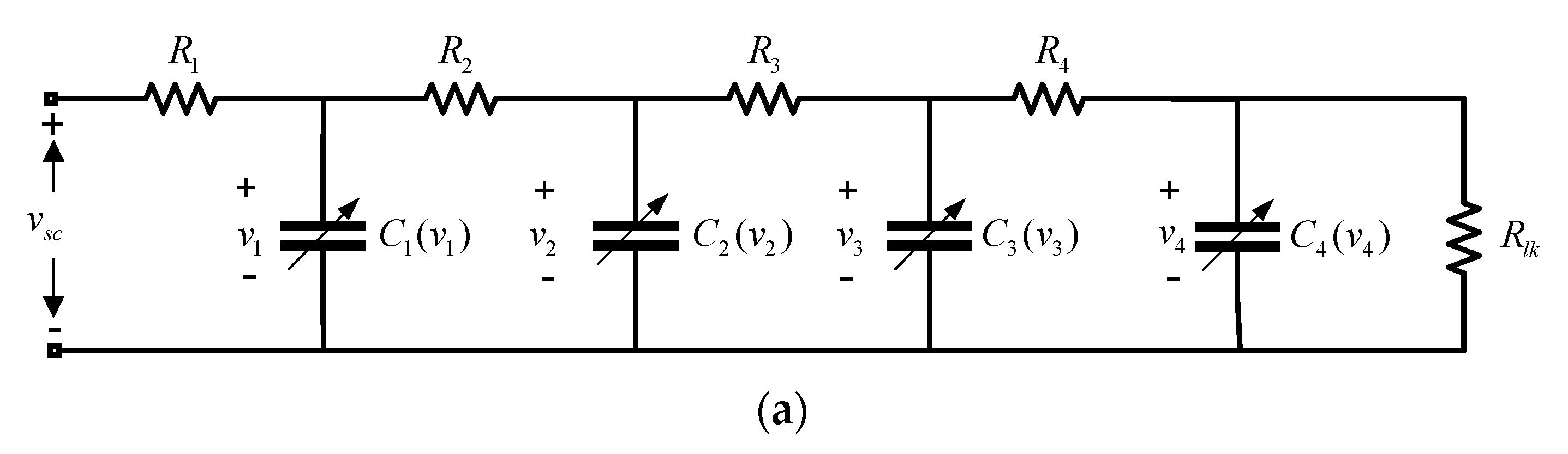
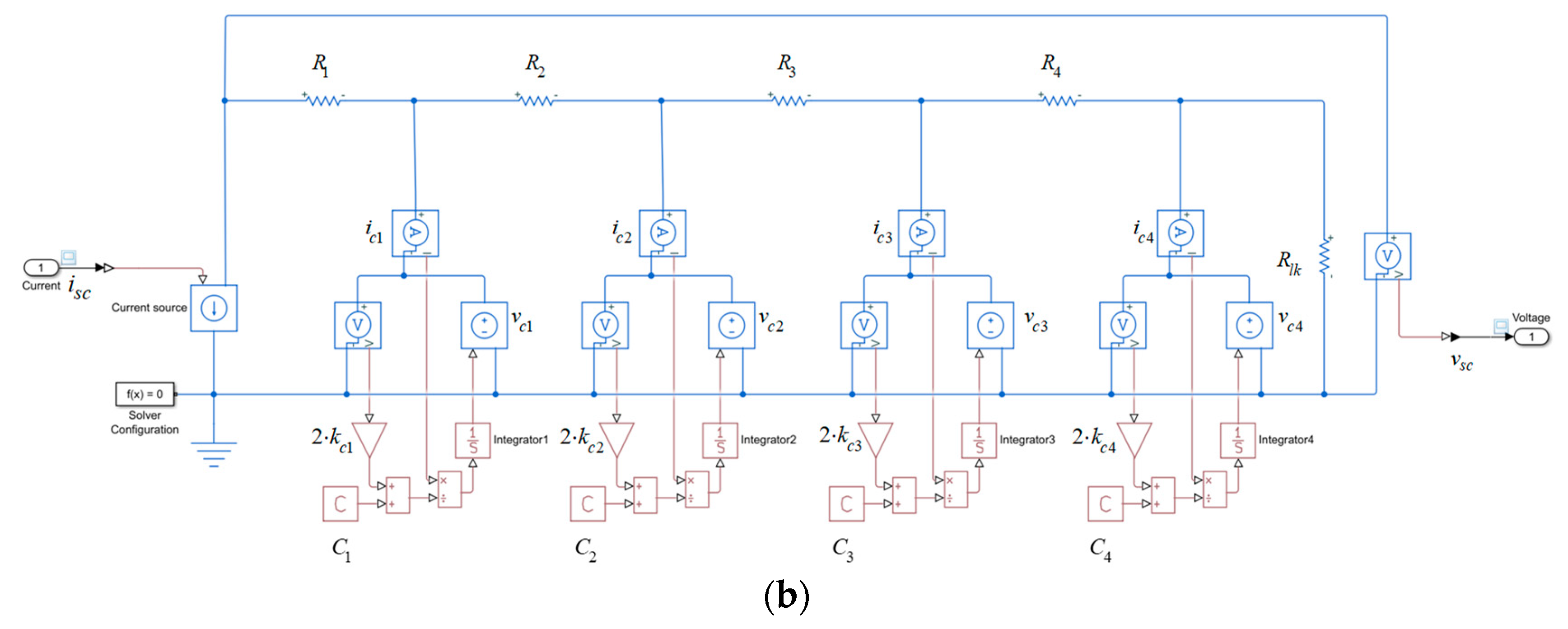
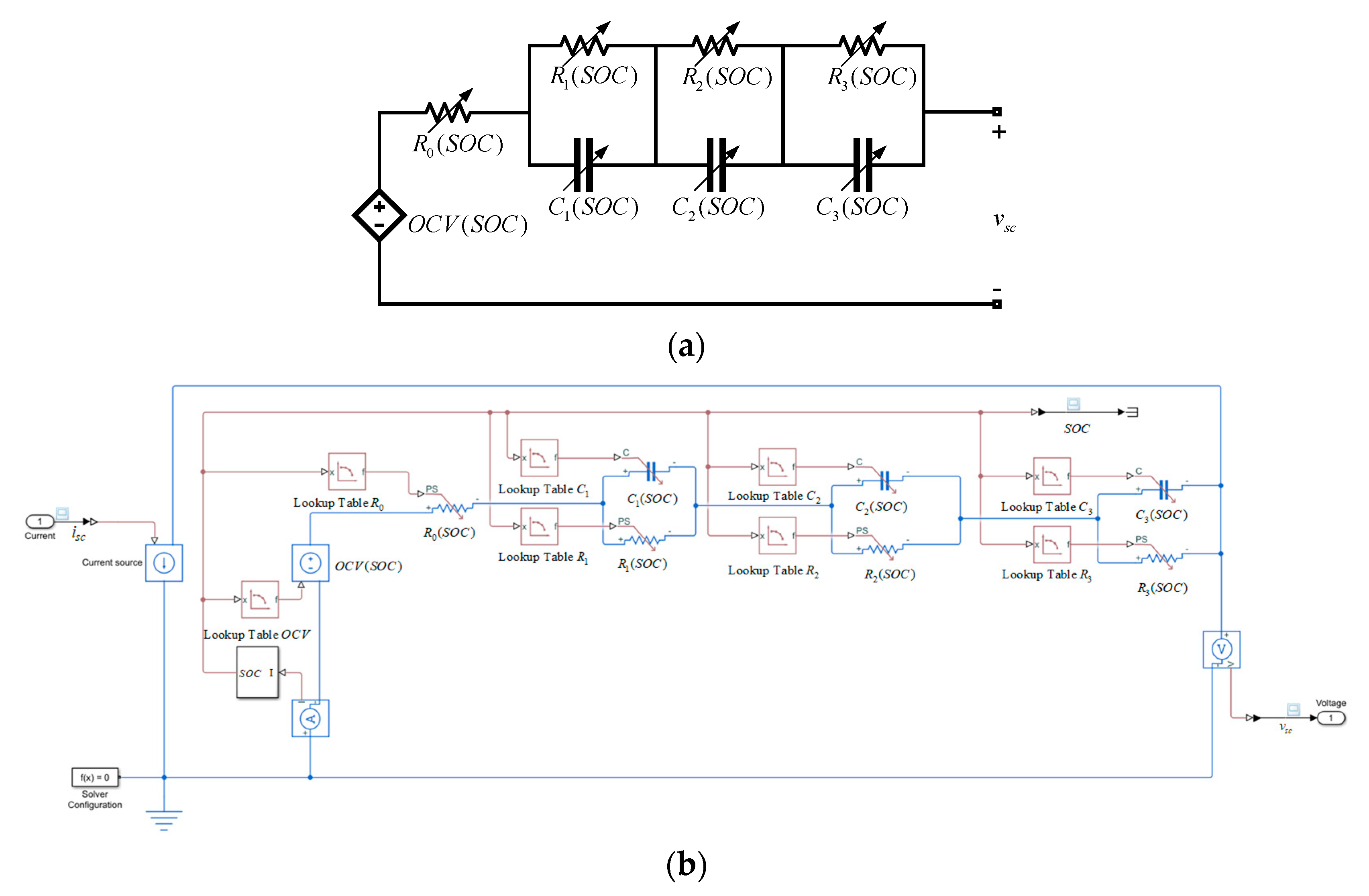
Section 2 shows the six supercapacitor models selected to make the comparative study, as well as their circuits implemented in Simulink or Simscape. Section 3 describes the parameters estimation procedure. 
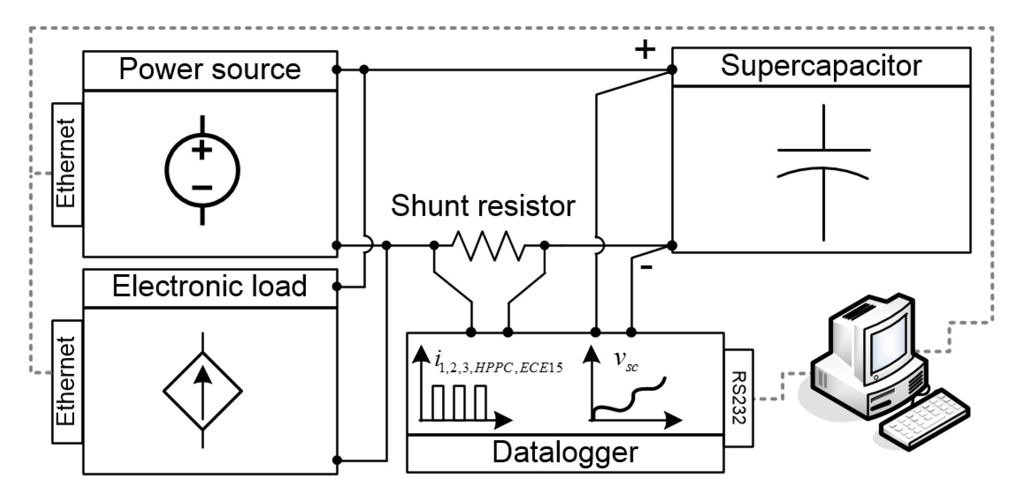
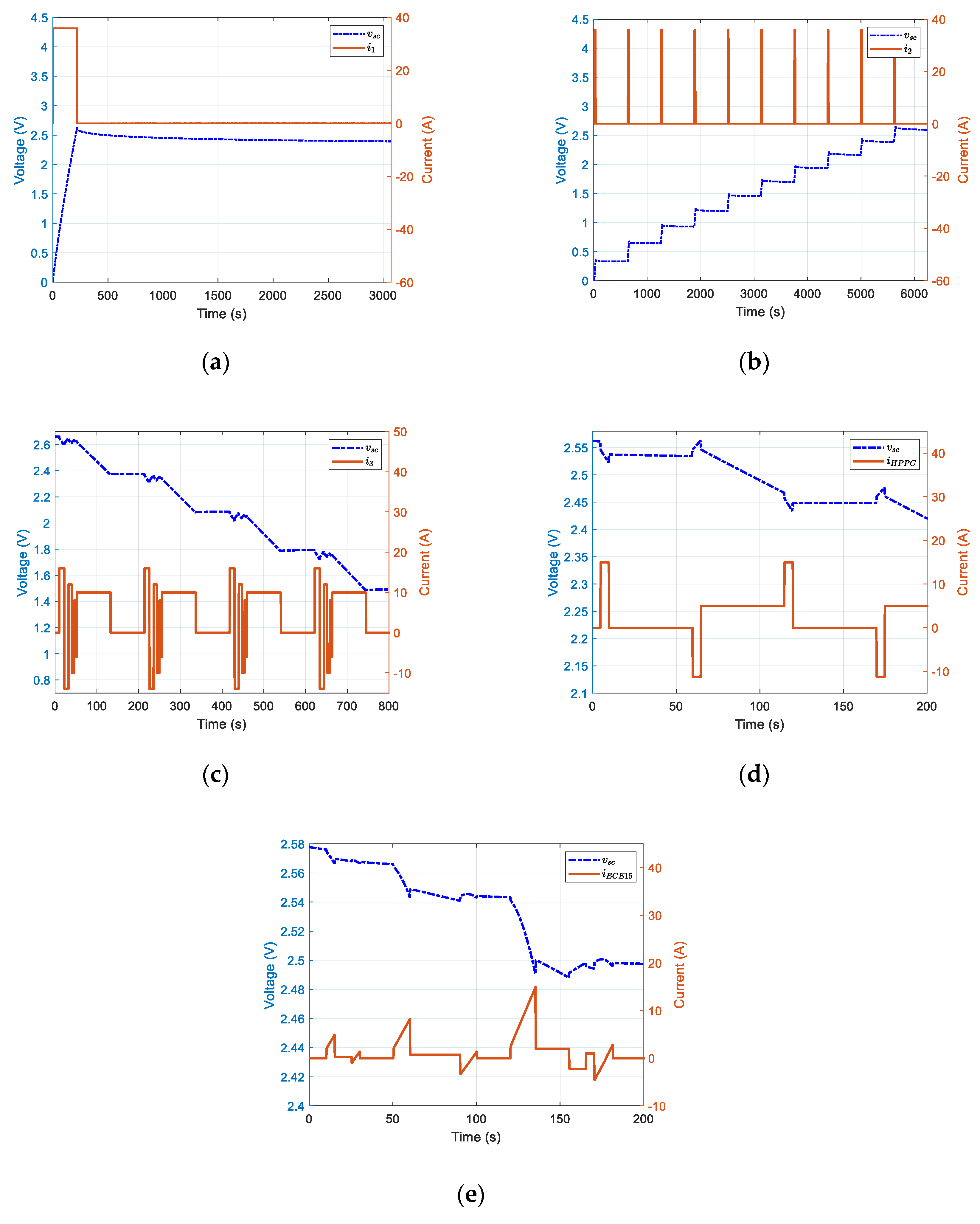
Section 4 depicted the different current profiles and the experimental setup to get the supercapacitor voltage and current responses. Section 5 shows the obtained statistical metrics using ECE15 and HPPC dynamic driving cycles, and the discussion about the experimental vs. simulation results. Finally, in Section 6, the main conclusions are presented.

2. Supercapacitors Models

In this section, six representative supercapacitor models are selected from the literature, which cover most of the typical applications. All of them are nonlinear models since this kind of models obtains better accuracy. The selected models are the Stern-Tafel Model [18], Zubieta Model [19], Series Model [20], Parallel Model [21], Transmission Line Model [22] and Thevenin Model [23]. In this section, the electrical equivalent circuit and the parameters of each model are reviewed.

2.1. Stern-Tafel Model

The supercapacitor proposed in reference [24] and reference [25] uses the Stern-Tafel model to describe the nonlinear capacitance. This electrochemical model reproduces the double layer capacitance (CT) related to the nonlinear diffusion dynamics. To do this, the supercapacitor model combines both the Helmholtz’s capacitance (CH) and Gouy-Chapman’s capacitance (CGC) [26],
C T = N p N s · ( 1 C H + 1 C G C ) 1
Being
C H = N e · ε · ε 0 · A i d
C G C = F · Q T 2 · N e · R · T s i n h ( Q T N e 2 · A i 8 · R · T · ε · ε 0 · c )
where Np is the number of parallel supercapacitor cells, Ns is the number of series of supercapacitor cells, Ne is the number of layers of electrodes, d the molecular radius (m), c the molar concentration (mol.m−3), Ai is the interfacial area between electrode and electrolyte (m2), T is the operating temperature (K), Fc is the Faraday constant (C/mol), R is the ideal gas constant (J/(K·mol)), ε is the relative permittivity of the electrolyte material (F/m), and ε0 is the free space permittivity (F/m) [18].
The model equivalent circuit has a controlled voltage source and an internal resistance, as shown in Figure 1a. This model depends on several parameters where Cn is the nominal capacitance (F), Vmax is the maximum supercapacitor voltage (V), Rdc is the internal resistance (Ω), VT is the total voltage (V), and isd is the self-discharge current (A) which is determined by the Tafel Equation (4) described in reference [27] as:
i s d ( t ) = N e · I f · e ( α · F c · ( V i n i t N s V m a x N s Δ V ) R · T )
where If is the leakage current (A), Vinit is the initial voltage (V), α is the charge transfer coefficient and ∆V is the over-potential (V). The capacitance of the electrochemical model requires only a few data from manufacturer datasheet and universal constant as described in reference [28]. The Simulink implementation is shown in Figure 1b.

2.2. Zubieta Model

The proposed model in reference [19] includes a circuit with three parallel RC time constant, Figure 2a. The first branch, with the elements R0C0, and the voltage-dependent kc·vc defines the response in seconds. The second branch R1C1 provides the response in the range of minutes. The branch R2C2 represents the response for a time longer than minutes. Finally, a resistor Rlk reproduces the leakage resistance.
A simplified equivalent circuit with two branches is shown in reference [29], with a simplified parameter identification procedure through the differential equation of the circuit. Similar studies are proposed in reference [30] in which the model parameters are easily obtained when the supercapacitor is discharged with constant power. In addition, reference [31] proposes a multivariable minimization function to find the parameters, they are validated with a current profile of a hybrid electric vehicle.
The total capacitance and current of the voltage-controlled capacitance implemented in Simscape are shown in Figure 2b, which are defined by (5) and (6):
C ( v c ) = C 0 + k c · v c
i c = d Q d t = d ( C ( v c ) · v c ) d t = ( C 0 + 2 k c · v c ) d v c d t
where C0 is the initial linear capacitance which represents the electrostatic capacitance of the capacitor, and kc a positive coefficient which represents the effects of the diffused layer of the supercapacitor.

2.3. Series Model

The series model is an equivalent circuit obtained through the AC impedance approach, which consists of two parallel RC circuit compound by R1(vsc), C1(vsc), R2(vsc), C2(vsc), connected in series with another RC circuit compound by Rs and Cs(vs), as described in references [20,32,33]. This equivalent circuit shows in the first branch of Figure 3a. In reference [34] a modified version of this circuit was presented, which includes the model proposed by Buller and Zubieta, in order to represent a complete model for a full frequency range. This complete model includes three branches in a parallel compound by R3 and C3, R4 and C4, and the leakage resistance Rlk, as shown in Figure 3a. Figure 3b shows the Simscape implementation of the modified series model.

2.4. Parallel Model

The basic parallel model with constant values is described in reference [35] and reference [36]. Reference [37] describes an approximation to calculate the parameters without data acquisition, only using the information provided by a supercapacitor datasheet, as well as the main basic equations to obtain the constant parameters using this information. A modified four parallel RC networks with voltage-dependent parameters are presented in reference [21], and it is shown in Figure 4a. This model is more complex, but it achieves better accuracy. Figure 4b shows the implementations of the modified parallel model in Simscape.

2.5. Transmission Line Model

Transmission line model is composed of nRC branches in order to reproduce the supercapacitor frequency response from 10 mHz to 1 kHz. This model was proposed for hybrid and electric vehicles, and it was described in reference [38] and reference [39]. This model consists of four parallel networks based on R1, C1(v1), R2, C2(v2), R3, C3(v3) and R4, C4(v4), and a parallel leakage resistance Rlk, as shown in Figure 5a. Reference [22] describes a procedure to estimate the parameters through time response and the equations of the circuit. Also, this model is used to evaluate the supercapacitor physical aging process [40], by estimating the uncertainties of the parameters. Reference [41] uses a different number of networks according to the simulation time step.
Figure 5b shows the model implemented in Simscape with the described Equations (5) and (6).

2.6. Thevenin Model

The equivalent electric circuit of the Thevenin model, which includes several parallel RC and a nonlinear state-of-charge (SOC) voltage-dependent source is described in reference [42]. The SOC is calculated by coulomb counting using (7):
S O C = Q i n i t 0 t i ( τ ) d τ Q T
with Qinit being the initial supercapacitor charge, QT being the total supercapacitor charge and i(τ) as the supercapacitor current.
In this paper, three RC branches are used to get a better accuracy, where OCV represents the open circuit voltage, R0 represents the internal resistance, and three parallel networks based on R1, C1, R2, C2, R3, and C3 reproduce the supercapacitor dynamic, as shown in Figure 6a. All parameters are state-of-charge dependent. The proposed model applied to a hybrid storage system for an electric vehicle gives a better agreement for a simulated vs. experimental response when 3-branches are used in the model [23]. Figure 6b shows the Simscape implementation.

3. Parameters Estimation Procedure

Parametric models explicitly contain differential equations, transfer function or block diagrams. The parameters update could be offline or online. For obtaining the parameters, in the offline mode, the data are stored to later process, on the other hand, in the online mode, the procedure is executed in parallel to the experiment [43]. In the literature, there are many proposed procedures to obtain the model parameters such as e.g., the unscented Kalman filter [44] or the Luenberger-style technique [17].
Taking into account the literature, this paper focuses on the proposal of a practical, interactive, simple and enough general offline procedures for estimating the model parameters.
Figure 7a shows the proposed identification procedure block diagram. This procedure can be divided into several steps, shown and described in Table 1.
In step 5, the optimization method has to be selected. This paper uses an offline parameters estimation based on the error minimization between the measured and simulated supercapacitor voltage. The iterative procedure tunes the supercapacitors model parameters (p) to get a simulated response (Vs) that tracks the measured response (Vm), with a finite number of samples (n). To do that, the solver minimizes the next cost function for each current profile:
F ( p ) = min p i = 0 n [ V m i V s i ( p ) ] 2
where p varies between zero and infinity (e.g., 0 to 1010).
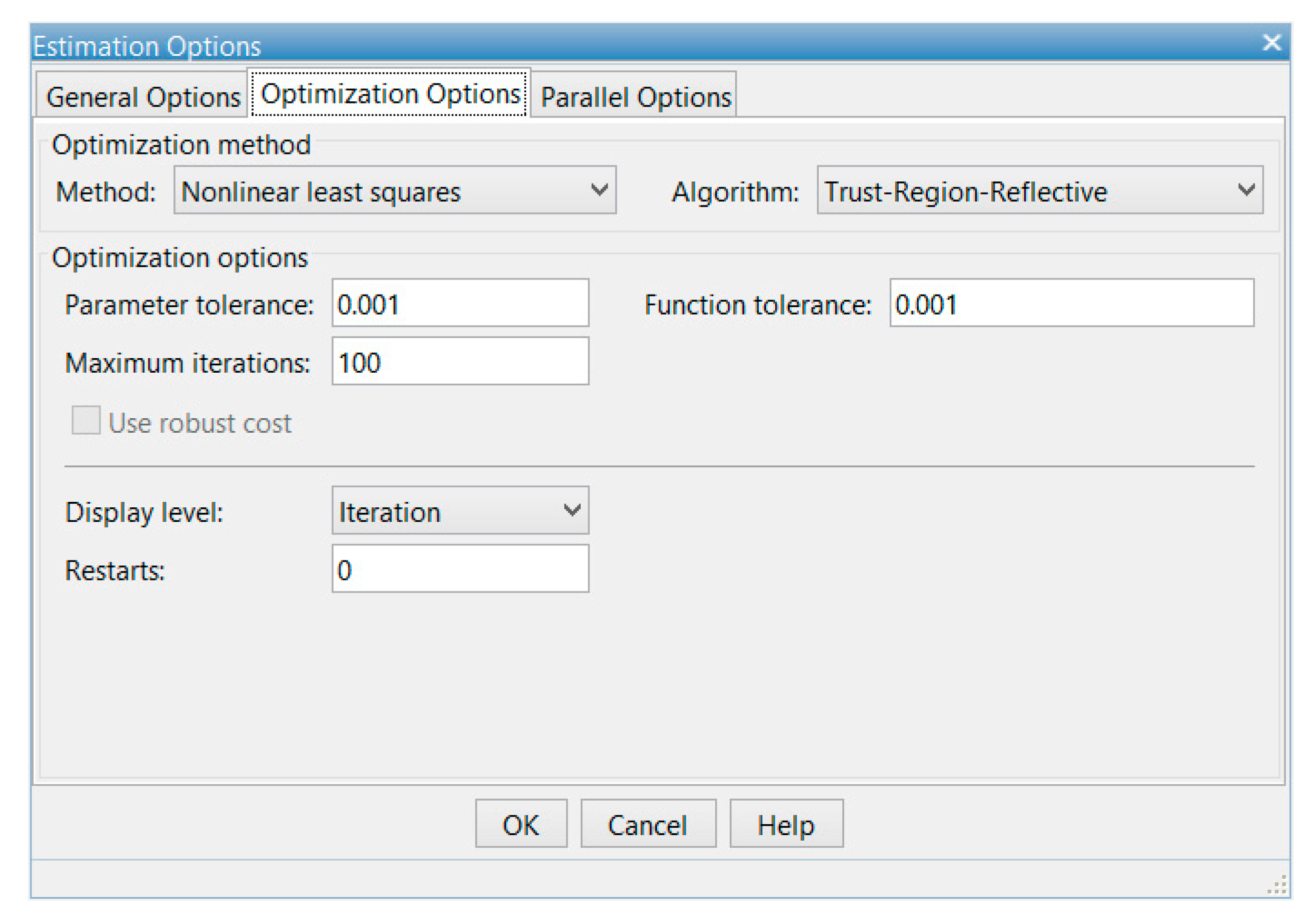
The minimization problem is carried out with Simulink® Design Optimization™ of Matlab (Version R2018b, MathWorks, Natick, MA, USA). This toolbox provides an interactive interface that helps to minimize the square of the error between the measured and simulated supercapacitor voltage, using the nonlinear least squares method for parameters estimation. This method is selected in the user interface as shown in Figure 8.
This method uses the Simulink function named as lsqnonlin, that requires at least (2k + 1) simulations per iteration, where k is the number of parameters to be estimated [46]. The required CPU time and memory increase as a function of the numbers of parameters and their initial values. The offline runtime estimation is in the order of minutes.
If runtime estimation has to be reduced, other techniques based on the layered technique to break the global optimization into a smaller task [47], or based on differential mutation strategy [48], or based on genetic programming [49], among others, could be used, although the flexibility and simplicity provided by the Simulink user interface could be affected.
On the other hand, the algorithm selected is the Trust-Region-Reflective, which is based on a gradient process with a trial step by solving a trust region. Specific details of the algorithm can be found in reference [45]. Additional information is detailed in reference [50], in which the process of how to import, analyze, prepare and estimate model parameters in Simulink is described.
Using the proposed procedure, based on Simulink® Design Optimization™ of Matlab, the most model can be built, from a practical point of view. Nevertheless, this procedure is limited by the optimization methods and algorithms included in Simulink.

4. Experimental Setup

4.1. Supercapacitor Testing System

The experimental setup includes a supercapacitor, a data acquisition system, a power source, and an electronic load, as shown in Figure 9. The supercapacitor used to develop the test has been the Maxwell BCAP3000. An equivalent bidirectional current source compound of the electronic load and the power source, connected in parallel, emulates the current profile. This equivalent current source includes the typical regenerative breaking present in automotive applications. The experimental current profile and the data acquisition system are conducted using the following set of equipment listed in Table 2:
All these elements have been synchronized with a computer running to manage the data logging and supervisory control using LabVIEW® software.

4.2. Supercapacitor Test Schedule

The parameter identification procedure uses three different current profiles. The current profile i1 is a current step, Figure 10a; the current profile i2 are repetitive charging current steps applied until to reach the maximum supercapacitor voltage, Figure 10b; and the current profile i3 is a dynamic charge-discharge current step modulated in amplitude and time applied until the middle value of the supercapacitor voltage range, [51], Figure 10c. From the modeling perspective, the validation current profile must be more dynamic in amplitude and frequency than the identification current profile, as shown in Figure 10d,e.
These identification current profiles apply to those models aforementioned in Section 2 to obtain their parameters. The current profile applied in every model is shown in Table 3.
The robustness and accuracy of the supercapacitor models are evaluated by means of different standardized test profiles, which include the Hybrid Pulse Power Characterization (HPPC) test and European Urban Driving Cycle (ECE15) for long-time responses. Figure 9d shows the HPPC test that is described in the Freedom Car Battery Manual [52]. The ECE15 test, described in reference [53], is a more dynamic current profile, as shown in Figure 10e.

5. Experimental Results, Comparison, and Discussion

After obtaining the parameters for each model, detailed in Appendix A in Table A1, Table A2, Table A3, Table A4, Table A5, Table A6, Table A7, Table A8 and Table A9, using the procedure described in Section 3 and identification current profiles described in Section 4, the output voltage accuracy and robustness analysis for the six supercapacitor models described in Section 2 is performed based on statistical metrics, such as relative error and root-mean-square (RMS) error.
Comparative results with identification current profile i1 are illustrated in Figure 11a–d for the HPPC test and Figure 11e–h for the ECE15 test. Figure 11a,e show the experimental supercapacitor voltage and the voltages provided by the Stern-Tafel and Zubieta models. Figure 11b,f show the relative error between these models and the experimental data.
Figure 11c,g represent the relative error in percentage. Figure 11d,h show the RMS error in mV. It shows that the Stern-Tafel model has lower error values in comparison with the Zubieta model. In any case, the relative error tendency with the time increase in both models, therefore the accuracy of both models identified with the i1 current profile is not proper.
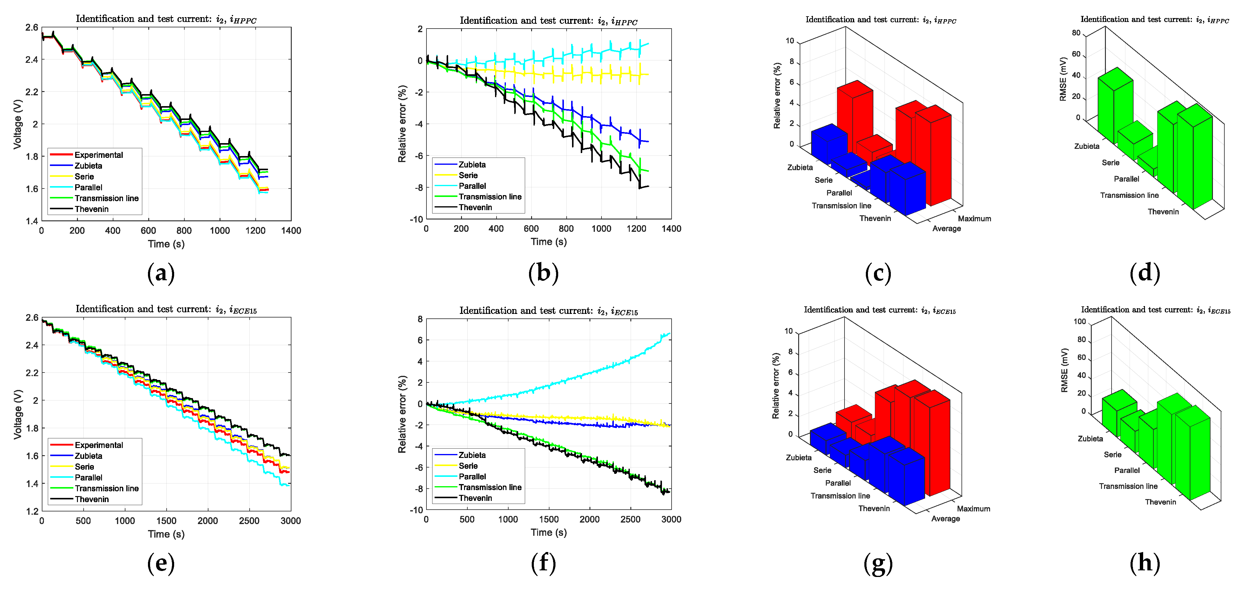
Similar information is shown when current profile i2 is used to obtain the model parameters. Figure 12a–d depicted the obtained result for the HPPC test and Figure 12e–h for the ECE15 test. This current profile is applied to five out of the six models, with the exception of the Stern-Tafel model. In this case, the Series model is the best one, since it presents a reduced relative error that maintained with the time.
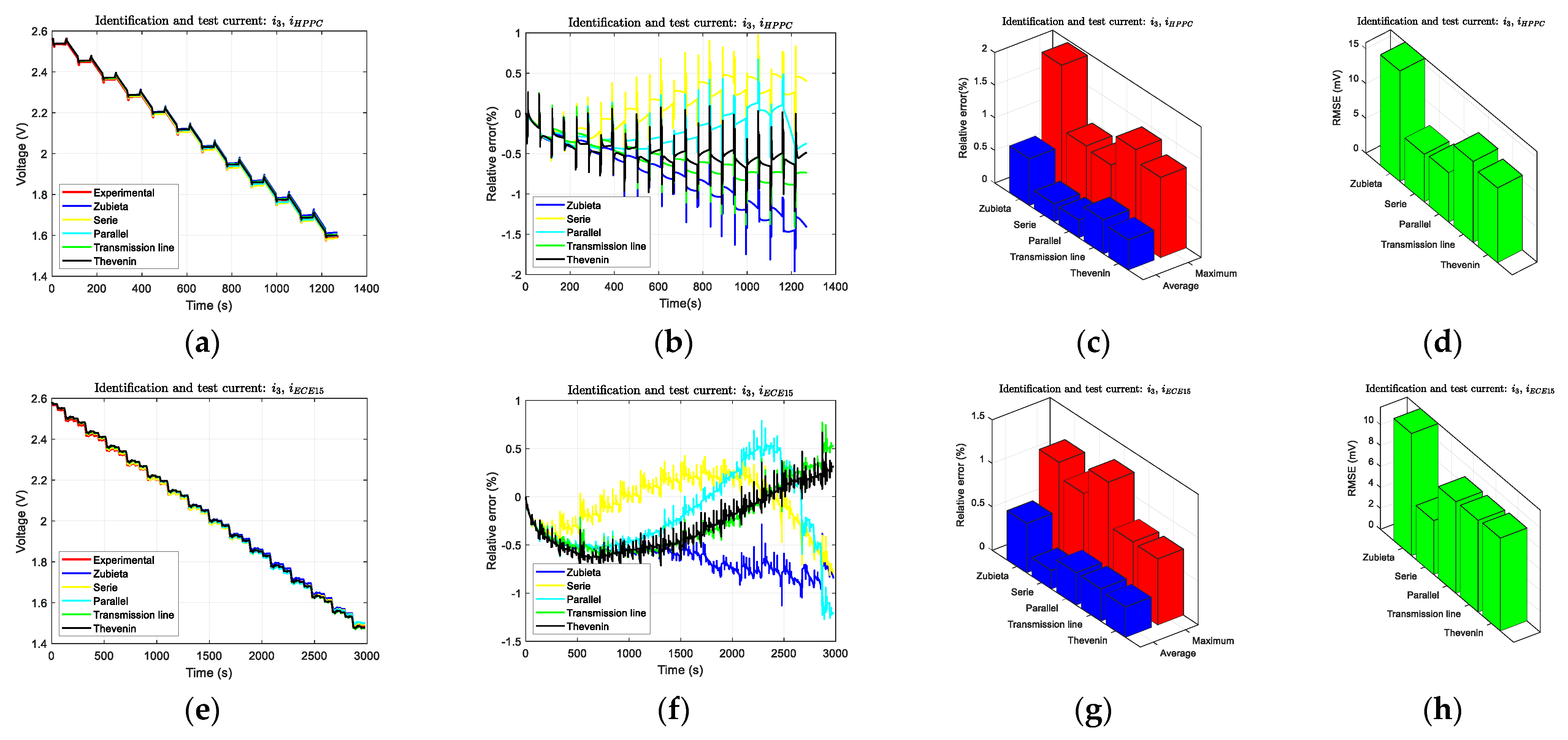
Finally, the result obtained with the current profile i3, which is the most dynamic current profile, is depicted in Figure 13a–d for the HPPC test and Figure 13e–h for the ECE15 test. This current profile has been applied to the same models as current profile i2. Again, the Serie Model has the best performance, and even the obtained relative error is lower than using the previous current profiles. Nevertheless, the Parallel model, Transmission Line model and Thevenin model get good behaviors.
The main conclusions obtained from these results are the following:
  • The greater complex identification current profile i3 gets greater accuracy for every model in which it can be applied.
  • In most cases, the Series model provides the minimum relative error.
  • If a simple and basic supercapacitor model has to be used, the best option is to use Zubieta model identified with the current profile i3.
Table 4, Table 5 and Table 6 include the numeric values for different current profiles identification and the response of each model for HPPC and ECE15 test. These values are those shown in Figure 10, Figure 11 and Figure 12.

6. Conclusions

This paper describes a parameter identification general procedure with a flexible and interactive interface used to build supercapacitor models in Simulink or Simscape. This procedure enables estimating the different models parameters based on the use of the Optimization Toolbox of Matlab®. Once, the procedure steps are explained, the procedure is used to develop a comparative study of six commonly used supercapacitor models. In addition, the procedure enables using different identification current profiles, providing the possibility of analyzing the influence of three different identification current profiles in the accuracy and robustness of every model.
The experimental results obtained from the six models and three different identification current profiles, used to develop the study, show that both the model and the identification current profile are critical to obtaining good accuracy and robustness, which must be maintained over time.
From the comparison between the experimental results and the simulation results obtained using the model, it can be concluded that the greater complexity of the current identification profile, the greater accuracy and robustness of the model. In this case, the most complex identification current profile i3 gets the best accuracy for every model in which it can be applied.
In a short simulation period, most models provide enough accuracy results. However, in a long simulation period the differences among models as well as among the current identification profiles increase, and models responses cumulate voltage errors and, in some cases, they cannot correctly represent the voltage of the supercapacitor. The Stern-Tafel model is proper for a short simulation and as a first approximation. However, in a long-time simulation, the Series Model represents a good performance, followed by the Parallel Model. In most cases, the Series model provides the minimum relative error. However, the Zubieta model provides a good compromise between complexity and accuracy. Then, if a simple and basic supercapacitor model has to be used, the best option is to use a Zubieta model identified by means of the current profile i3.

Author Contributions

Conceptualization, H.M. and A.B.; methodology, A.B.; software, H.M.; validation, A.B., P.Z. and A.L.; formal analysis, C.F.; resources, A.B.; writing—original draft preparation, H.M.; writing—review and editing, P.Z. and A.L.; supervision, C.F.; funding acquisition, A.B.

Funding

This research was funded by the Spanish Ministry of Economy and Competitiveness and ERDF, grant number DPI2014-53685-C2-1-R.

Acknowledgments

This work has been supported by the Ministry of Economy and Competitiveness and FEDER funds through the research project “Storage and Energy Management for Hybrid Electric Vehicles based on Fuel Cell, Battery and Supercapacitors”—ELECTRICAR-AG-(DPI2014-53685-C2-1-R).

Conflicts of Interest

The authors declare no conflicts of interest.

Appendix A. Tables of Supercapacitors Parameter

Table A1. Stern-Tafel Model Parameters with current profile i1.
ParameterValue
C (F)3000
Rdc (mΩ)2.1000
If (mA)5.2000
Vn (V)2.7000
Ns1
Np1
Ne *2
d (nm) *1.0115
α *0.3200 (0 < α < 1)
V *0.4100
* = Estimated parameters.
Table A2. Zubieta Model Parameters.
ParameterCurrent Profile
i1i2i3
R0 (mΩ) *1.10800.86530.6504
C0 (F) *2290.30002172.60002081.7000
kc (F/V) *244.4400240.5600220.1800
R1 (Ω) *16.913019.928010.5170
C1 (F) *471.1500368.1700111.1500
R2 (Ω) *0.67290.37733.5770
C2 (F) *292.0100176.3200382.0700
Rlk (kΩ) *1712101102351.4030
* = Estimated parameters.
Table A3. Series Model Parameters with current profile i2.
ParameterVoltage (V)
00.3300.64170.92951.19771.45221.69731.9342.16222.38302.5948
Cs (kΩ) *2.46552.36292.54192.66992.82602.89412.94502.9623.06663.15183.5999
R1 (µΩ) *581.02470.26563.94546.61540.87507.120544.94238.40.00801.37311.6410
C1 (kF) *1.15951.70941.02851.57021.56952.15291.44290.277265.98065.88487.292
R2 (µΩ) *0.12058.12614.81025.84243.970108.8700.01646.128707.200692.73501.860
C2 (F) *14.39313241891.110714570.4234.540058.91913.5143.7690161.8454.3090
R3 (Ω) *10.6610
C3 (kF) *1.0877
R4 (Ω) *14.4660
C4 (F) *32.5750
Rlk (kΩ) *5.5436
* = Estimated parameters.
Table A4. Series Model Parameters with current profile i3.
ParameterVoltage (V)
1.49321.79312.08742.37612.6618
Cs (kΩ) *2.88902.96263.04893.17453.1935
R1 (µΩ) *192.3800460.1300428.0600182.1800437.5600
C1 (F) *15.3320923.850030.60209.3121229.6200
R2 (µΩ) *166.37001.411432.8880303.260099.7610
C2 (kF) *0.03090.21201.93801.99370.1050
R3 (Ω) *7.6440
C3 (kF) *1.2486
R4 (Ω) *14.0350
C4 (F) *110.7000
Rlk (kΩ) *1584.4000
* = Estimated parameters.
Table A5. Parallel Model Parameters with current profile i2.
ParameterVoltage (V)
0.00020.33010.64170.92951.19771.45221.69731.93372.16222.38302.5948
C1 (kF) *11.49456.4786.8260.225482.2030.00353100.120219.83125.880182.96170
R1 (Ω) *1850291.5431980.415.8680421.902545.451657857.68398.850254.02279.950
C2 (F) *561.28258.20362.59239.44057.131065.96956.8820112.78134.45046.67650.050
R2 (mΩ) *0.0035811.9370.37571.9524155.180137.89117.09014.30813.7464622.1500.020
C3 (F) *1068.91780.70.345843.196047.33200.1059665.2608.36712.69130.79825.003
R3 (mΩ) *2.93115.58320.000140.622316.9463.01615.61901.25790.01369369.01100
C4 (kF) *1.80160.04522.43502.43552.79392.76222.45723.0133.06413.30263.119
R4 (mΩ) *6.47378.40520.14411.04500.58370.63550.64290.40830.30570.57580.199
Rlk (Ω) *1.678615.39713.82925.629011.71413.70117.80117.82116.06516.64918.947
* = Estimated parameters.
Table A6. Parallel Model Parameters with current profile i3.
ParameterVoltage (V)
1.49321.79312.08742.37612.6618
C1 (kF) *21.1090652.920119.440503.49028.4650
R1 (Ω) *0.3961765.50364.790112.37014.1460
C2 (F) *59.1990123.90110.42126.43026.3940
R2 (Ω) *9.17860.126050.119930.092050.01963
C3 (F) *657.71015.92021.984017.628015.6860
R3 (mΩ) *16.00704.710511.43400.061512.3470
C4 (kF) *3.07462.8672.93473.03513.1868
R4 (uΩ) *507.890657.90689.490470.030850.340
Rlk (Ω) *120.930768.8106150.30585.340303.670
* = Estimated parameters.
Table A7. Transmission Line Model Parameters.
ParameterCurrent Profile
i2i3
R1 (µΩ) *826.72575.75
R2 (mΩ) *115.672.7568
R3 (Ω) *1.35580.0116
R4 (Ω) *3.96211.5723
kc1 (F/V) *209.2085.715
kc2 (F/V) *26.608021.482
kc3 (F/V) *47.151013.4470
kc4 (F/V) *11.854015.2340
C1 (F) *2303.302408.90
C2 (F) *0.10005.2926
C3 (F) *21.2820120.67
C4 (F) *37.901055.4780
Rlk (kΩ) *111.0113.8080
* = Estimated parameters.
Table A8. Thevenin Model Parameters with i2 Current Profile.
ParameterSOC (%)
0.011020.0429.9639.9549.8659.8969.7770.7789.6799.64
OCV (V)0.00020.3300.64170.92951.19771.45221.69731.93372.1622.38302.5953
C1 (F) *17046551.64236.58303.76363.06509.86434.30401.51227.47411.24147.11
C2 (kF) *119.2829.5835.42730.32339.52722.57920.577771.5711.61494.52219.695
C3 (kF) *2943.8498.12248.36205.07541.22449.09844.1697.2522507.5703.253.772
R0 (µΩ) *723.2431.020.247613.381104.4117.203.7923213.26115.9623.528372.15
R1 (mΩ) *1.24360.94161.25041.16901.19981.36761.34951.23951.08541.10861.2487
R2 (mΩ) *68.62210.2611.181935.6483.34910.324050.45297.775414.92501.6529186.44
R3 (Ω) *33.59222.7650.90592.1432.68651.9369432.48054814029422558.260555
* = Estimated parameters.
Table A9. Thevenin Model Parameters with i3 Current Profile.
ParameterSOC (%)
53.3764.6875.9787.2598.59
OCV (V)1.47861.77942.07422.3652.6499
C1 (F) *0.07073111.161011.161012.30123.90
C2 (kF) *7.27091.33620.790716.10728.906
C3 (MF) *1929.300.007690.0063876.58009.8952
R0 (µΩ) *6.516713.910039.474075.854053.527
R1 (µΩ) *204.02168.9735.226339.940565.850
R2 (µΩ) *684.340486.780512.330352.520284.940
R3 (µΩ) *24.67104.84917.873074.05600.25154
* = Estimated parameters.

References

  1. Zhang, L.; Hu, X.; Wang, Z.; Sun, F.; Dorrell, D.G. A review of supercapacitor modeling, estimation, and applications: A control/management perspective. Renew. Sustain. Energy Rev. 2018, 81, 1868–1878. [Google Scholar] [CrossRef]
  2. Ristic, M.; Gryska, Y.; McGinley, J.V.; Yufit, V. Supercapacitor energy storage for magnetic resonance imaging systems. IEEE Trans. Ind. Electron. 2014, 61, 4255–4264. [Google Scholar] [CrossRef]
  3. Wu, W.; Partridge, J.; Bucknall, R. Development and Evaluation of a Degree of Hybridisation Identification Strategy for a Fuel Cell Supercapacitor Hybrid Bus. Energies 2019, 12, 142. [Google Scholar] [CrossRef]
  4. Ciccarelli, F.; Di Noia, L.; Rizzo, R. Integration of Photovoltaic Plants and Supercapacitors in Tramway Power Systems. Energies 2018, 11, 410. [Google Scholar] [CrossRef]
  5. Vazquez, S.; Lukic, S.M.; Galvan, E.; Franquelo, L.G.; Carrasco, J.M. Energy storage systems for transport and grid applications. IEEE Trans. Ind. Electron. 2010, 57, 3881–3895. [Google Scholar] [CrossRef]
  6. Yang, X.; Wen, P.; Xue, Y.; Zheng, T.; Wang, Y. Supercapacitor energy storage based MMC for energy harvesting in mine hoist application. Energies 2017, 10, 1428. [Google Scholar] [CrossRef]
  7. Yang, H.; Zhang, Y. A study of supercapacitor charge redistribution for applications in environmentally powered wireless sensor nodes. J. Power Sources 2015, 273, 223–236. [Google Scholar] [CrossRef]
  8. Wang, H.; Zhou, Q.; Yao, B.; Ma, H.; Zhang, M.; Li, C.; Shi, G. Suppressing the Self-Discharge of Supercapacitors by Modifying Separators with an Ionic Polyelectrolyte. Adv. Mater. Interfaces 2018, 5, 1701547. [Google Scholar] [CrossRef]
  9. Xia, M.; Nie, J.; Zhang, Z.; Lu, X.; Wang, Z.L. Suppressing self-discharge of supercapacitors via electrorheological effect of liquid crystals. Nano Energy 2018, 47, 43–50. [Google Scholar] [CrossRef]
  10. Sarwar, W.; Marinescu, M.; Green, N.; Taylor, N.; Offer, G. Electrochemical double layer capacitor electro-thermal modelling. J. Energy Storage 2016, 5, 10–24. [Google Scholar] [CrossRef] [Green Version]
  11. Wang, H.; Pilon, L. Mesoscale modeling of electric double layer capacitors with three-dimensional ordered structures. J. Power Sources 2013, 221, 252–260. [Google Scholar] [CrossRef]
  12. Lee, J.; Yi, J.; Kim, D.; Shin, C.; Min, K.S.; Choi, J.; Lee, H.Y. Modeling of the Electrical and Thermal Behaviors of an Ultracapacitor. Energies 2014, 7, 8264–8278. [Google Scholar] [CrossRef] [Green Version]
  13. Zhang, L.; Wang, Z.; Hu, X.; Sun, F.; Dorrell, D.G. A comparative study of equivalent circuit models of ultracapacitors for electric vehicles. J. Power Sources 2015, 274, 899–906. [Google Scholar] [CrossRef]
  14. Shi, L.; Crow, M. Comparison of ultracapacitor electric circuit models. In Proceedings of the IEEE Power and Energy Society General Meeting—Conversion and Delivery of Electrical Energy in the 21st Century, Pittsburgh, PA, USA, 20–24 July 2008; pp. 1–6. [Google Scholar]
  15. Xie, C.; Liu, X.; Huang, L.; Fang, W. Modeling of supercapacitor modules in the hybrid powertrain with a nonlinear 3-branch equivalent circuit. Int. J. Energy Res. 2018, 42, 3524–3534. [Google Scholar] [CrossRef]
  16. Miniguano, H.; Raga, C.; Barrado, A.; Lázaro, A.; Zumel, P.; Olías, E. A comparative study and parameterization of electrical battery models applied to hybrid electric vehicles. In Proceedings of the International Conference on Electrical Systems for Aircraft, Railway, Ship Propulsion and Road Vehicles & International Transportation Electrification Conference (ESARS-ITEC), Toulouse, France, 2–4 November 2016; pp. 1–6. [Google Scholar]
  17. Ceraolo, M.; Lutzemberger, G.; Poli, D. State-Of-Charge Evaluation Of Supercapacitors. J. Energy Storage 2017, 11, 211–218. [Google Scholar] [CrossRef]
  18. Motapon, S.N.; Dessaint, L.A.; Al-Haddad, K. A comparative study of energy management schemes for a fuel-cell hybrid emergency power system of more-electric aircraft. IEEE Trans. Ind. Electron. 2014, 61, 1320–1334. [Google Scholar] [CrossRef]
  19. Zubieta, L.; Bonert, R. Characterization of double-layer capacitors for power electronics applications. IEEE Trans. Ind. Appl. 2000, 36, 199–205. [Google Scholar] [CrossRef] [Green Version]
  20. Wu, C.; Hung, Y.; Hong, C. On-line supercapacitor dynamic models for energy conversion and management. Energy Convers. Manag. 2012, 53, 337–345. [Google Scholar] [CrossRef]
  21. Quintáns, C.; Iglesias, R.; Lago, A.; Acevedo, J.M.; Martínez-Peñalver, C. Methodology to obtain the voltage-dependent parameters of a fourth-order supercapacitor model with the transient response to current pulses. IEEE Trans. Power Electron. 2017, 32, 3868–3878. [Google Scholar] [CrossRef]
  22. Noh, S.; Choi, J.; Kim, H.C.; Lee, E.K. PSIM Based electric modeling of supercapacitors for line voltage regulation of electric train system. In Proceedings of the EEE 2nd International Power and Energy Conference, Johor Bahru, Malaysia, 1–3 December 2008; pp. 855–859. [Google Scholar]
  23. Michalczuk, M.; Grzesiak, L.M.; Ufnalski, B. Experimental parameter identification of battery-ultracapacitor energy storage system. In Proceedings of the IEEE 24th International Symposium on Industrial Electronics (ISIE), Buzios, Brazil, 3–5 June 2015; pp. 1260–1265. [Google Scholar]
  24. Kang, J.; Wen, J.; Jayaram, S.H.; Yu, A.; Wang, X. Development of an equivalent circuit model for electrochemical double layer capacitors (EDLCs) with distinct electrolytes. Electrochim. Acta 2014, 115, 587–598. [Google Scholar] [CrossRef]
  25. Xu, N.; Riley, J. Nonlinear analysis of a classical system: The double-layer capacitor. Electrochem. Commun. 2011, 13, 1077–1081. [Google Scholar] [CrossRef]
  26. Oldham, K.B. A Gouy–Chapman–Stern model of the double layer at a (metal)/(ionic liquid) interface. J. Electroanal. Chem. 2008, 613, 131–138. [Google Scholar] [CrossRef]
  27. Conway, B.E.; Pell, W.; Liu, T. Diagnostic analyses for mechanisms of self-discharge of electrochemical capacitors and batteries. J. Power Sources 1997, 65, 53–59. [Google Scholar] [CrossRef]
  28. Ji, H.; Zhao, X.; Qiao, Z.; Jung, J.; Zhu, Y.; Lu, Y.; Zhang, L.L.; MacDonald, A.H.; Ruoff, R.S. Capacitance of carbon-based electrical double-layer capacitors. Nat. Commun. 2014, 5, 3317. [Google Scholar] [CrossRef] [Green Version]
  29. Faranda, R. A new parameters identification procedure for simplified double layer capacitor two-branch model. Electr. Power Syst. Res. 2010, 80, 363–371. [Google Scholar] [CrossRef]
  30. Yang, H.; Zhang, Y. Characterization of supercapacitor models for analyzing supercapacitors connected to constant power elements. J. Power Sources 2016, 312, 165–171. [Google Scholar] [CrossRef]
  31. Solano, J.; Hissel, D.; Pera, M.C. Modeling and parameter identification of ultracapacitors for hybrid electrical vehicles. In Proceedings of the IEEE Vehicle Power and Propulsion Conference (VPPC), Beijing, China, 15–18 October 2013; pp. 1–4. [Google Scholar]
  32. Kim, S.H.; Choi, W.; Lee, K.B.; Choi, S. Advanced dynamic simulation of supercapacitors considering parameter variation and self-discharge. IEEE Trans. Power Electron. 2011, 26, 3377–3385. [Google Scholar]
  33. Buller, S.; Karden, E.; Kok, D.; De Doncker, R. Modeling the dynamic behavior of supercapacitors using impedance spectroscopy. In Proceedings of the Conference Record of the 2001 IEEE Industry Applications Conference. 36th IAS Annual Meeting (Cat. No.01CH37248), Chicago, IL, USA, 30 September–4 October 2001; Volume 4, pp. 2500–2504. [Google Scholar]
  34. Musolino, V.; Piegari, L.; Tironi, E. New Full-Frequency-Range Supercapacitor Model With Easy Identification Procedure. IEEE Trans. Ind. Electron. 2013, 60, 112–120. [Google Scholar] [CrossRef]
  35. Signorelli, R.; Ku, D.C.; Kassakian, J.G.; Schindall, J.E. Electrochemical Double-Layer Capacitors Using Carbon Nanotube Electrode Structures. Proc. IEEE 2009, 97, 1837–1847. [Google Scholar] [CrossRef]
  36. Wei, T.; Qi, X.; Qi, Z. An improved ultracapacitor equivalent circuit model for the design of energy storage power systems. In Proceedings of the International Conference on Electrical Machines and Systems (ICEMS), Seoul, South Korea, 8–11 October 2007; pp. 69–73. [Google Scholar]
  37. Miller, J.M.; McCleer, P.J.; Cohen, M. Ultracapacitors as Energy Buffers in a Multiple Zone Electrical Distribution System; Maxwell Technologies: San Diego, CA, USA, 2004. [Google Scholar]
  38. Lajnef, W.; Vinassa, J.M.; Briat, O.; Azzopardi, S.; Woirgard, E. Characterization methods and modelling of ultracapacitors for use as peak power sources. J. Power Sources 2007, 168, 553–560. [Google Scholar] [CrossRef]
  39. Yang, H. Estimation of Supercapacitor Charge Capacity Bounds Considering Charge Redistribution. IEEE Trans. Power Electron. 2018, 33, 6980–6993. [Google Scholar] [CrossRef]
  40. Schaeffer, E.; Auger, F.; Shi, Z.; Guillemet, P.; Loron, L. Comparative analysis of some parametric model structures dedicated to EDLC diagnosis. IEEE Trans. Ind. Electron. 2016, 63, 387–396. [Google Scholar] [CrossRef]
  41. Dougal, R.; Gao, L.; Liu, S. Ultracapacitor model with automatic order selection and capacity scaling for dynamic system simulation. J. Power Sources 2004, 126, 250–257. [Google Scholar] [CrossRef]
  42. Parvini, Y.; Siegel, J.B.; Stefanopoulou, A.G.; Vahidi, A. Supercapacitor electrical and thermal modeling, identification, and validation for a wide range of temperature and power applications. IEEE Trans. Ind. Electron. 2016, 63, 1574–1585. [Google Scholar] [CrossRef]
  43. Isermann, R.; Münchhof, M. Identification of Dynamic Systems: An Introduction with Applications; Springer Science & Business Media: Berlin, Germany, 2010. [Google Scholar]
  44. Wang, Y.; Liu, C.; Pan, R.; Chen, Z. Modeling and state-of-charge prediction of lithium-ion battery and ultracapacitor hybrids with a co-estimator. Energy 2017, 121, 739–750. [Google Scholar] [CrossRef]
  45. MathWorks. Simulink® Design Optimization User ’s Guide; MathWorks: Natick, MA, USA, 2018. [Google Scholar]
  46. Jackey, R.A.; Plett, G.L.; Klein, M.J. Parameterization of a Battery Simulation Model Using Numerical Optimization Methods; Technical Report; SAE: Warrendale, PA, USA, 2009. [Google Scholar]
  47. Jackey, R.; Saginaw, M.; Sanghvi, P.; Gazzarri, J.; Huria, T.; Ceraolo, M. Battery Model Parameter Estimation Using a Layered Technique: An Example Using a Lithium Iron Phosphate Cell; Technical Report; SAE: Warrendale, PA, USA, 2013. [Google Scholar]
  48. Chakraborty, U.K.; Abbott, T.E.; Das, S.K. PEM fuel cell modeling using differential evolution. Energy 2012, 40, 387–399. [Google Scholar] [CrossRef]
  49. Chakraborty, U.K. Static and dynamic modeling of solid oxide fuel cell using genetic programming. Energy 2009, 34, 740–751. [Google Scholar] [CrossRef]
  50. MathWorks. Simulink® Design Optimization Getting Started Guide; MathWorks: Natick, MA, USA, 2019. [Google Scholar]
  51. Burke, A. Ultracapacitor technologies and application in hybrid and electric vehicles. Int. J. Energy Res. 2010, 34, 133–151. [Google Scholar] [CrossRef]
  52. He, H.; Xiong, R.; Zhang, X.; Sun, F.; Fan, J. State-of-charge estimation of the lithium-ion battery using an adaptive extended Kalman filter based on an improved Thevenin model. IEEE Trans. Veh. Technol. 2011, 60, 1461–1469. [Google Scholar]
  53. Raga, C.; Barrado, A.; Lázaro, A.; Quesada, I.; Sanz, M.; Zumel, P. Driving profile and fuel cell minimum power analysis impact over the size and cost of fuel cell based propulsion systems. In Proceedings of the 9th International Conference on Compatibility and Power Electronics (CPE), Costa da Caparica, Portugal, 24–26 June 2015; pp. 390–395. [Google Scholar]
Figure 1. Stern-Tafel model: (a) Electric circuit; (b) Simulink implementation.
Energies 12 01776 g001
Figure 2. Zubieta model: (a) Electric circuit; (b) Simscape implementation.
Energies 12 01776 g002
Figure 3. Series model: (a) Electric circuit; (b) Simscape implementation.
Energies 12 01776 g003
Figure 4. Series model: (a) Electric circuit; (b) Simscape implementation.
Energies 12 01776 g004
Figure 5. Series model: (a) Electric circuit; (b) Simscape implementation.
Energies 12 01776 g005aEnergies 12 01776 g005b
Figure 6. Series model: (a) Electric circuit; (b) Simscape implementation.
Energies 12 01776 g006
Figure 7. Parameter estimation procedure: (a) Identification block diagram process; (b) Simscape model; (c) Interactive interface by Simulink [45].
Energies 12 01776 g007
Figure 8. The optimization option user interface for parameter estimation.
Energies 12 01776 g008
Figure 9. Experimental setup.
Energies 12 01776 g009
Figure 10. Current profiles and supercapacitor voltage response: (a) i1; (b) i2; (c) i3; (d) Verification HPPC profile; (e) Verification ECE15 profile.
Energies 12 01776 g010
Figure 11. Experimental data and supercapacitor models time response, relative error (%), RMS error (mV): (a)–(d) current profile HPPC for i1, (e)–(h) current profile ECE15 for i1.
Energies 12 01776 g011
Figure 12. Experimental data and supercapacitor models time response, relative error (%), RMS error (mV): (a)–(d) current profile HPPC for i2, (e)–(h) current profile ECE15 for i2.
Energies 12 01776 g012
Figure 13. Experimental data and supercapacitor models time response, relative error (%), RMS error (mV): (a)–(d) current profile HPPC for i3, (e)–(h) current profile ECE15 for i3.
Energies 12 01776 g013
Table 1. Parameter Estimation Steps.
StepsDescription
1Apply the identification current profile to obtain supercapacitor current and voltage waveforms (identification data) from the experimental test. E.g., as shown in Section 4.2: current profiles and supercapacitor voltage response (a), (b) and (c).
2Select and build the equivalent circuit model in Simulink or Simscape through a block diagram or circuit. E.g., as shown in Section 3: Figure 7b.
3Create a new experiment in Simulink and to import the identification data. Simulate the model with the initial parameters and the identification current profile to obtain the simulation data. E.g., as shown in Section 3: Figure 7c.
4Choose the variables and their limits to estimate their value. E.g., as shown in Section 3: Figure 7c.
5Set up optimization options (optimization method, algorithm, and parameter and function tolerance). E.g., as shown in Section 3: Figure 8.
6Run the parameter estimation process applying the selected optimization solver (E.g., sum-squared error) to match the identification data with the simulation data. E.g., as shown in Section 3: Figure 7c. If the error is not small enough, return to step 1 (①); or change the identification method and return to step 3 (②); or modify the current profile and return to step 2 (③), Figure 7a.
7Once the model parameters have been obtained from the identification data, the next step is to verify the model response using the application current profile and the application data. For that, it is necessary to compare the application data with the new simulated data, using the obtained parameters in step 6, E.g., as shown in Section 4.2: Figure 9d,e. If the error is not small enough, return to step 1 (①); or change the identification method and return to step 3 (②); or modify the current profile and return to step 2 (③), Figure 7a.
Table 2. Equipment and Components used in the Experimental Setup.
ComponentSpecificationsUse
Supercapacitor: Maxwell BCAP30002.7 V/3000 FCell under test
Datalogger: Agilent 34970A100 nV–1000 V/500 kHzMeasure voltage
Power source: Sorensen SGI400/38400 V/38 ACurrent charge
Electronic load: Chroma 63206A-600600 V/420 ACurrent discharge
Shunt resistor: Newtons4th HF2000.5m Ω/200 mA → 200 Arms Measure current
Table 3. Identification Current Profiles Used to Supercapacitor Parameters Estimation.
ModelCurrent Profile
i1i2i3
Stern-Tafel
Zubieta
Series
Parallel
Transmission line
Thevenin
✓ = Applicable; – = Not applicable.
Table 4. The statistical metric with Current Profile i1.
ModelHPPCECE15
Maximum Relative Error (%)Average Relative Error (%)Root Mean Square Error (mV)Maximum Relative Error (%)Average Relative Error (%)Root Mean Square Error (mV)
Stern-Tafel2.66240.497511.60376.90442.040245.1645
Zubieta8.87023.505579.07218.29943.386172.6719
Table 5. The statistical metric with Current Profile i2.
ModelHPPCECE15
Maximum Relative Error (%)Average Relative Error (%)Root Mean Square Error (mV)Maximum Relative Error (%)Average Relative Error (%)Root Mean Square Error (mV)
Zubieta5.52912.265750.52172.24091.401329.2705
Serie1.51560.759215.70862.18711.221224.2654
Parallel1.29320.29717.39636.63241.950943.9770
Transmission line7.28562.958165.01358.33073.822378.3289
Thevenin8.08353.522677.99928.59043.964782.2516
Table 6. The statistical metric with Current Profile i3.
ModelHPPCECE15
Maximum Relative Error (%)Average Relative Error (%)Root Mean Square Error (mV)Maximum Relative Error (%)Average Relative Error (%)Root Mean Square Error (mV)
Zubieta1.96020.717015.88741.12870.567311.6797
Serie0.97180.27286.83650.95620.21195.1513
Parallel0.92630.27147.09521.27060.37248.7621
Transmission line1.40990.522711.63050.77000.37228.7803
Thevenin1.22970.461710.73540.75930.34938.8829

