Adaptive Nonlinear Model Predictive Control of the Combustion Efficiency under the NOx Emissions and Load Constraints


Abstract
1. Introduction
2. Background
3. Nonlinear Dynamic Prediction Model
3.1. Data Selection
3.2. Classification of Operating Conditions
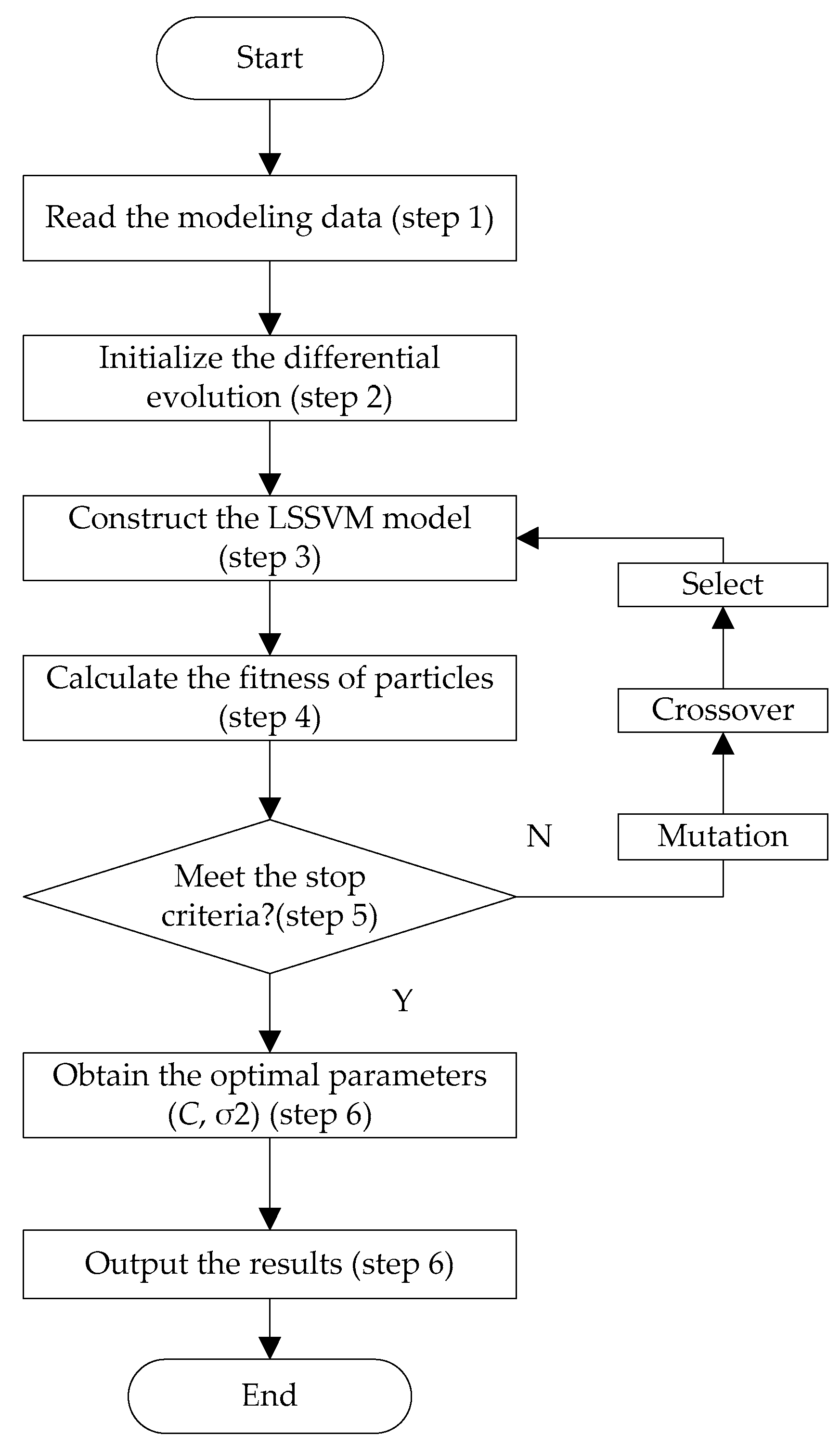
3.3. Construction of the Predictive Model
3.4. Model Validation and Analysis
3.4.1. Experiment Setup
3.4.2. The Model Performance Evaluation Indicators
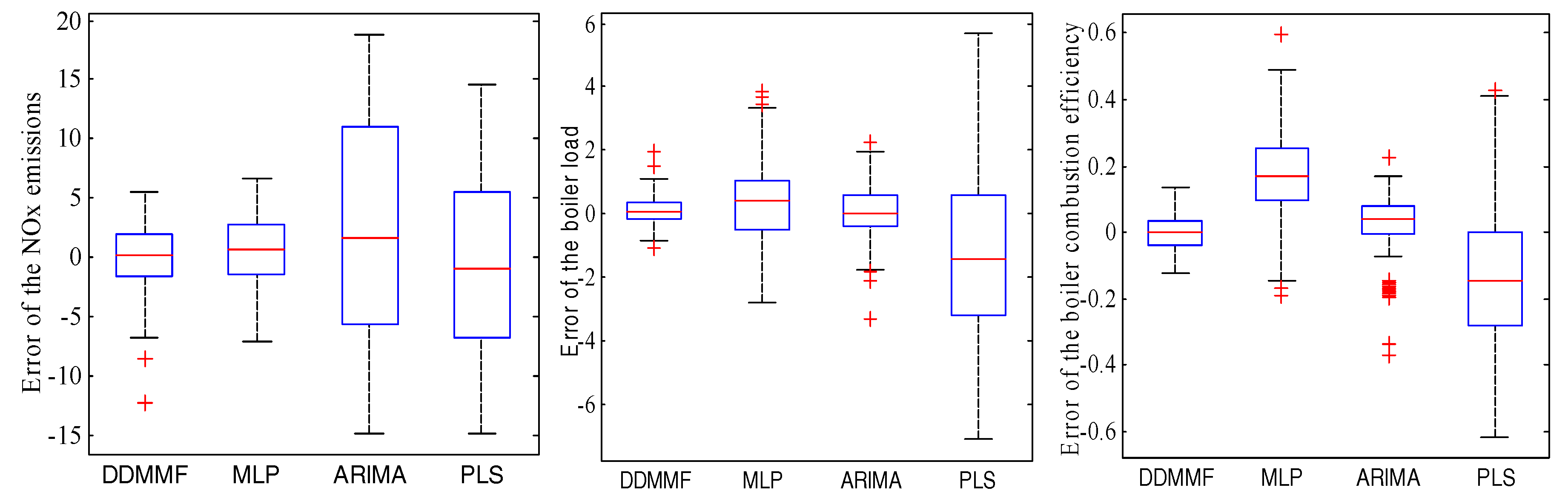
3.4.3. Experimental Result Analysis
4. Adaptive Nonlinear Model Predictive Control of the Boiler Combustion Efficiency
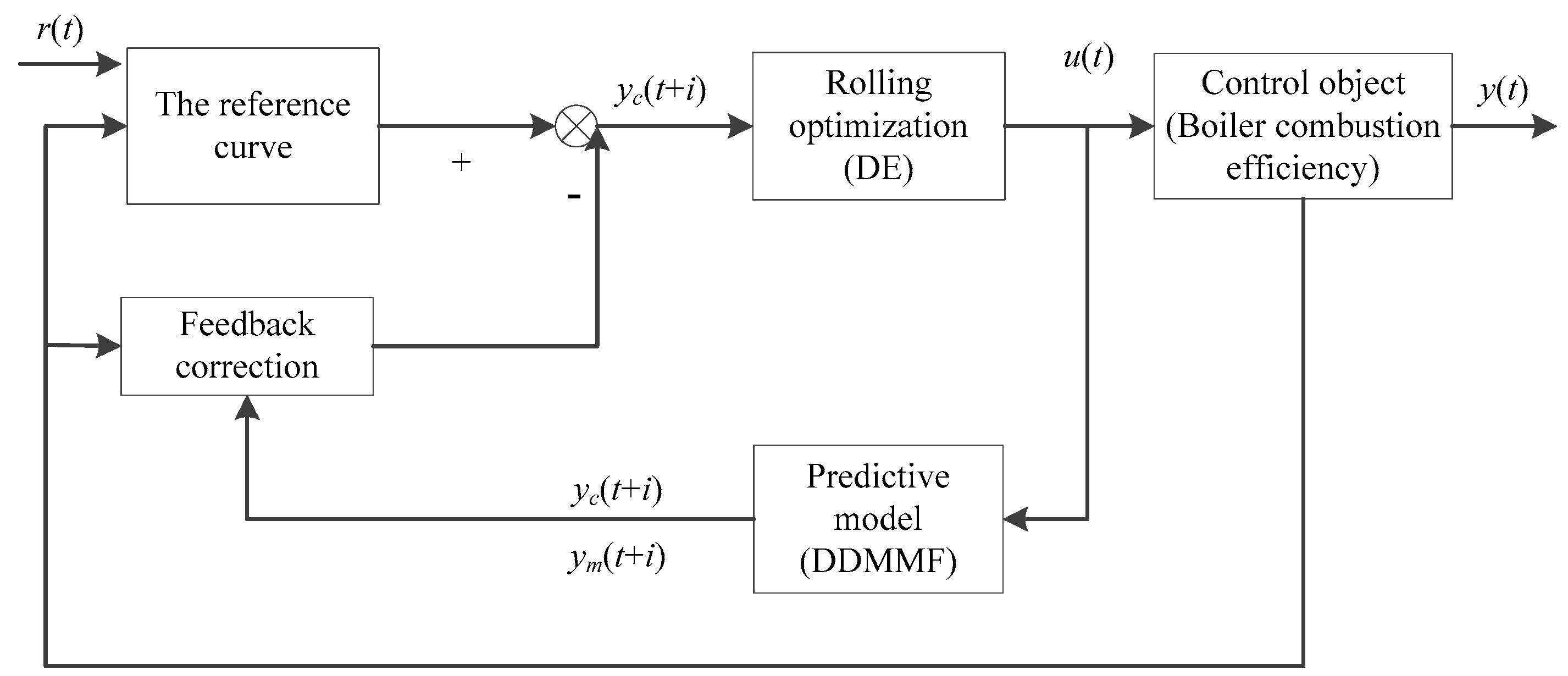
4.1. The Structure of the Proposed Model Predictive Controller
4.2. Rolling Optimization
4.3. Feedback Correction
4.4. Validation of the Model Predictive Control Results
4.4.1. Experiment Setup
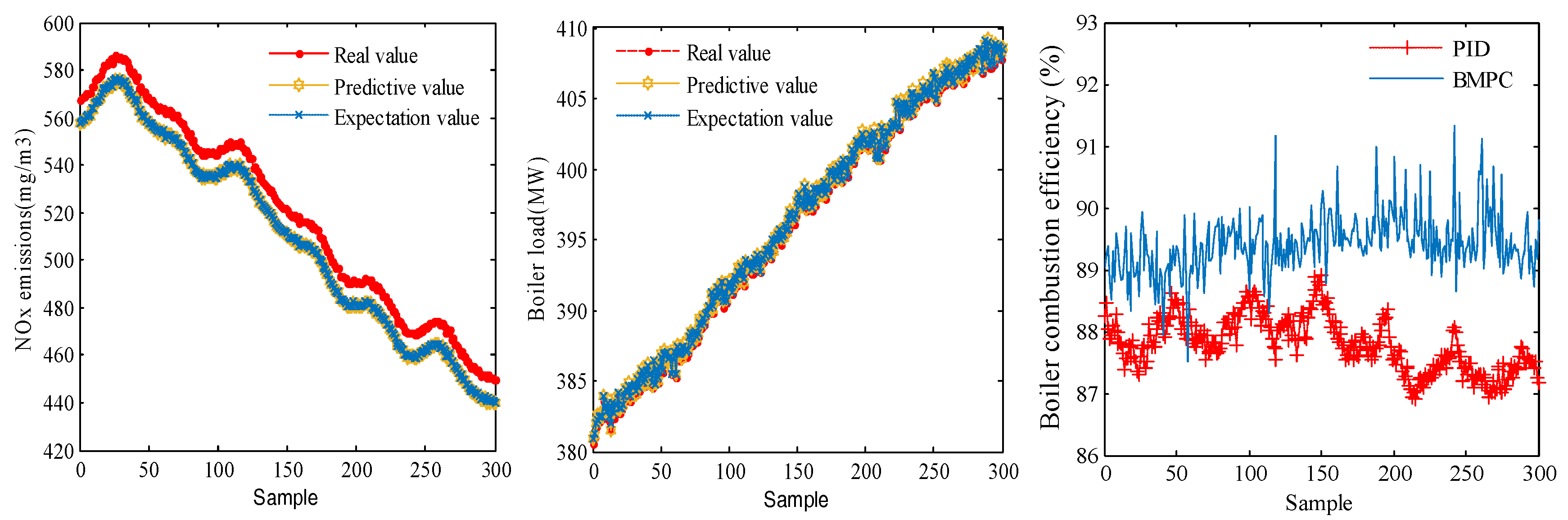
4.4.2. Experimental Result Analysis
5. Conclusions
Author Contributions
Funding
Conflicts of Interest
Acronyms
| NOx | Nitrogen Oxides | CFD | Computational fluid dynamics |
| ARIMA | Autoregressive integrated moving average | PLS | Partial least squares |
| ANN | Artificial neural networking | BP | Back-propagation |
| MLP | Multilayer perceptron | LSSVM | Least square support vector machine; |
| DE | Differential evolution | SIS | Supervisor information system |
| DCS | Distribution control system | PCA | Principal component analysis |
| KNN | Kth Nearest Neighbor | PSO | Particle swarm optimization |
| GA | Genetic algorithm | ADRC | Active disturbance rejection controller |
| MFC-VRFT | Model-Free control and virtual reference feedback tuning | MPC | Model predictive control |
| B | Boiler efficiency | L | Boiler load |
| Nx | NOx emissions | DELSSVM | DE-based LSSVM |
| MAE | Mean absolute error | MAE | Mean absolute error |
| RMSE | Root mean square error | MAPE | Mean absolute percentage error |
| DDMMF | A data-driven modeling method with feature selection capability | BMPC | Model predictive controller |
| PID | Proportion-integral-derivative | RBF | Radial based function |
References
- Ławryńczuk, M. Nonlinear predictive control of a boiler-turbine unit: A state-space approach with successive on-line model linearisation and quadratic optimisation. ISA Trans. 2017, 67, 475–495. [Google Scholar] [CrossRef] [PubMed]
- Zhou, H.; Zheng, L.; Cen, K. Computational intelligence approach for NOx emissions minimizationin a coal-fired utility boiler. Energy Convers. Manag. 2010, 51, 580–586. [Google Scholar] [CrossRef]
- Li, K.; Thompson, S.; Peng, J.X. Modeling and prediction of NOx emission in a coal-fired power generation plant. Control Eng. Pract. 2004, 12, 707–723. [Google Scholar] [CrossRef]
- Gao, Y.; Zeng, D.; Liu, J.; Jian, Y. Optimization control of a pulverizing system on the basis of the estimation of the outlet coal powder flow of a coal mill. Control Eng. Pract. 2017, 63, 69–80. [Google Scholar] [CrossRef]
- Ma, J.; Xu, F.; Huang, K.; Huang, R. Improvement on the linear and nonlinear auto-regressive model for predicting the NOx emission of diesel engine. Neurocomputing 2016, 207, 150–164. [Google Scholar] [CrossRef]
- Fan, H.; Zhang, Y.; Su, Z.; Wang, B. A dynamic mathematical model of an ultra-supercritical coal fired once-through boiler-turbine unit. Appl. Energy 2017, 189, 654–666. [Google Scholar] [CrossRef]
- Kim, B.S.; Kim, T.Y.; Park, T.C.; Yeo, Y.K. Comparative study of estimation methods of NOx emission with selection of input parameters for a coal-fired boiler. Korean J. Chem. Eng. 2018, 35, 1779–1790. [Google Scholar] [CrossRef]
- Strušnik, D.; Golob, M.; Avsec, J. Artificial neural networking model for the prediction of high efficiency boiler steam generation and distribution. Simul. Model. Pract. Theory 2015, 57, 58–70. [Google Scholar] [CrossRef]
- Yin, L.B.; Liu, G.C.; Zhou, J.L.; Liao, Y.F.; Ma, X.Q. A calculation method for CO2 emission in utility boilers based on BP neural network and carbon balance. Energy Procedia 2017, 105, 3173–3178. [Google Scholar] [CrossRef]
- Liukkonen, M.; Hälikkä, E.; Hiltunen, T.; Hiltunen, Y. Dynamic soft sensors for NOx emissions in a circulating fluidized bed boiler. Appl. Energy 2012, 97, 483–490. [Google Scholar] [CrossRef]
- Lv, Y.; Liu, J.; Yang, T.; Zeng, D. A novel least squares support vector machine ensemble model for NOx emission prediction of a coal-fired boiler. Energy 2013, 55, 319–329. [Google Scholar] [CrossRef]
- Lv, Y.; Yang, T.; Liu, J. An adaptive least squares support vector machine model with a novel update for NOx emission prediction. Chemom. Intell. Lab. Syst. 2015, 145, 103–113. [Google Scholar] [CrossRef]
- Xu, C.; Gao, S.; Li, M. A novel PCA-based microstructure descriptor for heterogeneous material design. Comput. Mater. Sci. 2017, 130, 39–49. [Google Scholar] [CrossRef]
- He, F.; Zhang, L. Prediction model of end-point phosphorus content in BOF steelmaking process based on PCA and BP neural network. J. Process Control 2018, 66, 51–58. [Google Scholar] [CrossRef]
- Sayed, M.; Gharghory, S.M.; Kamal, H.A. Gain tuning PI controllers for boiler turbine unit using a new hybrid jump PSO. J. Electr. Syst. Inf. Technol. 2015, 2, 99–110. [Google Scholar] [CrossRef]
- Anarghya, A.; Rao, N.; Nayak, N.; Tirpude, A.R.; Harshith, D.N.; Samarth, B.R. Optimized ANN-GA and experimental analysis of the performance and combustion characteristics of HCCI engine. Appl. Eng. 2018, 132, 841–868. [Google Scholar] [CrossRef]
- Han, J.; Wang, H.F.; Jiao, G.T.; Cui, L.M.; Wang, Y.R. Research on active disturbance rejection control technology of electromechanical actuators. Electronics 2018, 7, 174. [Google Scholar] [CrossRef]
- Roman, R.C.; Radac, M.B.; Precup, R.E.; Pertriu, E.M. Virtual reference feedback tuning of model-Free control algorithms for servo systems. Machinces 2018, 5, 25. [Google Scholar] [CrossRef]
- Pan, Q.K.; Suganthan, P.N.; Wang, L.; Gao, L.; Mallipeddi, R. A differential evolution algorithm with self-adapting strategy and control parameters. Comput. Oper. Res. 2011, 38, 394–408. [Google Scholar] [CrossRef]
- Yu, X.; Yu, X.; Lu, Y.; Yen, G.G.; Cai, M. Differential evolution mutation operators for constrained multi-objective optimization. Appl. Soft Comput. 2018, 67, 452–466. [Google Scholar] [CrossRef]
- Afram, A.; Janabi-Sharifi, F. Supervisory model predictive controller (MPC) for residential HVAC systems: Implementation and experimentation on archetype sustainable house in Toronto. Energy Build. 2017, 154, 268–282. [Google Scholar] [CrossRef]
- Balram, P.; Tuan, L.A.; Carlson, O. Comparative study of MPC based coordinated voltage control in LV distribution systems with photovoltaics and battery storage. Electr. Power Energy Syst. 2018, 95, 227–238. [Google Scholar] [CrossRef]


| Name | Nomenclature | Symbol | Unit | Classical | |
|---|---|---|---|---|---|
| Input variable | Controllable variable | Coal feed | Fc | t/h | B/L/Nx |
| Main feed-water flow | M | t/h | B/L/Nx | ||
| Coal mill inlet airflow A | A1 | t/h | B/L/Nx | ||
| Coal mill inlet airflow B | A2 | t/h | B/L/Nx | ||
| Coal mill inlet airflow C | A3 | t/h | B/L/Nx | ||
| Coal mill inlet airflow D | A4 | t/h | B/L/Nx | ||
| Primary air flow | Pa | t/h | B/L/Nx | ||
| Secondary air flow | S | t/h | B/L/Nx | ||
| State variable | The flue gas oxygen content A | O1 | % | B/Nx | |
| The flue gas oxygen content B | O2 | % | B/Nx | ||
| Coal mill inlet temperature A | T1 | °C | B | ||
| Coal mill inlet temperature B | T2 | °C | B/Nx | ||
| Coal mill inlet temperature C | T3 | °C | B | ||
| Coal mill inlet temperature D | T4 | °C | B/Nx | ||
| Furnace pressure | P | Pa | B | ||
| Output variable | NOx emissions in flue gas | Nx | mg/m3 | ||
| Boiler combustion efficiency | B | % | |||
| Boiler load | L | MW | |||
| Parameter | Number (Condition 1) | Number (Condition 2) | ||||
|---|---|---|---|---|---|---|
| Nx | B | L | Nx | B | L | |
| Train data (samples) | 800 | 800 | 800 | 600 | 600 | 600 |
| Test data (samples) | 300 | 300 | 300 | 270 | 270 | 270 |
| Sample Interval (min) | 1 | 1 | 1 | 1 | 1 | 1 |
| Input variable | 13 | 16 | 9 | 13 | 16 | 9 |
| Output variable | 1 | 1 | 1 | 1 | 1 | 1 |
| Metric | Definition | Equation |
|---|---|---|
| MAE | Mean absolute error | |
| MAPE | Mean absolute percentage error | |
| RMSE | Root mean square error |
| NOx Emissions | Boiler Load | Boiler Efficiency | |||||||
|---|---|---|---|---|---|---|---|---|---|
| Model | MAE (mg/m3) | RMSE (mg/m3) | MARE (%) | MAE (MW) | RMSE (MW) | MARE (%) | MAE (%) | RMSE (%) | MARE (%) |
| DDMMF | 1.697 | 13.466 | 4.9 × 10⁻⁴ | 0.001 | 4.244 | 0.001 | 0.010 | 0.162 | 7.3 × 10⁻⁵ |
| MLP | 1.766 | 14.138 | 9.4 × 10⁻⁴ | 0.029 | 11.567 | 0.011 | 0.058 | 0.184 | 2.0 × 10⁻⁴ |
| ARIMA | 2.559 | 28.249 | 1.9 × 10⁻³ | 3.520 | 21.563 | 0.789 | 0.040 | 0.712 | 5.1 × 10⁻⁴ |
| PLS | 2.321 | 15.844 | 3.0 × 10⁻³ | 0.963 | 35.940 | 0.631 | 0.118 | 1.628 | 2.8 × 10⁻⁴ |
| NOx Emissions | Boiler Load | Boiler Efficiency | |||||||
|---|---|---|---|---|---|---|---|---|---|
| Model | MAE (mg/m3) | RMSE (mg/m3) | MARE (%) | MAE (MW) | RMSE (MW) | MARE (%) | MAE (%) | RMSE (%) | MARE (%) |
| DDMMF | 1.518 | 1.674 | 0.329 | 0.519 | 1.789 | 0.003 | 0.021 | 0.474 | 1.5 × 10⁻⁴ |
| MLP | 1.883 | 7.832 | 1.899 | 4.683 | 6.649 | 0.012 | 0.149 | 2.975 | 8.4 × 10⁻⁴ |
| ARIMA | 5.405 | 15.062 | 1.054 | 0.001 | 6.634 | 0.005 | 0.128 | 0.981 | 3.7 × 10⁻⁴ |
| PLS | 2.321 | 16.946 | 2.443 | 0.115 | 4.630 | 0.005 | 0.065 | 0.684 | 5.4 × 10⁻⁴ |
| Parameter | Number (Condition 1) | Number (Condition 2) | ||||
|---|---|---|---|---|---|---|
| Nx | B | L | Nx | B | L | |
| Test data (samples) | 300 | 300 | 300 | 270 | 270 | 270 |
| Sample Interval (min) | 1 | 1 | 1 | 1 | 1 | 1 |
| Input variable | 13 | 16 | 9 | 13 | 16 | 9 |
| Output variable | 1 | 1 | 1 | 1 | 1 | 1 |
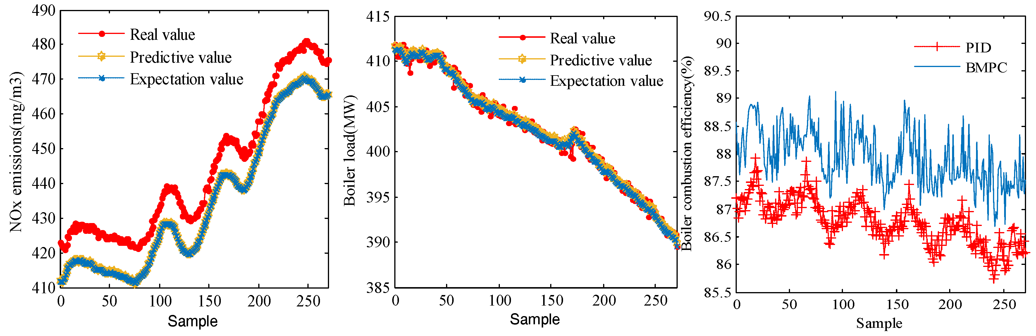
| Description | The Predictive Control Error of NOx Emissions / Boiler Load (%) | The Percentage of NOx Emissions Decline by BMPC | The Percentage of Boiler Efficiency Improvement by BMPC | Number of Samples |
|---|---|---|---|---|
| the operation condition 1 | −4.911~4.969 | 1.887 | 1.613 | 300 |
| the operation condition 2 | −4.989~4.995 | 2.166 | 1.136 | 270 |
© 2019 by the authors. Licensee MDPI, Basel, Switzerland. This article is an open access article distributed under the terms and conditions of the Creative Commons Attribution (CC BY) license (http://creativecommons.org/licenses/by/4.0/).
Share and Cite
Tang, Z.; Wu, X.; Cao, S. Adaptive Nonlinear Model Predictive Control of the Combustion Efficiency under the NOx Emissions and Load Constraints. Energies 2019, 12, 1738. https://doi.org/10.3390/en12091738
Tang Z, Wu X, Cao S. Adaptive Nonlinear Model Predictive Control of the Combustion Efficiency under the NOx Emissions and Load Constraints. Energies. 2019; 12(9):1738. https://doi.org/10.3390/en12091738
Chicago/Turabian StyleTang, Zhenhao, Xiaoyan Wu, and Shengxian Cao. 2019. "Adaptive Nonlinear Model Predictive Control of the Combustion Efficiency under the NOx Emissions and Load Constraints" Energies 12, no. 9: 1738. https://doi.org/10.3390/en12091738
APA StyleTang, Z., Wu, X., & Cao, S. (2019). Adaptive Nonlinear Model Predictive Control of the Combustion Efficiency under the NOx Emissions and Load Constraints. Energies, 12(9), 1738. https://doi.org/10.3390/en12091738