Sensors Fault Diagnosis and Active Fault-Tolerant Control for PMSM Drive Systems Based on a Composite Sliding Mode Observer

Abstract

Due to the use of multiple observers and controllers in multi-sensor fault-tolerant control of PMSM drive systems, the algorithm is complex and the system control performance is affected. In view of this, the paper studies multi-sensor fault diagnosis and active fault-tolerant control strategies based on a composite sliding mode observer. With the mathematical model of PMSM built, a design method of the composite sliding mode observer is proposed. A single observer is used to observe and estimate various state variables in the system in real time, which simplifies the implementation of observer-related algorithms. In order to improve the diagnostic accuracy of different types of sensors under different faults, a method for determining fault thresholds is proposed through global search for the maximum residual value. Based on this, a fault diagnosis and active fault-tolerant control strategy is proposed to realize fast switching and reconstruction of feedback signals of closed-loop control systems under different faults of multiple sensors, thus restoring the system performance. Finally, the effectiveness of the proposed algorithm and control strategy is verified by simulation experiments

1. Introduction

With the increasing use of electric vehicles worldwide, the industry’s technical requirements for its core component—the electric drive system—continue to increase [1]. In recent years, the Permanent Magnet Synchronous Motor (PMSM) concept has attracted more and more attention in electric vehicle applications due to its high density, great efficiency, small size, light weight, and low cost [2,3]. The corresponding technologies of the PMSM drive system have become a research hotspot among scholars at home and abroad. Generally, the PMSM drive system is equipped with current, speed and position sensors to obtain the feedback signals of three-phase stator current, motor speed and position, which are required for the closed-loop control operation of the system. Obviously, the normal operation of various types of sensors is a basic guarantee to achieve stable and reliable operation of the PMSM drive system. However, due to the increasingly complex working environment, aging of devices and external interference, the sensors in the system are prone to failure, resulting in deviations in the feedback signals of the control system, which in turn affects the control performance and, in severe cases, even causes damage to other electrical equipment. Therefore, the fault diagnosis and fault-tolerance control of sensors in the PMSM drive system of electric vehicles are of great importance.

At present, the methods for sensor fault diagnosis and fault-tolerant control of PMSM drive systems can be divided into two categories: data-driven methods and analytical model-based methods. Data-driven methods do not require the establishment of accurate mathematical models. However, large amounts of data are needed to obtain prior knowledge so as to achieve fault diagnosis through data analysis. Data-driven methods have good diagnostic effect on sensor faults, but can hardly provide reliable fault-tolerant control [4,5]. Analytical model-based methods mainly establish a mathematical analytic model based on the operating state of system, and construct residuals and other physical signals for fault diagnosis and fault-tolerant control. The three main methods are as follows: (1) The current reconstruction method [6,7,8]. This method estimates the current by reconstructing space vectors to achieve sensor fault diagnosis and fault-tolerant control. Though it is simple and satisfies the requirements of corresponding systems for stable operation under current sensor fault, it cannot be applied universally due to the great difference in the current reconstruction methods of different systems. (2) The Luenberger-based observer method [9,10,11]. In this method, the establishment of the Luenberger observer can solve the universality problem effectively, but the observer is highly susceptible to the influence of parameter changes and external disturbances, which may even cause misdiagnosis or missed diagnosis. (3) The sliding mode observer-based method [12,13]. The sliding mode observer has stronger robustness and anti-disturbance than the Luenberger observer and can improve the diagnostic accuracy of the system, but its mathematical model is often complicated due to the high electromagnetic coupling of the motor drive system.

The above methods are widely used in fault diagnosis and fault-tolerant control of a single sensor in PMSM drive system, and have achieved good results. In the actual system, faults may occur to all kinds of sensors, so considering the faults of a single sensor alone cannot guarantee the stable operation of the system. Hence, the fault-tolerant control for multiple types of sensor faults is particularly important. Currently, research mainly focuses on the establishment of multiple observers based on analytical model methods to realize multi-sensor fault diagnosis and fault-tolerant control of PMSM drive system [14,15]. Among them, [14] comprehensively considered the faults in three types of sensors: DC side voltage sensor, AC side current sensor and motor speed sensor of the PMSM drive system. Two high-order sliding mode observers and one Luenberger observer were designed, in which the high-order sliding mode observers estimated the system voltage and speed, respectively, while the Luenberger observer estimated the system current. The three observers operated in parallel so as to realize diagnosis and fault-tolerant control of the voltage, current and speed sensor faults of the PMSM drive system. Though it enhanced the robust performance of the system, the integral effect of the high-order sliding mode had an impact on the fast response characteristics of the system. Ref. [15] also designed the self-adaptive observer, Luenberger observer and speed sensorless observer for the three types of sensors to estimate the corresponding voltage, current and speed. High frequency signals were injected into the low speed interval to improve the system performance. The diagnosis and fault tolerance control was relatively fast, as there was no integral term. However, both [14] and [15] required multiple observers to operate at the same time, which not only complicated the algorithm but also increased the time cost of the system. Also, multiple observers often interacted with each other when operating in parallel, thus reducing the overall system performance. On the other hand, for the PMSM drive system, the establishment of multiple observers will reduce the sensitivity of the various components of the system and the overall reliability of the system to a certain extent [16], which affects the accuracy of fault diagnosis and the effectiveness of fault-tolerant control.

In summary, accurate diagnosis of sensor faults in PMSM drive systems is the basic premise for fault-tolerant control. In the process of fault diagnosis based on an observer, the selection of the threshold of each observation variable affects the accuracy of the sensor fault diagnosis directly. If the threshold is too small, when there is noise interference in the system or the model is biased, not only will misdiagnosis occur but also faulty fault-tolerant control will be triggered, which will cause safety problems for the PMSM system. On the contrary, if the threshold is too large, there will be a possibility of missed diagnosis, which increases the security risk of the system as well. At present, there are three main methods to set the thresholds for sensor fault diagnosis of PMSM drive system: (1) By observing the difference of residuals [17]. This method only considers the single influence of the observation errors, so the overall diagnostic accuracy of the system is low. (2) By considering noise [12]. The observation errors and measurement noise are both taken into consideration to minimize misdiagnosis rate and improve fault detection efficiency. (3) By considering parameter variations [14]. This method further considers the influence of system parameter variations on the basis of observation errors and measurement noise, so the diagnostic accuracy can be further improved. However, in actual operation, the permanent magnet of the PMSM is prone to demagnetization due to the influence of temperature, mechanical action, and armature reaction magnetic field, which affects the residual values of observed variables [18]. If the demagnetization is not considered when setting the threshold, it is very likely that misdiagnosis will occur.

In view of the multi-sensor fault problems, a composite sliding mode observer is designed in this paper based on the double closed-loop current and speed control strategy of the PMSM control system [19]. A single observer is used to observe and estimate the various state variables in real time, which simplifies not only the implementation of the observer-related algorithm but also the sensor fault diagnosis and isolation control algorithm. Meanwhile, in order to improve the diagnostic accuracy of system under multi-sensor faults, a method for determining the fault thresholds is proposed through global search for the maximum residual value. Based on this, a fault diagnosis and active fault-tolerant control strategy is proposed to realize fast switching and reconstruction of feedback signals of closed-loop control systems under different faults of multiple sensors, thus restoring the system performance. Finally, the effectiveness of the proposed algorithm and control strategy is verified by simulating the occurrence of different faults of the three types of sensors.

2. Overall Control Process of the Proposed Fault Diagnosis and Active Fault-Tolerant Control System

During normal operation, the PMSM drive system requires current, speed and position sensors [20], in which the position sensor is difficult to install due to its large size and high cost. It also increases the moment of inertia of the bearing and affects the dynamic and steady-state characteristics and robustness of the system. In recent years, some scholars have developed sensorless motor position control technologies based on indirect detection of the rotor position [21,22], which have found wide applications. With low cost and easy implementation in mind and on the basis of the traditional PMSM control system based on current and speed double closed-loop, this paper designs a composite sliding mode observer to observe and estimate multiple variables of the system. Studies are conducted on the fault diagnosis and active fault-tolerant control of the three-phase current sensors and motor speed sensor of the PMSM drive system.

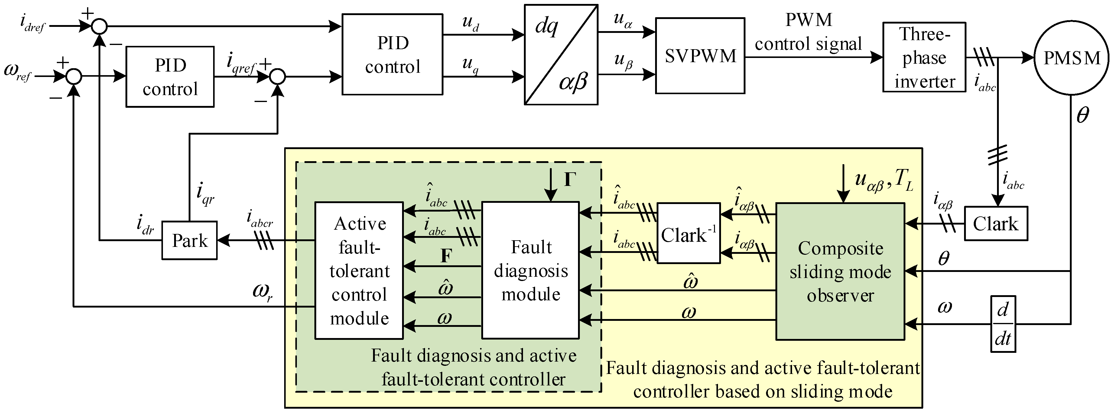
As shown in Figure 1, among the fault diagnosis and active fault-tolerant control system, the fault diagnosis and active fault-tolerant controller based on sliding mode mainly includes two parts: a composite sliding mode observer and a fault diagnosis and active fault-tolerant controller. The corresponding fault-tolerant control is as follows: (1) Establish the fault thresholds of the system-related variables Γ = [Γ_ia Γ_ib Γ_ic Γ_ω]^T offline. 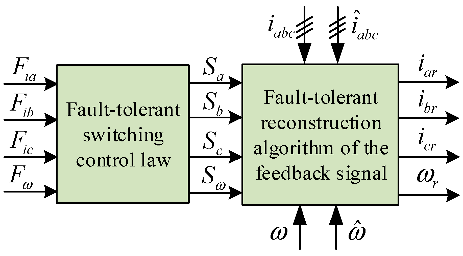Store the values in the fault diagnosis module, including the three-phase current thresholds Γ_ia, Γ_ib, Γ_ic and the speed threshold Γ_ω. (2) During system operation, the composite sliding mode observer estimates, in real time, the three-phase current and speed signals in the system, and inputs the corresponding estimated values and the measured values of the sensor altogether into the fault diagnosis module. (3) The fault diagnosis module generates the system residuals in real time according to the estimated values and the measured values of the three-phase current and speed signals, and compares them with the thresholds for fault diagnosis. (4) Based on the fault diagnosis results, the active fault-tolerant control module designs a corresponding algorithm to reconstruct and change the current and speed feedback signals of the original closed-loop control system, thereby eliminating the influence of the faulty sensor and achieving active fault-tolerant control under sensor fault.

The following sections will design a composite sliding mode observer as well as a fault diagnosis and active fault-tolerant controller based on the established PMSM mathematical model to realize fault diagnosis and active fault-tolerant control of sensors in the PMSM drive system.

3. The Design of Composite Sliding Mode Observer

3.1. PMSM Mathematical Model

The mathematical model of PMSM in an α − β two-phase stationary coordinate system includes stator voltage equation, stator flux linkage equation, electromagnetic torque equation and motion Equation [23].

The corresponding stator voltage equation is:

$$\{\begin{array}{l}{u}_{\alpha }=R_s{i}_{\alpha }+L_s\frac{d{i}_{\alpha }}{dt}-\omega {\psi }_{\mathrm{f}}\sin \theta \\ u_{\beta }=R_s{i}_{\beta }+L_s\frac{d{i}_{\beta }}{dt}+\omega {\psi }_{\mathrm{f}}\cos \theta \end{array}$$

(1)

The stator flux linkage equation is:

$$\{\begin{array}{l}{\psi }_{\alpha }={\displaystyle \int (u_{\alpha }-R_s{i}_{\alpha })dt}\\ {\psi }_{\beta }={\displaystyle \int (u_{\beta }-R_s{i}_{\beta })dt}\end{array}$$

(2)

The electromagnetic torque equation is:

$$T_e=\frac{3}{2}{n}_p({\psi }_{\alpha }{i}_{\beta }-{\psi }_{\beta }{i}_{\alpha })$$

(3)

The motion equation is:

$$T_e-T_L=\frac{J}{n_p}\frac{d\omega }{dt}$$

(4)

In the above equations, u_α and u_β are stator voltages, i_α and i_β are stator currents, ψ_α and ψ_β are stator fluxes, R_s and L_s are stator resistance and inductance, respectively, ω is the rotor angular velocity, θ is the rotor position angle, ψ_f is the rotor permanent magnet flux, T_e is the electromagnetic torque, T_L is the load torque, n_p is the pole pair of the motor, and J is the moment of inertia.

From Equations (1)–(4), we obtain:

$$\{\begin{array}{l}\frac{d{i}_{\alpha }}{dt}=-\frac{R_s}{L_s}{i}_{\alpha }+\frac{1}{L_s}{\psi }_{\mathrm{f}}\omega \sin \theta +\frac{1}{L_s}{u}_{\alpha }\\ \frac{d{i}_{\beta }}{dt}=-\frac{R_s}{L_s}{i}_{\beta }-\frac{1}{L_s}{\psi }_{\mathrm{f}}\omega \cos \theta +\frac{1}{L_s}{u}_{\beta }\\ \frac{d\omega }{dt}=-\frac{3n_p^2}{2J}{\psi }_{\mathrm{f}}{i}_{\alpha }\sin \theta +\frac{3n_p^2}{2J}{\psi }_{\mathrm{f}}{i}_{\beta }\cos \theta -\frac{n_p}{J}{T}_L\end{array}$$

(5)

Meanwhile, the relationship between the stator currents and voltages in the abc three-phase coordinate system and the stator currents and voltages in the α − β two-phase coordinate system is as follows:

$$\left(\begin{array}{c}{i}_a\\ i_b\\ i_c\end{array}\right)=\left(\begin{array}{cc}1& 0\\ -1/2& \sqrt{3}/2\\ -1/2& -\sqrt{3}/2\end{array}\right)\left(\begin{array}{c}{i}_{\alpha }\\ i_{\beta }\end{array}\right),\left(\begin{array}{c}{u}_a\\ u_b\\ u_c\end{array}\right)=\left(\begin{array}{cc}1& 0\\ -1/2& \sqrt{3}/2\\ -1/2& -\sqrt{3}/2\end{array}\right)\left(\begin{array}{c}{u}_{\alpha }\\ u_{\beta }\end{array}\right)$$

(6)

where u_a, u_b and u_c are the stator voltages in the three-phase coordinate system, and i_a, i_b and i_c are the stator currents in the three-phase coordinate system.

Then, we have the state space model [24] of the PMSM drive system.

$$\{\begin{array}{l}\dot{\mathbf{x}}=\mathbf{Ax}+\mathbf{Bu}\\ \mathbf{y}=\mathbf{Cx}\end{array}$$

(7)

where x = [i_α i_β ω]^T is the state variable, u = [u_α u_β T_L]^T is the input vector, y = [ω] is the output vector, and the coefficient matrixes are:

$$\mathbf{A}=\left[\begin{array}{ccc}-\frac{R_s}{L_s}& 0& \frac{1}{L_s}{\psi }_{\mathrm{f}}\sin \theta \\ 0& -\frac{R_s}{L_s}& -\frac{1}{L_s}{\psi }_{\mathrm{f}}\cos \theta \\ -\frac{3n_p^2}{2J}{\psi }_{\mathrm{f}}\sin \theta & \frac{3n_p^2}{2J}{\psi }_{\mathrm{f}}\cos \theta & 0\end{array}\right],\mathbf{B}=\left[\begin{array}{ccc}\frac{1}{L_s}& 0& 0\\ 0& \frac{1}{L_s}& 0\\ 0& 0& -\frac{n_p}{J}\end{array}\right],\mathbf{C}=\left[\begin{array}{ccc}0& 0& 1\end{array}\right].$$

3.2. Composite Sliding Mode Observer Design

According to the state space model of PMSM in the α − β two-phase stationary coordinate system, the composite sliding mode observer is constructed as:

$$\{\begin{array}{l}\dot{\widehat{\mathbf{x}}}=\mathbf{A}\widehat{\mathbf{x}}+\mathbf{Bu}+{\mathbf{G}}_n\mathbf{v}\\ \widehat{\mathbf{y}}=\mathbf{C}\widehat{\mathbf{x}}\end{array}$$

(8)

where $\widehat{\mathbf{x}}=[{\widehat{i}}_{\mathbf{\alpha }}{\widehat{i}}_{\beta }\widehat{\omega }{]}^T$, $\widehat{\mathbf{y}}=\left[\widehat{\omega }\right]$, ${\widehat{i}}_{\mathbf{\alpha }},{\widehat{i}}_{\beta }$ and $\widehat{\omega }$ are the estimated values of i_α, i_β and ω, respectively, v is a nonlinear discontinuous term, and G_n is a gain matrix.

Suppose that the system state estimation error is defined as:

$$\mathbf{e}=\left[\begin{array}{c}{e}_{i\alpha }\\ e_{i\beta }\\ e_{\omega }\end{array}\right]=\widehat{\mathbf{x}}-\mathbf{x}=\left[\begin{array}{c}{\widehat{i}}_{\alpha }-i_{\alpha }\\ {\widehat{i}}_{\beta }-i_{\beta }\\ \widehat{\omega }-\omega \end{array}\right]$$

(9)

The system output estimation error is defined as:

$${\mathbf{e}}_y=[e_{\omega }]=\widehat{\mathbf{y}}-\mathbf{y}=\left[\widehat{\omega }-\omega \right]$$

(10)

Then, for a composite sliding mode observer, the sliding mode surface is designed as:

$$\mathbf{s}=\mathbf{e}=\left[\begin{array}{c}{e}_{i\alpha }\\ e_{i\beta }\\ e_{\omega }\end{array}\right]=\left[\begin{array}{c}{\widehat{i}}_{\alpha }-i_{\alpha }\\ {\widehat{i}}_{\beta }-i_{\beta }\\ \widehat{\omega }-\omega \end{array}\right]$$

(11)

The nonlinear discontinuous high-frequency switching term v is likely to cause system chattering [25], thus increasing the computational burden. Therefore, the discontinuity of v should be “smoothed” to avoid or alleviate system chattering. In order to make the system state variables approximate the sliding mode surface, this paper uses the sigmoid function to define the approximate smoothing term as:

$$\mathbf{v}={\left[\begin{array}{ccc}\rho (\frac{2}{1-2e^{e_{i\alpha }}}-1)& \rho (\frac{2}{1-2e^{e_{i\beta }}}-1)& \rho (\frac{2}{1-2e^{e_{\omega }}}-1)\end{array}\right]}^T$$

(12)

where ρ is a positive real scalar.

Suppose that the gain matrix G_n has the following structure, namely, G_n = diag(g₁,g₂,−1), g₁,g₂ ∈ R. From Equations (5), (8), (11), and (12), we can obtain ${\widehat{i}}_{\mathbf{\alpha }},{\widehat{i}}_{\beta }$ and $\widehat{\omega }$ in the system:

$$\begin{array}{l}\left[\begin{array}{c}{\dot{\widehat{i}}}_{\alpha }\\ {\dot{\widehat{i}}}_{\beta }\\ \dot{\widehat{\omega }}\end{array}\right]=\left[\begin{array}{ccc}-\frac{R_s}{L_s}& 0& \frac{1}{L_s}{\psi }_{\mathrm{f}}\sin \theta \\ 0& -\frac{R_s}{L_s}& -\frac{1}{L_s}{\psi }_{\mathrm{f}}\cos \theta \\ -\frac{3n_p^2}{2J}{\psi }_{\mathrm{f}}\sin \theta & \frac{3n_p^2}{2J}{\psi }_{\mathrm{f}}\cos \theta & 0\end{array}\right]\left[\begin{array}{c}{\widehat{i}}_{\alpha }\\ {\widehat{i}}_{\beta }\\ \widehat{\omega }\end{array}\right]\\ +\left[\begin{array}{ccc}\frac{1}{L_s}& 0& 0\\ 0& \frac{1}{L_s}& 0\\ 0& 0& -\frac{n_p}{J}\end{array}\right]\left[\begin{array}{c}{u}_{\alpha }\\ u_{\beta }\\ T_L\end{array}\right]+\left[\begin{array}{ccc}{g}_1& 0& 0\\ 0& g_2& 0\\ 0& 0& -1\end{array}\right]\left[\begin{array}{c}\rho (\frac{2}{1-2e^{e_{i\alpha }}}-1)\\ \rho (\frac{2}{1-2e^{e_{i\beta }}}-1)\\ \rho (\frac{2}{1-2e^{e_{\omega }}}-1)\end{array}\right]\end{array}$$

(13)

With the above equation, the stator currents and speed of the motor can be observed and estimated in real time, paving the way for subsequent fault diagnosis and active fault-tolerant control. It can be proved that the sliding mode observer designed based on the above method is stable and feasible, and the corresponding gain matrix G_n and the positive scalar ρ can be derived. What follows is the proof and the specific derivation process.

According to the structure of the coefficient matrix C in the composite sliding mode observer, the system state estimation error defined by Equation (9) can be further broken into e = [e₁ e_y]^T, e₁ ∈ R^2×1. Meanwhile, the Lyapunov function is defined as V = 1/2e^Te.

In order for the system to reach the sliding mode surface within a limited time from any initial state, it must satisfy the condition V^& < 0. Namely:

$$\dot{V}={\left(\frac{1}{2}{\mathbf{e}}^T\mathbf{e}\right)}^{\prime }={\left(\frac{1}{2}\left[\begin{array}{cc}{\mathbf{e}}_1& {\mathbf{e}}_y\end{array}\right]\left[\begin{array}{c}{\mathbf{e}}_1\\ {\mathbf{e}}_y\end{array}\right]\right)}^{\prime }={\left(\frac{1}{2}{\mathbf{e}}_1^2+\frac{1}{2}{\mathbf{e}}_y^2\right)}^{\prime }={\mathbf{e}}_y\cdot {\dot{\mathbf{e}}}_y+{\mathbf{e}}_1\cdot {\dot{\mathbf{e}}}_1<0$$

(14)

To prove $\dot{V}<0$, we can first prove that the following two equations are valid:

$${\dot{V}}_1={\mathbf{e}}_y\cdot {\dot{\mathbf{e}}}_y<0$$

(15)

$${\dot{V}}_2={\mathbf{e}}_1\cdot {\dot{\mathbf{e}}}_1<0$$

(16)

The proof of Equation (15) is as follows:

According to Equations (7) and (8), we have:

$$\dot{\mathbf{e}}=\mathbf{Ae}+{\mathbf{G}}_n\mathbf{v}$$

(17)

It can be broken up into:

$$\{\begin{array}{l}{\dot{\mathbf{e}}}_1={\mathbf{A}}_{11}{\mathbf{e}}_1+{\mathbf{A}}_{12}{\mathbf{e}}_y+{\mathbf{G}}_{n1}{\mathbf{v}}_1\\ {\dot{\mathbf{e}}}_y={\mathbf{A}}_{21}{\mathbf{e}}_1+{\mathbf{A}}_{22}{\mathbf{e}}_y-{\mathbf{v}}_2\end{array}$$

(18)

where ${\mathbf{A}}_{11}=\left[\begin{array}{cc}-\frac{R_s}{L_s}& 0\\ 0& -\frac{R_s}{L_s}\end{array}\right]$, ${\mathbf{A}}_{12}=\left[\begin{array}{c}\frac{1}{L_s}{\psi }_{\mathrm{f}}\sin \theta \\ -\frac{1}{L_s}{\psi }_{\mathrm{f}}\cos \theta \end{array}\right]$, ${\mathbf{A}}_{21}=\left[\begin{array}{cc}-\frac{3n_p^2}{2J}{\psi }_{\mathrm{f}}\sin \theta & \frac{3n_p^2}{2J}{\psi }_{\mathrm{f}}\cos \theta \end{array}\right]$, ${\mathbf{A}}_{22}=\left[0\right]$, ${\mathbf{G}}_{n1}=\left[\begin{array}{cc}{g}_1& 0\\ 0& g_2\end{array}\right]$, ${\mathbf{v}}_1={\left[\begin{array}{cc}\rho (\frac{2}{1-2e^{e_{i\alpha }}}-1)& \rho (\frac{2}{1-2e^{e_{i\beta }}}-1)\end{array}\right]}^T$, ${\mathbf{v}}_2={\left[\rho (\frac{2}{1-2e^{e_{\omega }}}-1)\right]}^T$.

Then:

$${\dot{\mathbf{e}}}_y={\mathbf{A}}_{21}{\mathbf{e}}_1+{\mathbf{A}}_{22}{\mathbf{e}}_y-\rho (\frac{2}{1-2e^{e_{\omega }}}-1)$$

(19)

Multiplying both sides by e_y we have:

$$\begin{array}{ll}{\mathbf{e}}_y\cdot {\dot{\mathbf{e}}}_y& ={\mathbf{e}}_y\cdot ({\mathbf{A}}_{21}{\mathbf{e}}_1+{\mathbf{A}}_{22}{\mathbf{e}}_y-\rho (\frac{2}{1-2e^{e_{\omega }}}-1))\\ & ={\mathbf{e}}_y\cdot ({\mathbf{A}}_{21}{\mathbf{e}}_1+{\mathbf{A}}_{22}{\mathbf{e}}_y)-\rho \left|{\mathbf{e}}_y\right|\\ & <-\left|{\mathbf{e}}_y\right|\cdot (\rho -\left|({\mathbf{A}}_{21}{\mathbf{e}}_1+{\mathbf{A}}_{22}{\mathbf{e}}_y)\right|)\end{array}$$

(20)

When the positive scalar ρ satisfies the following:

$$\rho -\left|{\mathbf{A}}_{21}{\mathbf{e}}_1+{\mathbf{A}}_{22}{\mathbf{e}}_y\right|>\zeta >0$$

(21)

where ζ ∈ R₊, then Equation (15) can be proved, that is, $V_1^{\&}={\mathbf{e}}_y·{\mathbf{e}}_y^{\&}<0$.

The proof of Equation (16) is as follows:

When the positive scalar ρ satisfies Equation (21), and assume that there is no model mismatch or disturbances, the system output estimation error will converge to zero in a finite time. At this point, Equation (18) can be approximated as:

$${\dot{\mathbf{e}}}_1=({\mathbf{A}}_{11}+{\mathbf{G}}_{n1}\left[\begin{array}{c}{\mathbf{A}}_{21}\\ {\mathbf{A}}_{21}\end{array}\right])\cdot {\mathbf{e}}_1$$

(22)

In order to make the system in a stable reduced-order motion when entering the sliding mode [26], it is necessary to ensure that the determinant of coefficient matrix in Equation (22) is less than zero:

$$\begin{array}{ll}\left|{\mathbf{A}}_{11}+{\mathbf{G}}_{n1}\left[\begin{array}{c}{\mathbf{A}}_{21}\\ {\mathbf{A}}_{21}\end{array}\right]\right|& =\left|\left[\begin{array}{cc}-R_s/L_s-3n_p^2{\psi }_{\mathrm{f}}{g}_1\sin \theta /2J& 3n_p^2{\psi }_{\mathrm{f}}{g}_1\cos \theta /2J\\ -3n_p^2{\psi }_{\mathrm{f}}{g}_2\sin \theta /2J& -R_s/L_s+3n_p^2{\psi }_{\mathrm{f}}{g}_2\cos \theta /2J\end{array}\right]\right|\\ & =\frac{R_s^2}{L_s^2}+\frac{3R_s{n}_p^2}{2L_{s}J}{\psi }_{\mathrm{f}}{g}_1\sin \theta -\frac{3R_s{n}_p^2}{2L_{s}J}{\psi }_{\mathrm{f}}{g}_2\cos \theta <0\end{array}$$

(23)

Then, we have:

$${\mathbf{e}}_1\cdot {\dot{\mathbf{e}}}_1=\left|{\mathbf{A}}_{11}+{\mathbf{G}}_{n1}\left[\begin{array}{c}{\mathbf{A}}_{21}\\ {\mathbf{A}}_{21}\end{array}\right]\right|\cdot {\mathbf{e}}_1^2<0$$

(24)

Therefore, when the parameters g₁ and g₂ in the gain matrix G_n satisfy the following equation, Equation (16) can be proved, that is, $V_2^{\&}={\mathbf{e}}_1·{\mathbf{e}}_1^{\&}<0$:

$$g_1\sin \theta -g_2\cos \theta <-\frac{R_{s}J}{L_s{n}_p^2{\psi }_{\mathrm{f}}}$$

(25)

In summary, when the sliding mode observer parameters (g₁ and g₂) and the positive scalar ρ satisfy Equation (26), we have $\dot{V}<0$. Then, the sliding mode observer proposed above is accessible in the state space:

$$\{\begin{array}{l}{g}_1\sin \theta -g_2\cos \theta <-\frac{R_{s}J}{L_s{n}_p^2{\psi }_{\mathrm{f}}}\\ \rho >\left|{\mathbf{A}}_{21}{\mathbf{e}}_1+{\mathbf{A}}_{22}{\mathbf{e}}_y\right|>0\end{array}$$

(26)

3.3. Anti-Disturbance Performance Analysis of the Composite Sliding Mode Observer

From the previous analysis, we know that scholars at home and abroad tend to use the classic Luenberger observer to deal with sensor failures in the motor drive system. By comparison, the composite sliding mode observer proposed in this paper has better anti-disturbance performance. The detailed analysis is given below.

Let the interference signal be ξ(t) and its distribution matrix be Q. Then the state space model described by Equation (7) becomes:

$$\{\begin{array}{l}\dot{\mathbf{x}}(t)=\mathbf{Ax}(t)+\mathbf{Bu}(t)+\mathbf{Q}\xi (t)\\ \mathbf{y}(t)=\mathbf{Cx}(t)\end{array}$$

(27)

The distribution matrix Q matches the gain matrix G_n, and there exists a matrix X which satisfies Equation (28):

$$\mathbf{Q}=\left[\begin{array}{c}{\mathbf{G}}_{n1}\mathbf{X}\\ -\mathbf{X}\end{array}\right]$$

(28)

At this time, the state estimation error is $\dot{\mathbf{e}}\left(t\right)=\mathbf{Ae}$(t) + ${\mathbf{G}}_n\mathbf{v}$(t) − Qξ(t). After it is partitioned, Equation (18) is expressed as:

$$\{\begin{array}{l}{\dot{\mathbf{e}}}_{\mathbf{1}}(t)={\mathbf{A}}_{11}{\mathbf{e}}_1(t)+{\mathbf{A}}_{12}{\mathbf{e}}_y(t)+{\mathbf{G}}_{n1}{\mathbf{v}}_1(t)-{\mathbf{G}}_{n1}\mathbf{X}\xi (t)\\ {\dot{\mathbf{e}}}_y(t)={\mathbf{A}}_{21}{\mathbf{e}}_1(t)+{\mathbf{A}}_{22}{\mathbf{e}}_y(t)-{\mathbf{v}}_2(t)+\mathbf{X}\xi (t)\end{array}$$

(29)

Then:

$$\begin{array}{ll}{\mathbf{e}}_y(t)\cdot {\dot{\mathbf{e}}}_y(t)& ={\mathbf{e}}_y(t)\cdot ({\mathbf{A}}_{21}{\mathbf{e}}_1(t)+{\mathbf{A}}_{22}{\mathbf{e}}_y(t)-\rho (\frac{2}{1-2e^{{\mathbf{e}}_y}}-1))+\mathbf{X}\xi (t))\\ & ={\mathbf{e}}_y(t)\cdot ({\mathbf{A}}_{21}{\mathbf{e}}_1(t)+{\mathbf{A}}_{22}{\mathbf{e}}_y(t)+\mathbf{X}\xi (t))-\rho \left|{\mathbf{e}}_y(t)\right|\\ & <-\left|{\mathbf{e}}_y(t)\right|\cdot (\rho -\left|({\mathbf{A}}_{21}{\mathbf{e}}_1(t)+{\mathbf{A}}_{22}{\mathbf{e}}_y(t)+\mathbf{X}\xi (t))\right|)\end{array}$$

(30)

When ρ > |A₂₁e₁ + A₂₂e_y + Xξ| > 0, the trajectory of the system output estimation error will converge towards a minimal region from which they do not escape, and Equation (29) can be expressed as:

$$\{\begin{array}{l}{\dot{\mathbf{e}}}_{\mathbf{1}}(t)={\mathbf{A}}_{11}{\mathbf{e}}_1(t)+0+{\mathbf{G}}_{n1}{\mathbf{v}}_1(t)-{\mathbf{G}}_{n1}\mathbf{X}\xi (t)\\ 0={\mathbf{A}}_{21}{\mathbf{e}}_1(t)+0-{\mathbf{v}}_2(t)+\mathbf{X}\xi (t)\end{array}$$

(31)

The approximated reduced-order motion expression of the system can be obtained ${\mathbf{e}}_1^{\&}=\left({\mathbf{A}}_{11}+{\mathbf{G}}_{n1}\left[\begin{array}{c}{\mathbf{A}}_{21}\\ {\mathbf{A}}_{21}\end{array}\right]\right)·{\mathbf{e}}_1$, in agreement with Equation (22). It is independent of the interference signal ξ(t), which means that the composite sliding mode observer of the system is not affected by the interference signal and has good anti-disturbance performance.

4. Fault Diagnosis and Active Fault-Tolerant Controller Design

4.1. Sensor Fault Description

Most sensor faults are caused by the aging of the internal coil or a change in circuit resistance due to high temperature. Eventually, it does not work normally and the measured value deviates from the actual value. According to practical applications, there are mainly three types of sensor faults in PMSM drive systems: stuck, constant gain and constant deviation [27]. Suppose that the output of each type of sensor is z(t), z(t) ∈ {i_a,i_b,i_c,ω}, if it fails at moment t_f, the measured output of the sensor after the three types of fault can be expressed as:

$$\{\begin{array}{ll}z(t)=K& \mathrm{t}\ge {\mathrm{t}}_f\\ z(t)=mx& \mathrm{t}\ge {\mathrm{t}}_f\\ z(t)=x+n& \mathrm{t}\ge {\mathrm{t}}_f\end{array}$$

(32)

where the constant K represents the instantaneous output value of the sensor when it is stuck, m denotes the gain coefficient of the constant gain fault, n is the offset of the constant deviation fault, and x is the normal output before the corresponding sensor fails.

When the sensor of the PMSM drive system is free of faults, the system enters into the sliding mode and the state estimation error converges. At this time, the estimated value of the observer is consistent with the measured value of the sensor. When any sensor fails, the difference between the observer estimation and the sensor measurement will change abruptly, and the magnitude of the change depends on the type of failure. For the convenience of analysis, the system residual error is established by the estimated value and measured value:

$$\{\begin{array}{l}{\gamma }_{ia}=\left|i_a-{\widehat{i}}_a\right|\\ {\gamma }_{ib}=\left|i_b-{\widehat{i}}_b\right|\\ {\gamma }_{ic}=\left|i_c-{\widehat{i}}_c\right|\\ {\gamma }_{\omega }=\left|\omega -\widehat{\omega }\right|\end{array}$$

(33)

where γ_ia, γ_ib, γ_ic, γ_ω are the residuals of the three-phase currents (a,b,c) and the motor speed, respectively.

When the system functions normally, the system residual is small or close to zero. When a certain sensor fails, say, the a-phase current sensor is stuck, the residual will increase suddenly. Thus, by comparing the residual and the threshold, the fault can be identified.

4.2. Method of Fault Diagnosis

From the above analysis, we know that the sensor fault can be diagnosed by comparing the residual and the threshold value. Here the fault flag is defined as F = [F_ia F_ib F_ic F_ω]^T, and the steps of fault diagnosis are as follows: (1) Collect the real-time measurement value of each sensor and the estimation value of the composite sliding mode observer, and calculate the residuals of system variables; (2) Compare the residuals and thresholds, and assign a value to the fault flag of each variable through Equations (34) to (37); (3) When the fault flag value is “1”, it indicates that the corresponding sensor has failed and should be removed from the system to achieve fault isolation. When the fault flag value is “0”, it indicates that the sensor is not faulty:

$$F_{ia}=\{\begin{array}{ll}1& {\gamma }_{ia}\ge {\Gamma }_{ia}\\ 0& \mathrm{else}\end{array}$$

(34)

$$F_{ib}=\{\begin{array}{ll}1& {\gamma }_{ib}\ge {\Gamma }_{ib}\\ 0& \mathrm{else}\end{array}$$

(35)

$$F_{ic}=\{\begin{array}{ll}1& {\gamma }_{ic}\ge {\Gamma }_{ic}\\ 0& \mathrm{else}\end{array}$$

(36)

$$F_{\omega }=\{\begin{array}{ll}1& {\gamma }_{\omega }\ge {\Gamma }_{\omega }\\ 0& \mathrm{else}\end{array}$$

(37)

In the actual system, when the sensor is working normally, the residual errors of the current and velocity signals obtained by the above observer is not zero but within in a small stable range. This is mainly due to the inherent steady-state error of the system and the influence of such factors as permanent magnet demagnetization and load changes in the system. In order to improve the versatility of threshold selection and the accuracy of fault diagnosis, this paper proposes a method for searching the maximum value of residuals to determine the system fault threshold Γ = [Γ_ia Γ_ib Γ_ic Γ_ω]^T. That is, the threshold is determined by searching for the maximum residual value caused by the system’s global steady-state error, permanent magnet demagnetization and load variation and leaving 2–5 times margin.

Generally, PMSM permanent magnet demagnetization can be divided into four types: weak demagnetization (0–5%), mild demagnetization (5%–20%), moderate demagnetization (20%–40%) and severe demagnetization (40%–100%) [28]. In view of the fact that severe demagnetization seriously affects the working performance of the system, this paper only considers the residual value of 0%–40% demagnetization. For the system residual in the case of load change, we generally consider the residual value caused by ±5% fluctuation near the rated load.

4.3. Active Fault-Tolerant Control Strategy

As shown in Figure 2, when the system is functioning, the active fault-tolerant control module designs a fault-tolerant switching control law according to the operating status of each sensor (normal or some type of fault), and generates corresponding control signals. Combined with the fault-tolerant reconstruction algorithm of the feedback signal, the system automatically switches and reconstructs the closed-loop feedback signal of the system, and outputs a feedback control signal that meets fault-tolerant requirements, thus achieving the purpose of active fault-tolerant control.

The active fault-tolerant control strategy mainly includes two aspects.

(1)

Establish a fault-tolerant switching control law. The fault-tolerant switching control law is designed according to the working status of each sensor of the system, which means that the fault-tolerant control signal S = [S_a S_b S_c S_ω]^T is generated by the system fault flag signal F = [F_ia F_ib F_ic F_ω]^T. The corresponding logical relationship is:

$$\{\begin{array}{l}{S}_a={\overline{F}}_{ia}\\ S_b={\overline{F}}_{ib}\\ S_c={\overline{F}}_{ic}\\ S_{\omega }={\overline{F}}_{\omega }\end{array}$$

(38)

(2)

Reconstruct the fault-tolerant control algorithm for closed-loop feedback signals. In order to ensure that the closed-loop control of the system functions normally no matter the sensors are faulty or not, the corresponding fault-tolerant reconstruction target of current and speed feedback signals is that when the sensors are working normally, the system will use the measured output values of each sensor as the feedback signal for closed-loop control. When a sensor fails, the estimated value of the composite sliding mode observer is used instead of the output value of the faulty sensor, and the measured values of normal sensors are still used for closed-loop feedback control, thereby isolating the faulty sensor to achieve active fault-tolerant control. The output closed-loop feedback signals based on this fault-tolerant reconstruction algorithm are:

$$\{\begin{array}{l}{i}_{ar}=S_a{i}_a+{\overline{S}}_a{\widehat{i}}_a\\ i_{br}=S_b{i}_b+{\overline{S}}_b{\widehat{i}}_b\\ i_{cr}=S_c{i}_c+{\overline{S}}_c{\widehat{i}}_c\\ {\omega }_r=S_{\omega }\omega +{\overline{S}}_{\omega }\widehat{\omega }\end{array}$$

(39)

In this way, the fault diagnosis and active fault-tolerant control of PMSM drive system under three-phase current sensors and speed sensor fault are realized based on the above-mentioned composite sliding mode observer and related algorithms.

5. Simulation Verification

In order to validate the fault diagnosis and active fault-tolerant control strategy based on the composite sliding mode observer, this paper builds a simulation model of PMSM double closed-loop control system for electric vehicles based on Figure 1 on the MATLAB/Simulink platform. The proposed method is verified by simulating various faults of current and speed sensors. The specific simulation parameters are shown in

Table 1. The specific simulation parameters.

Modules	Parameters	Values
PMSM	stator resistance RS/Ω	2.875
	stator inductance Ls/H	0.0085
	moment of inertia J/kg·m2	0.008
	number of pairs of poles np	4
Composite sliding mode observer	positive scalar of the approximate smoothing term ρ	10
	sliding mode gain matrix Gn	diag(1,1,−1)
Three-phase inverter	DC bus voltage Udc/V	300
	switching frequency fs/Hz	5

.

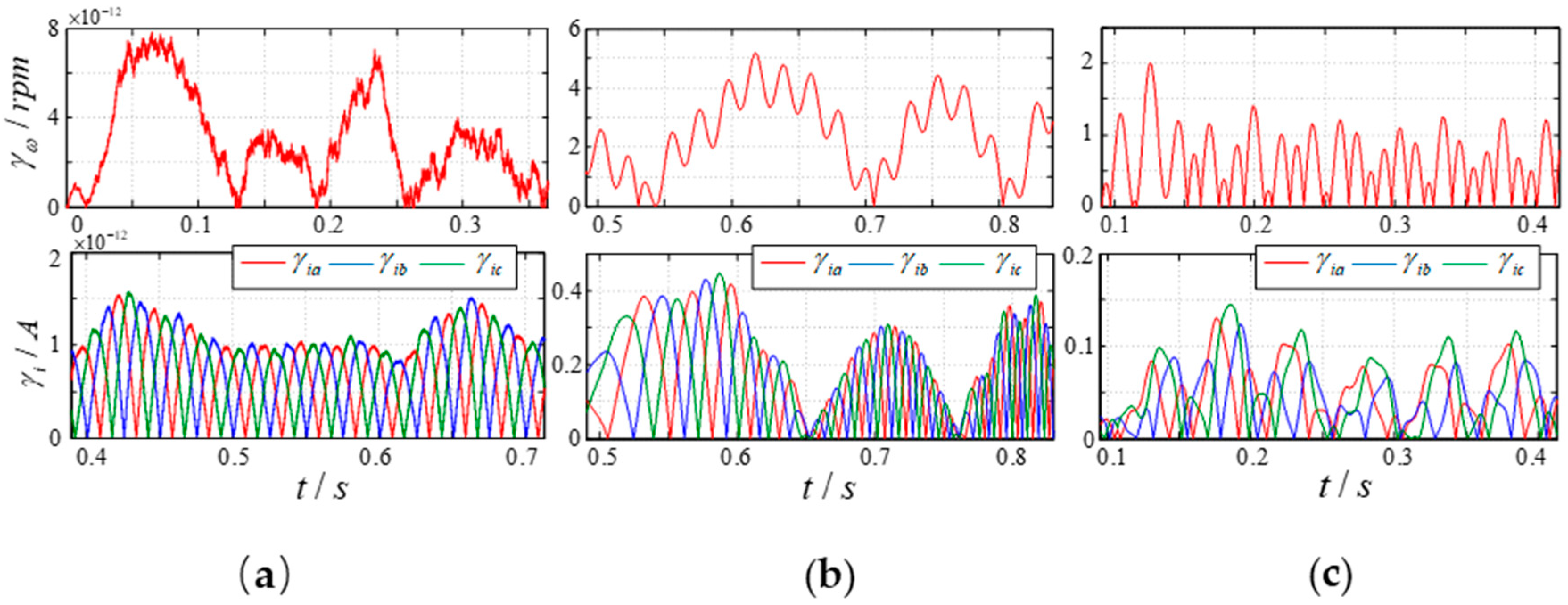
Before simulating the sensor fault diagnosis and fault-tolerant control, the thresholds of three-phase current and speed signals need to be set first. PMSM under no-load operation, under 40% demagnetization of the permanent magnet and under rated load is separately simulated, and corresponding simulation waveforms for the residuals of the current and speed signals are shown in Figure 3. Comparing the three simulation waveforms, the corresponding residuals of the signals under 40% demagnetization of the permanent magnet shown in Figure 3b are all higher than the other two cases, which is γ_iabcmax = 0.4 A, γ_ωmax ≈ 5 rpm.

Therefore, by searching for the maximum value of the residuals globally and leaving a certain margin, we can determine the fault thresholds of the signals are Γ_ia = Γ_ib = Γ_ic = 2 A, Γ_ω = 9 rpm. The threshold is equivalent to the value determined by the existing threshold setting method mentioned above.

So based on the fault thresholds, simulation analysis and verification can be performed on fault diagnosis and fault tolerance of various types of sensors.

5.1. Simulation I

The operating characteristics of the PMSM closed-loop control system based on the composite sliding mode observer are analyzed in the case of no sensor fault to verify the effectiveness of the proposed sliding mode observer.

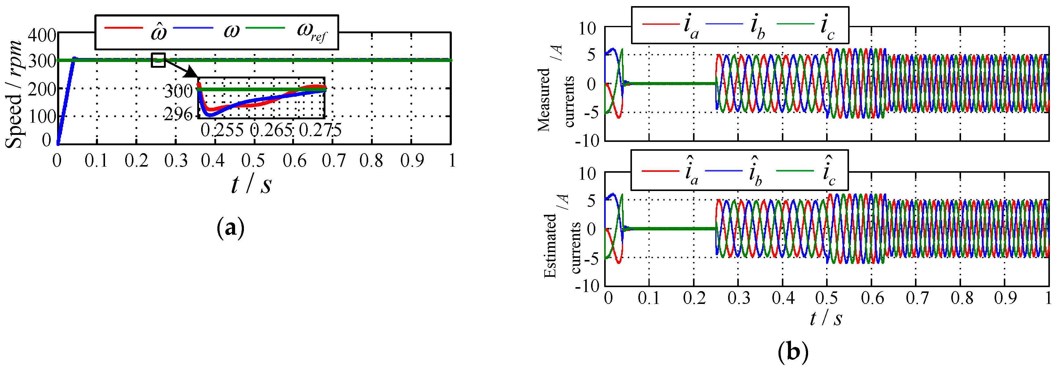
5.1.1. Normal Operation

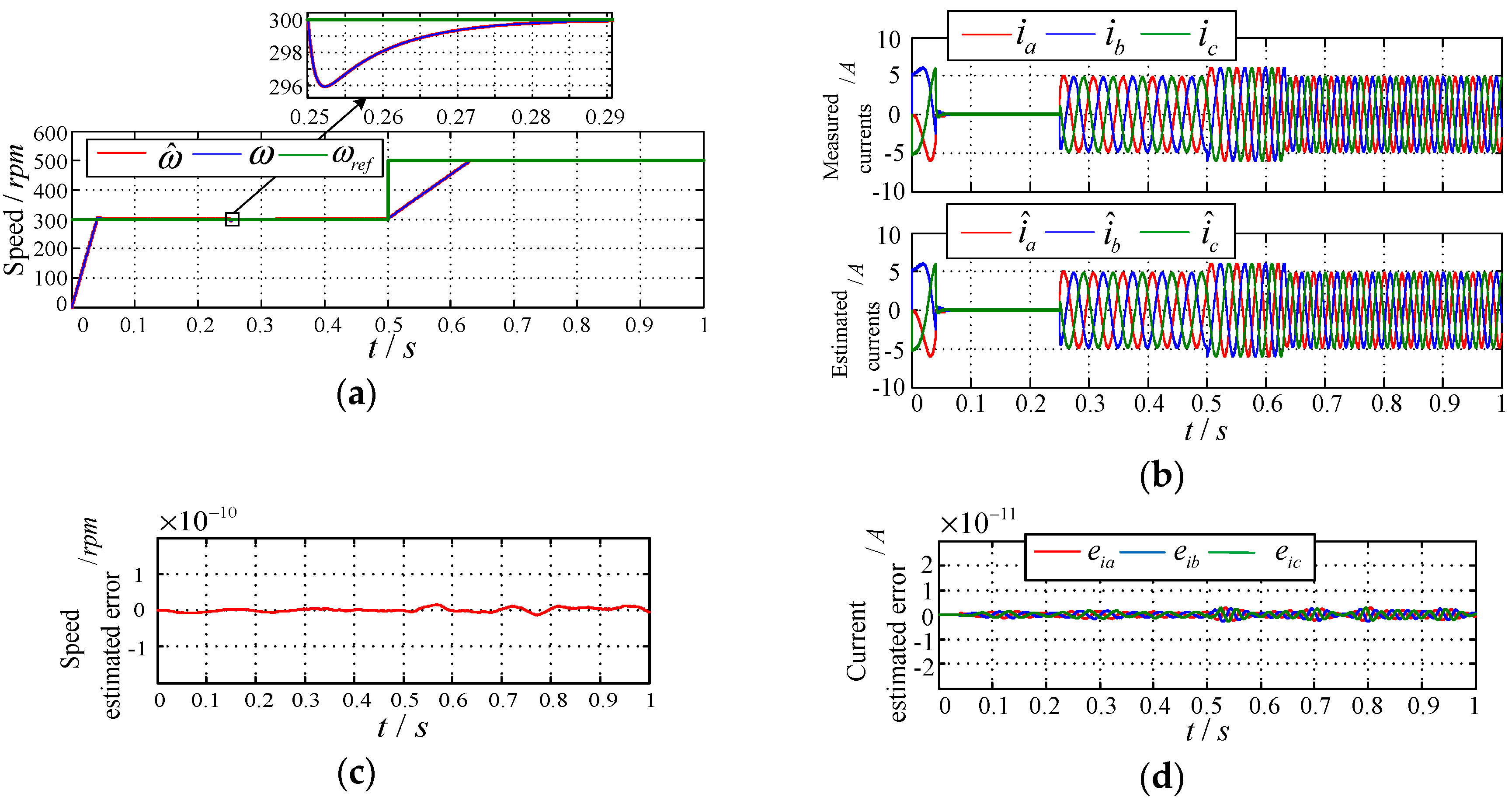
Assume the motor starts at t = 0 without load, and the given starting rotation speed is ω_ref = 300 rpm. After it is steady, apply a load torque T_L = 5 N·m at t = 0.25 s. At the moment t = 0.5 s, the given speed increases sharply to ω_ref = 500 rpm. The overall simulation time is 1 s, and the simulation result is shown in Figure 4.

It can be seen that the constructed composite sliding mode observer can estimate well the PMSM stator current and speed signals, and the error maintains at a small value near zero. When the system load torque or reference changes, the system fluctuations are small and the sliding mode tracking rate is fast. It indicates the good performance of the closed-loop control system and sliding mode control, thus verifying the effectiveness of the composite sliding mode observer proposed in this paper.

5.1.2. Disturbance Operation

Without loss of generality, the disturbance signal chosen in this paper is ξ(t) = 0.2sin(300t), and its distribution matrix Q = diag(1,1,−1) matches the matrix G_n. Similarly, the motor starts without load, with the given starting rotation speed being ω_ref = 300 rpm, and a disturbance signal ξ(t) is added to the system at the same time. After it is steady, apply a load torque T_L = 5 N·m at t = 0.25 s. The overall simulation time is 1 s, and the simulation result is shown in Figure 5.

Analysis of the waveforms shows that the interference signal added to the system does not affect the operation of the composite sliding mode observer and the estimated signal still matches the corresponding signal well. It is consistent with the previous theoretical analysis, and verifies the good robust performance and anti-disturbance performance of the composite sliding mode observer.

5.2. Simulation II

In this case, the effectiveness of the fault diagnosis and active fault-tolerant control strategy proposed in this paper is verified by simulating different types of sensor fault. In the simulation, it is assumed that there are three faults—a-phase current sensor being stuck, b-phase current sensor constant deviation, and speed sensor constant gain fault, and all faults occur at t_f = 0.6 s.

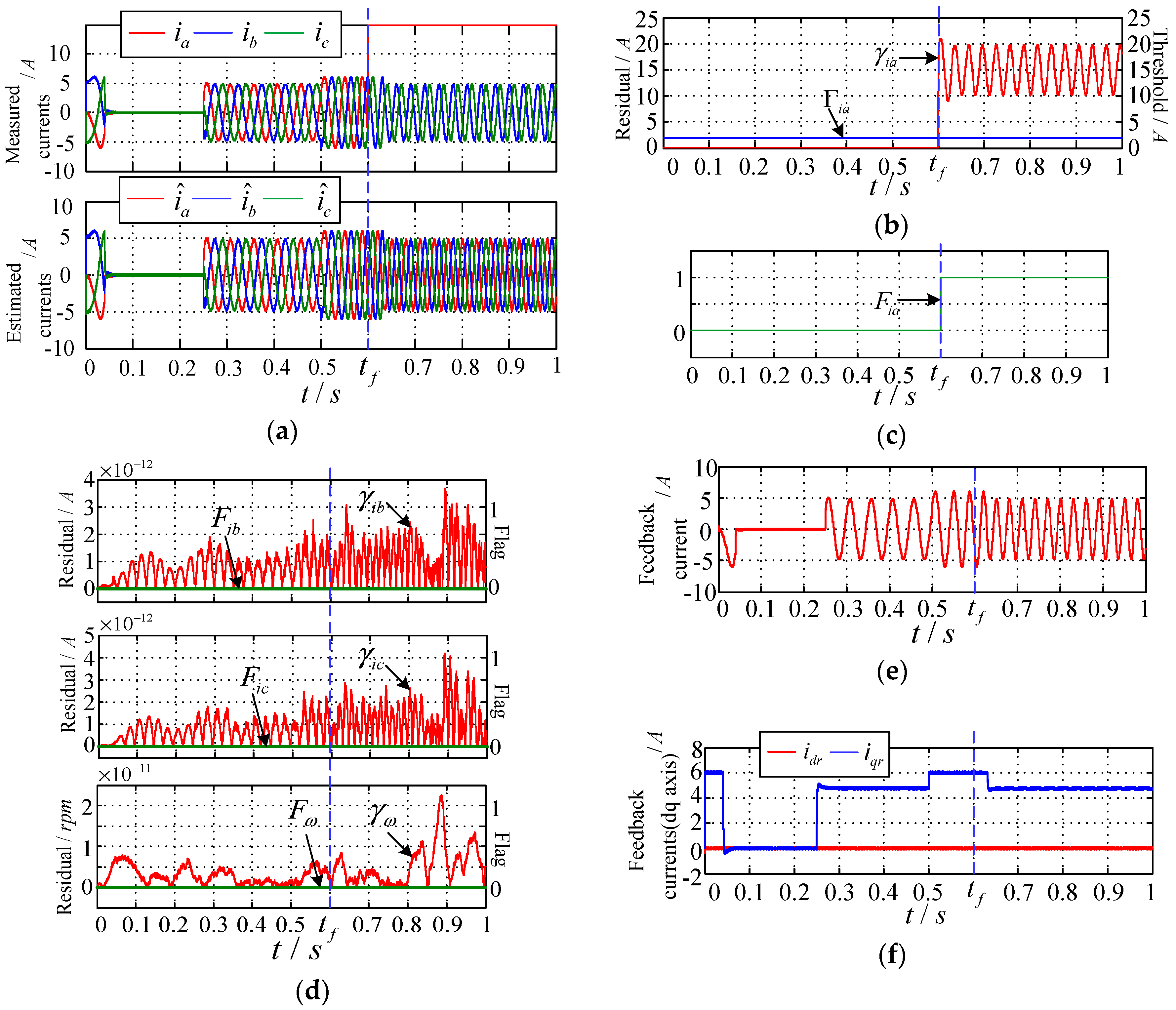
5.2.1. a-Phase Current Sensor Being Stuck

Assume K = 15 when the a-phase current sensor is stuck, and the corresponding simulation waveforms are shown in Figure 6.

It can be seen that at t = 0.6 s, the measured signal of a-phase stator current changes abruptly. At this time, the estimation of the three-phase stator current by the sliding mode observer is not affected, and the estimated current is still ${\widehat{i}}_a$, so ${\gamma }_{ia}=|i_a-{\widehat{i}}_a|>{\Gamma }_{ia}$. Then, F_ia changes from 0 to 1, indicating that the a-phase current sensor is faulty. However, the b-phase and c-phase current sensors and the speed sensor are working normally, and the residual is far less than the set threshold. The fault flag remains 0, which means that they are not affected by the $a$-phase current sensor failure. In this way, through fault-tolerant reconstruction and control of the feedback signal, the closed-loop feedback signals can be obtained, i_ar = 0 × i_a + 1 × ${\widehat{i}}_a$, i_br = i_b, i_cr = i_c, ω_r = ω. So the a-phase current feedback signal changes from the measured signal to the estimated signal at the time of failure, while the a-phase and a-phase current and speed feedback signals are still composed of the measured signals of corresponding sensors. Thus, the a-phase sensor fault does not produce adverse effects on the system. Further analysis of Figure 6f shows that the closed-loop feedback signal of three-phase current still maintains good symmetry, and the overall system control strategy and algorithm are not impacted by the a-phase current sensor fault, which ensures the safe and stable operation of the system.

5.2.2. b-Phase Current Sensor Constant Deviation

Assume n = 8 when the b-phase current sensor has a constant deviation fault, and the corresponding simulation waveforms are shown in Figure 7.

It can be seen that at t = 0.6 s, the measured signal i_b of b-phase stator current is superimposed a constant deviation. At this time, the estimation of the three-phase stator current by the sliding mode observer is not affected, and the estimated current is still ${\widehat{i}}_b$, so ${\gamma }_{ib}=|i_b-{\widehat{i}}_b|>{\Gamma }_{ib}$. Then, F_ib changes from 0 to 1, indicating that the b-phase current sensor is faulty. However, the a-phase and c-phase current sensors and the speed sensor are working normally, and the residual is far less than the set threshold. The fault flag remains 0, which means that they are not affected by the b-phase current sensor failure. In this way, through fault-tolerant reconstruction and control of the feedback signal, the closed-loop feedback signals can be obtained, i_br = 0 × i_b + 1 × ${\widehat{i}}_b$, i_ar = i_a, i_cr = i_c, ω_r = ω, so the b-phase current feedback signal changes from the measured signal to the estimated signal at the time of failure, while the a-phase and c-phase current and speed feedback signals are still composed of the measured signals of corresponding sensors. Thus, the b-phase sensor fault does not produce adverse effects on the system. Further analysis of Figure 7f shows that the closed-loop feedback signal of three-phase current still maintains good symmetry, and the overall system control strategy and algorithm are not impacted by the b-phase current sensor fault, which ensures the safe and stable operation of the system.

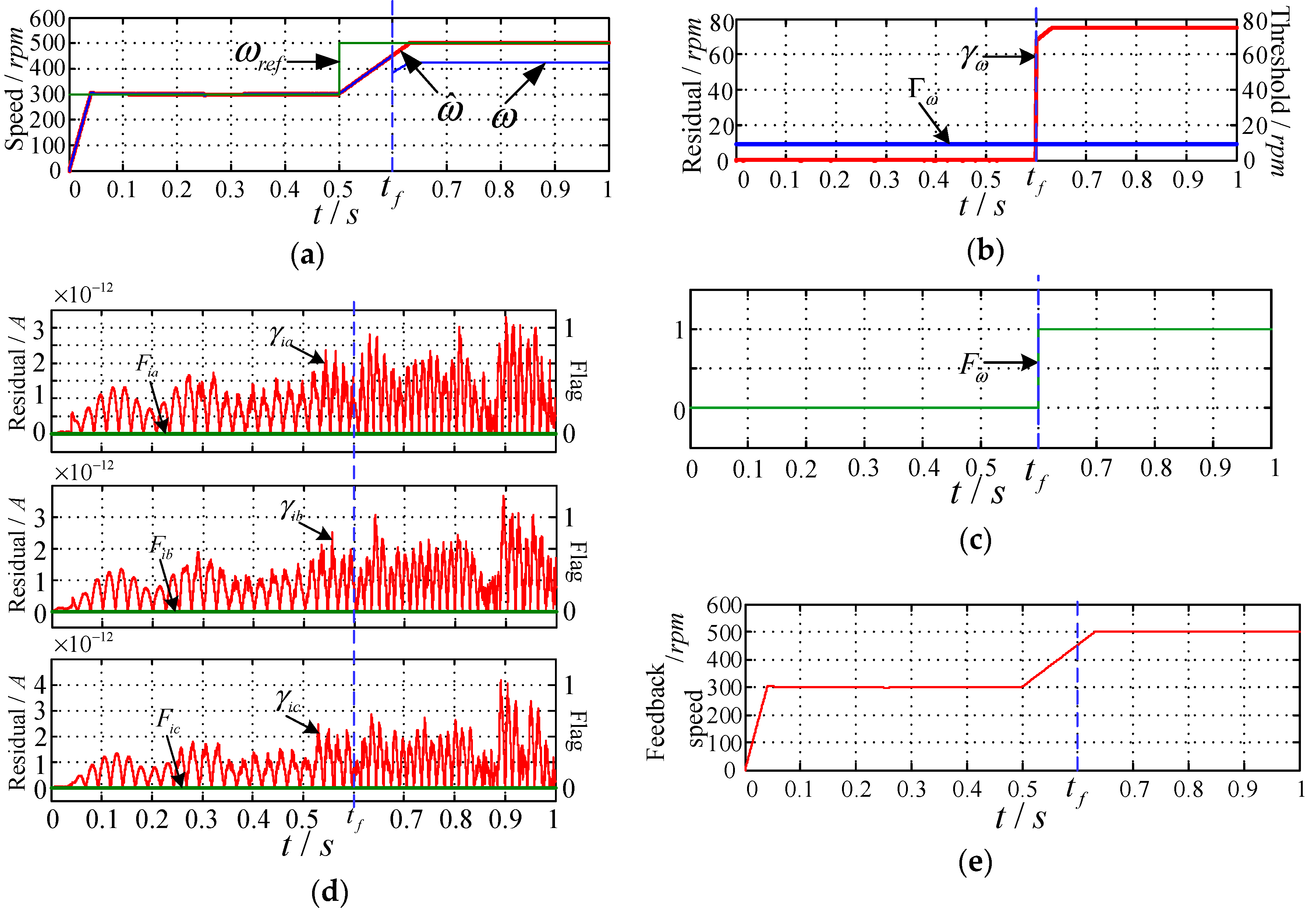
5.2.3. Speed Sensor Constant Gain Fault

Assume m = 0.85 when the speed sensor has a constant gain fault, and the corresponding simulation waveforms are shown in Figure 8. It can be seen that at t = 0.6 s, the measured signal of speed changes abruptly. At this time, the estimation of speed by the sliding mode observer is not affected, and the estimated speed is still $\widehat{\omega }$, so ${\gamma }_{\omega }=|\omega -\widehat{\omega }|>{\Gamma }_{\omega }$. Then, F_ω changes from 0 to 1, indicating the speed sensor is faulty. However, the three-phase current sensors are working normally, and the residual is far less than the set threshold. The fault flag remains 0, which means that it is not affected by the speed sensor failure. In this way, through fault-tolerant reconstruction and control of the feedback signal, the closed-loop feedback signals can be obtained, ω_r = 0 × ω + 1 × $\widehat{\omega }$ = $\widehat{\omega }$, i_ar = i_a, i_br = i_b, i_cr = i_c, so the speed feedback signal changes from the measured signal to the estimated signal at the time of failure, while the three-phase current feedback signals are still composed of the measured signals of corresponding sensors. Thus, the speed sensor fault does not produce adverse effects on the system.

Based on the simulation and analysis of the above three modes of failure, the effectiveness of the fault diagnosis and active fault-tolerant control strategy proposed in this paper is verified.

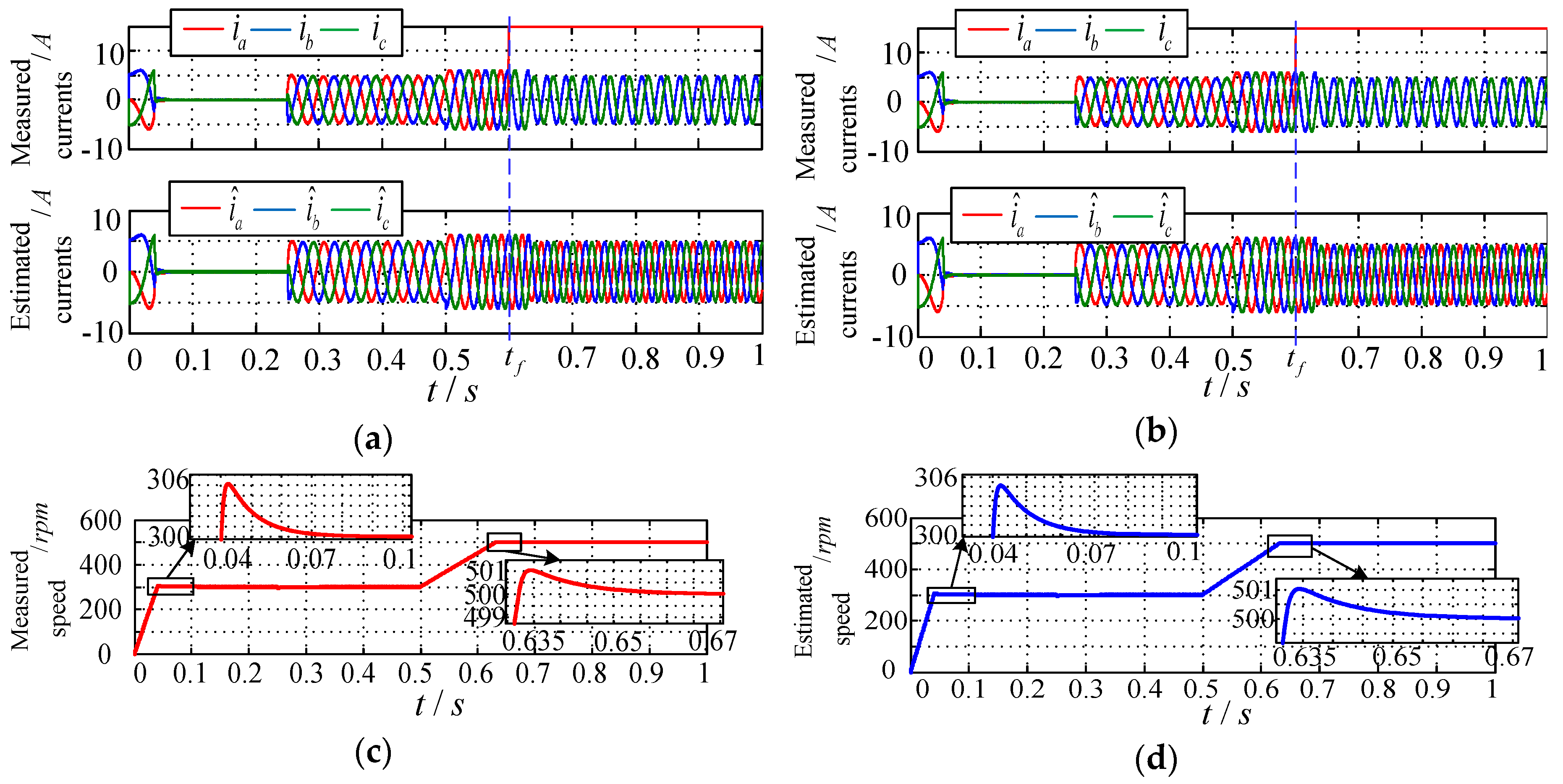
5.3. Simulation III

In this case, the design methods of the Luenberger observer oriented for motor speed sensor and current sensor and the traditional sliding mode observer in [10,12] are applied in the PMSM closed-loop control system constructed in this paper. The speed and three-phase current signals are observed and estimated to form a sensor fault diagnosis and fault-tolerant control system with multiple observers. Through simulation, its performance is compared with that of the proposed control system with a single composite sliding mode observer.

In the simulation, it is assumed that the a-phase current sensor is stuck (K = 15) and there is a speed sensor constant gain fault (m = 0.85), and the faults all occur at t_f = 0.6 s. The simulation output waveforms based on multi-observer and single composite observer system for different faults are shown in Figure 9, Figure 10 and Figure 11. The dynamic and steady-state performance indexes of the two types of system are calculated and shown in

Table 2. The dynamic and steady-state performance indexes based on different observers.

Type		Rise Time (s)		Adjust Time (s)		Steady-State Error (%)
		Speed	Current	Speed	Current	Speed	Current
Composite sliding mode observer		0.0361	0.0025	0.0995	0.0162	0.4	6.25
Multi-observer system	Traditional sliding mode observer	0.0362	-	0.0995	-	0.5	-
	Luenberger observer	-	0.0025	-	0.0165	-	6.3

.

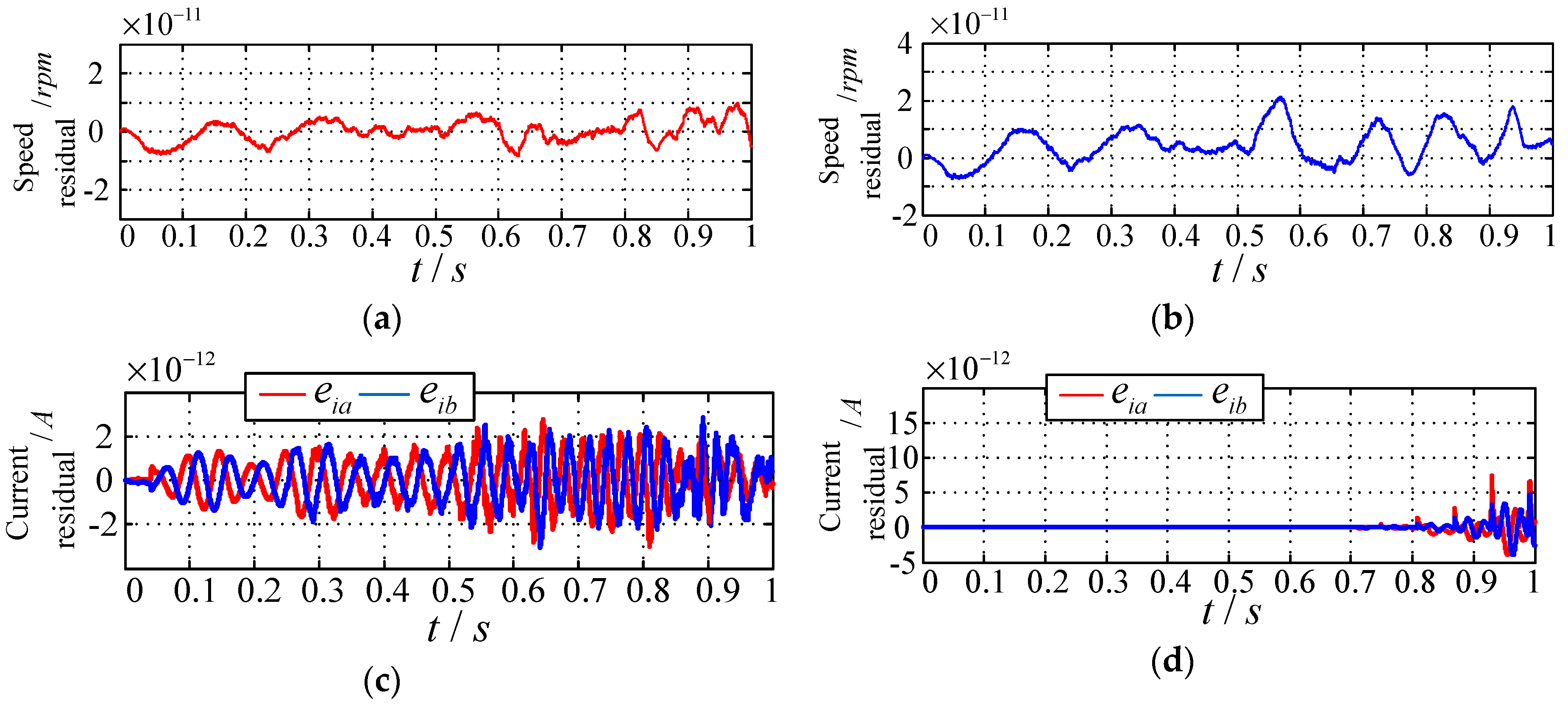
According to the above waveforms and data, it is not difficult to find that from the perspective of control objective, both the composite sliding mode observer control system proposed in this paper and the multi-observer control system based on [10,12] can realize diagnosis and fault-tolerant control under current and speed sensor faults, as shown in Figure 9a,b and Figure 10a,b. From the perspective of control accuracy, the composite sliding mode observer control system has higher precision and lower probability of misdiagnosis or missed diagnosis, and thus reducing the chattering phenomenon of the system considerably, as shown in Figure 9c,d, Figure 10c,d, Figure 11a and Figure 10d. From the perspective of control performance, the rise time and adjustment time of the composite sliding mode observer control system is shorter than that of the multi-observer control system, and the fault diagnosis and isolation control are more rapid, which can better meet the actual engineering application requirements. In addition, in the steady-state operation stage, the error between the steady-state response and the expected response is kept in a smaller range, which indicates its better steady-state performance, as shown in Table 2.

6. Conclusions

This paper, with the PMSM drive system as research object, studies the fault diagnosis and fault-tolerant control strategies after the failure of multiple sensors. The main work and contributions are as follows:

(1)

A composite sliding mode observer for multiple current and velocity signals in a PMSM drive system is proposed, which enables fast and accurate observation and estimation of different types of signals. It simplifies the implementation of observer-related algorithms and sensor fault diagnosis and isolation control algorithms, and facilitates engineering applications.

(2)

A method is proposed for determining fault thresholds by searching for the maximum impact of global steady-state error, parameter variation and load variation on residuals. The various factors of changing residuals are considered, which fully ensures the diagnostic accuracy of the system under different faults of different sensors.

(3)

The proposed fault diagnosis and fault-tolerant control strategy applies to three types of fault—stuck, constant gain and constant deviation of the three-phase current sensor and speed sensor of the PMSM drive system. Compared with the existing methods, the control strategy contributes to better dynamic, steady-state and anti-interference performance of the system, and can maintain stable operation of the system under severe working conditions. It can serve as reference for the reliability design of the motor drive system of electric vehicles.

The fault threshold of three-phase current and speed signals in this paper is based on the actual system simulation results and the application experience. There is still a lack of scientific theoretical basis, which is the problem that needs to be studied and solved in the future. Meanwhile, compared with the existing methods, the better dynamic, steady-state performance, and anti-disturbance performance of the proposed method in fault-tolerant control can be further verified by experiments.

References

1. Miyama, Y.; Hazeyama, M.; Hanioka, S.; Watanabe, N.; Daikoku, A.; Inoue, M. PWM Carrier Harmonic Iron Loss Reduction Technique of Permanent Magnet Motors for Electric Vehicles. IEEE Trans. Ind. Appl. 2016, 52, 2865–2871. [Google Scholar] [CrossRef]
2. Du, B.; Wu, S.; Han, S.; Cui, S. Interturn Fault Diagnosis Strategy for Interior Permanent-Magnet Synchronous Motor of Electric Vehicles Based on Digital Signal Processor. IEEE Trans. Ind. Electron. 2016, 63, 1694–1706. [Google Scholar] [CrossRef]
3. Zhongshi, Z.; Ruihai, M.; Lifang, W.; Junzhi, Z. Novel PMSM Control for Anti-Lock Braking Considering Transmission Properties of the Electric Vehicle. IEEE Trans. Veh. Technol. 2018, 67, 10378–10386. [Google Scholar]
4. Zhao, H.; Luo, P.; Wang, N.; Zheng, Z.J.; Wang, Y.T. Fuzzy Logic Control of the Fault-tolerant PMSM Servo System Based on MRAS Observer. In Proceedings of the 30th Chinese Control and Decision Conference (2018 CCDC), Shenyang, China, 9–11 June 2018; pp. 1812–1817. [Google Scholar]
5. Cai, B.P.; Zhao, Y.B.; Liu, H.L.; Xie, M. A Date-Driven Fault Diagnosis Methodology in Three-Phase Inverters for PMSM Drive Systems. IEEE Trans. Power Electron. 2017, 32, 5590–5600. [Google Scholar] [CrossRef]
6. Hao, Y.; Xu, Y.; Zou, J. A Phase Current Reconstruction Approach for Three-Phase Permanent-Magnet Synchronous Motor Drive. Energies 2016, 9, 853–868. [Google Scholar]
7. Khil, S.K.E.; Jlassi, I.; Estima, J.; Mrabet, B.; Cardoso, A.J.M. Current Sensor Fault Detection and Isolation Method for PMSM Drives, Using Average Normalized Currents. Electron. Lett. 2016, 52, 1434–1436. [Google Scholar] [CrossRef]
8. Wang, X.Q.; Wang, Z.; Xu, Z.X.; Cheng, M. Fault Diagnosis and Tolerance of Dual Three-phase PMSM Drives. In Proceedings of the 2018 IEEE Energy Conversion and Exposition (ECCE), Portland, OR, USA, 23–27 September 2018; pp. 325–330. [Google Scholar]
9. Grouz, F.; Sbita, L.; Boussak, M. Current Sensors Gain Faults Detection and Isolation based on an Adaptive Observer for PMSM Drives. In Proceedings of the 10th International Multi-Conference on Systems, Signals and Devices 2013 (SSD13), Hammamet, Tunisia, 18–21 March 2013; pp. 1–6. [Google Scholar]
10. Wu, C.; Guo, C.; Xie, Z.; Ni, F.; Hong, L. A Signal-Based Fault Detection and Tolerance Control Method of Current Sensor for PMSM Drive. IEEE Trans. Ind. Electron. 2018, 65, 9646–9657. [Google Scholar] [CrossRef]
11. Grouz, F.; Sbita, L.; Boussak, M. Current Sensors Faults Detection, Isolation and Control Reconfiguration for PMSM Drives. In Proceedings of the 2013 International Conference on Electrical Engineering and Software Applications, Hammamet, Tunisai, 21–23 March 2013; pp. 1–6. [Google Scholar]
12. Xia, J.; Guo, Y.; Dai, B.; Zhang, X. Sensor Fault Diagnosis and System Reconfiguration Approach for Electric Traction PWM Rectifier Based on Sliding Mode Observer. IEEE Trans. Ind. Appl. 2017, 53, 4768–4778. [Google Scholar] [CrossRef]
13. Veluvolu, K.C.; Kommuri, S.; Defoort, M.; Karimi, H.R. A Robust Observer-based Sensor Fault-Tolerant Control for PMSM in Electric Vehicles. IEEE Trans. Ind. Electron. 2016, 63, 7671–7681. [Google Scholar]
14. Kommuri, S.K.; Sang, B.L.; Veluvolu, K.C. Robust Sensors-Fault-Tolerance with Sliding Mode Estimation and Control for PMSM Drives. IEEE/ASME Trans. Mechatron. 2018, 23, 17–28. [Google Scholar] [CrossRef]
15. Foo, G.H.B.; Zhang, X.; Vilathgamuwa, D.M. Sensor Fault-Resilient Control of Interior Permanent-Magnet Synchronous Motor Drives. IEEE/ASME Trans. Mechatron. 2015, 20, 855–864. [Google Scholar]
16. Chybowski, L.; Twardochleb, M.; Wisnichi, B. Multi-criteria Decision Making in Components Importance Analysis Applied to a Complex Marine System. Nase More 2016, 63, 264–270. [Google Scholar] [CrossRef]
17. Zhang, G.Q.; Wang, G.X.; Wang, G.L.; Huo, J.Y.; Zhu, L.H.; Xu, D.G. Fault Diagnosis Method of Current Sensor for Permanent Magnet Synchronous Motor Drives. In Proceedings of the 2018 International Power Electronics Conference (IPEC-Niigata 2018-ECCE Asia), Niigata, Japan, 20–24 May 2018; pp. 1206–1211. [Google Scholar]
18. Tang, X.; Wang, X.H.; Li, Y.; Yang, Y.B.; Zhang, R. Demagnetization Study for Line-start Permanent Magnet Synchronous Motor During Starting Process. Proc. CSEE 2015, 35, 961–970. [Google Scholar]
19. Huangfu, Y.; Wang, S.; Rienzo, L.D.; Zhu, J. Radiated EMI Modeling and Performance Analysis for PWM PMSM Drive System Based on Field-circuit Coupled FEM. IEEE Trans. Magn. 2017, 53, 1–4. [Google Scholar] [CrossRef]
20. Corradini, M.L.; Ippoliti, G.; Longhi, S.; Orlando, G. A Quasi-Sliding Mode Approach for Robust Control and Speed Estimation of PM Synchronous Motors. IEEE Trans. Ind. Electron. 2012, 59, 1096–1104. [Google Scholar] [CrossRef]
21. Im, J.H.; Kim, R.Y. Improved Saliency-based Position Sensorless Control of Interior Permanent-magnet Synchronous Machines with Single DC-Link Current Sensor using Current Prediction Method. IEEE Trans. Ind. Electron. 2018, 65, 5335–5343. [Google Scholar] [CrossRef]
22. Abdelrahem, M.; Hackl, C.M.; Kennel, R. Finite Position Set-Phase Locked Loop for Sensorless Control of Direct-Driven Permanent-Magnet Synchronous Generators. IEEE Trans. Power Electron. 2018, 33, 3097–3105. [Google Scholar] [CrossRef]
23. Zhou, C.; Yang, G.; Su, J.; Sun, G. The Control Strategy for Dual Three-phase PMSM Based on Normal Decoupling Transformation under Fault Condition Due to Open Phases. Trans. China Electrotech. Soc. 2017, 32, 86–96. [Google Scholar]
24. Cunha, G.D.; Adalberto, J.R.; Alves, J.A.; Eduardo, C. Control of Permanent Magnet Synchronous Machines for Subsea Applications. IEEE Trans. Ind. Appl. 2017, 54, 1899–1905. [Google Scholar] [CrossRef]
25. Zhao, K.; Yin, T.; Zhang, C.; He, J.; Li, X.; Chen, Y.; Zhou, R.; Leng, A. Robust Model-free Nonsingular Terminal Sliding Mode Control for PMSM Demagnetization Fault. IEEE Access 2019, 7, 15737–15748. [Google Scholar] [CrossRef]
26. Sellami, T.; Berriri, H.; Jelassi, S.; Darcherif, M.A.; Mimouni, F.M. Short-Circuit Fault Tolerant Control of a Wind Turbine Driven Induction Generator Based on Sliding Mode Observers. Energies 2017, 10, 1611. [Google Scholar] [CrossRef]
27. Ma, Z.; Zhang, X. FPGA Implementation of Sensorless Sliding Mode Observer with a Novel Rotation Direction Detection for PMSM Drives. IEEE Access 2018, 6, 55528–55536. [Google Scholar] [CrossRef]
28. Xu, L.; Zhao, J.W.; Song, J.C.; Song, X.W.; Dong, F.; Zong, K.F. Research on Uniform Demagnetization Diagnosis of Permanent Magnet Synchronous Linear Motors Based on ALE-MRAS Flux Observers. Proc. CSEE 2019. Available online: http://kns.cnki.net/kcms/detail/11.2107.tm.20190227.1119.005.html (accessed on 22 April 2019).
Figure 1. The schematic diagram of fault diagnosis and active fault-tolerant control system based on sliding mode.
Energies 12 01695 g001
Figure 2. The block diagram of active fault-tolerant control.
Energies 12 01695 g002
Figure 3. The current and speed residual waveforms of the PMSM drive system. (a) No-load operation; (b) 40% demagnetization of the permanent magnet; (c) rated load
Energies 12 01695 g003
Figure 4. The simulation waveforms of PMSM drive system based on the composite sliding mode observer in the case of no sensor fault. (a) The given speed ωref, the measured speed ω, and estimated speed ω ^ ; (b) The measured signal iabc and estimated signal i ^ a b c of the three-phase stator current; (c) The estimated error of rotation speed eω; (d) The estimated error of current ei.
Energies 12 01695 g004
Figure 5. The simulation waveforms of PMSM drive system based on the composite sliding mode observer in the case of disturbance. (a) The given speed ωref, the measured speed ω, and estimated speed ω ^ ; (b) The measured signal iabc and estimated signal i ^ a b c of the three-phase stator current.
Energies 12 01695 g005
Figure 6. The system simulation waveforms when the a-phase current sensor is stuck. (a) The measured signal iabc and estimated signal i ^ a b c of the three-phase stator current; (b) a-phase current residual γia and threshold Γia; (c) The fault flag Fia of a-phase current sensor; (d) b-phase and c-phase current and speed residuals and fault flags; (e) a-phase closed-loop feedback current iar; (f) Closed-loop feedback current idqr in the dq coordinate system.
Energies 12 01695 g006
Figure 7. The system simulation waveforms in the case of constant deviation fault. (a) The measured signal iabc and estimated signal i ^ a b c of the three-phase stator current; (b) b-phase current residual γib and threshold Γib; (c) The fault flag Fib of b-phase current sensor; (d) a-phase and c-phase current and speed residuals and fault flags; (e) b-phase closed-loop feedback current ibr; (f) Closed-loop feedback current idqr in the dq coordinate system.
Energies 12 01695 g007
Figure 8. The system simulation waveforms in the case of speed sensor constant gain fault. (a) The given speed ωref, measured speed ω and estimated speed ω ^ ; (b) Speed residual γω and threshold Γib; (c) The fault flag Fω of speed sensor; (d) Three-phase current residuals and fault flags; (e) Closed-loop feedback speed ωr.
Energies 12 01695 g008
Figure 9. The observed signal output waveforms of two types of system when the a-phase current sensor is stuck. (a) The measured current iabc and estimated current i ^ a b c based on composite sliding mode observer; (b) The measured current iabc and estimated current i ^ a b c based on traditional sliding mode observer (Multi-observer system); (c) The estimated speed ω ^ based on composite sliding mode observer; (d) The estimated speed ω ^ based on Luenberger observer (multi-observer system).
Energies 12 01695 g009
Figure 10. The observed signal output waveforms of two types of system in the case of speed sensor constant gain fault. (a) The measured speed ω and estimated speed ω ^ based on composite sliding mode observer; (b) The measured speed ω and estimated speed ω ^ based on Luenberger observer (Multi-observer system); (c) The estimated current i ^ a b c based on composite sliding mode observer; (d) The estimated current i ^ a b c based on traditional sliding mode observer (multi-observer system).
Energies 12 01695 g010
Figure 11. The estimation error waveforms of observation signals of two types of system under normal operating conditions. (a) The speed estimation error based on composite sliding mode observer; (b) The speed estimation error based on Luenberger observer (multi-observer system); (c) The current estimation error based on composite sliding mode observer; (d) The current estimation error based on traditional sliding mode observer (multi-observer system).
Energies 12 01695 g011