Quantitative Inversion of Fixed Carbon Content in Coal Gangue by Thermal Infrared Spectral Data

Abstract

Fixed carbon content is an important factor in measuring the carbon content of gangue, which is important for monitoring the spontaneous combustion of gangue and reusing coal gangue resources. Although traditional measurement methods of fixed carbon content, such as chemical tests, can achieve high accuracy, meeting the actual needs of mines via these tests is difficult because the measurement process is time consuming and costly and requires professional input. In this paper, we obtained the thermal infrared spectrum of coal gangue and developed a new spectral index to achieve the automated quantification of fixed carbon content. Thermal infrared spectroscopy analyses of 42 gangue and three coal samples were performed using a Turbo FT thermal infrared spectrometer. Then, the ratio index (RI), difference index (DI) and normalized difference index (NDI) were defined based on the spectral characteristics. The correlation coefficient between the spectral index and the thermal infrared spectrum was calculated, and a regression model was established by selecting the optimal spectral DI. The model prediction results were verified by a ten times 5-fold cross-validation method. The results showed that the mean error of the proposed method is 5.00%, and the root mean square error is 6.70. For comparison, the fixed carbon content was further predicted by another four methods, according to the spectral depth H, spectral area A, the random forest and support vector machine algorithms. The predicted accuracy calculated by the proposed method was the best among the five methods. Therefore, this model can be applied to predict the fixed carbon content of coal gangue in coal mines and can help guide mine safety and environmental protection, and it presents the advantages of being economic, rapid and efficient.

1. Introduction

Gangue is the main solid waste in coal mine areas. In China, there are more than 1700 coal waste piles, totaling approximately 4.5 billion tons, with a rate of increase of 350 million tons per year [1]. The long-term accumulation of a large amount of gangue will have a serious impact on the ecological environment of the mining area [2,3]. For example, after rain, harmful substances in coal gangue infiltrate and pollute soil and groundwater in the mining area. After spontaneous combustion, coal gangue will produce harmful gases, such as carbon monoxide, which will pollute the atmospheric environment of the mining area. Improper handling of gangue may cause landslides, explosions and other accidents and poses a negative impact on the safety of mining areas [4,5].

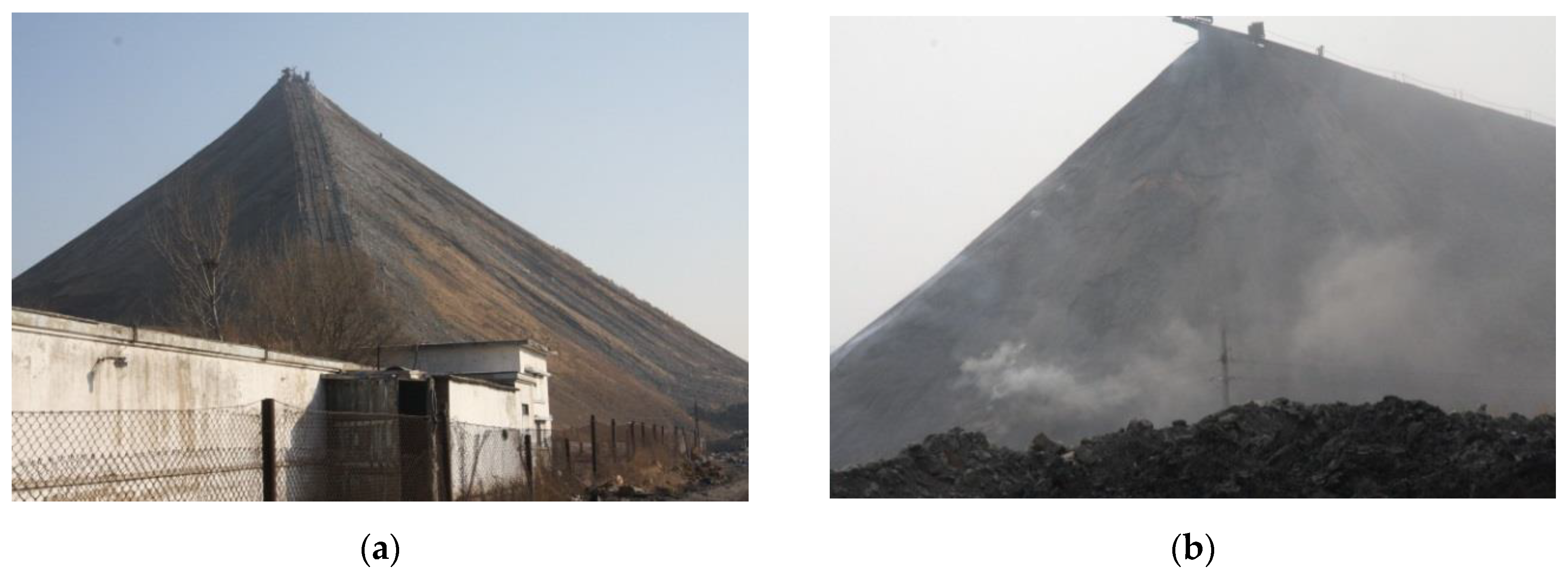
Carbonaceous gangue is an important part of coal gangue and has a low carbon content and certain calorific value and is flammable. Large coal gangue is located in the lower part of the coal gangue mountain, and small coal gangue is located in the upper middle part. Large gaps are observed within the large coal gangue in the lower part, and they allow for the passage of oxygen; and the small coal gangue in the middle and upper parts is weathered into granular gangue, which acts as a closed air system to prevent heat from being emitted. The spontaneous combustion of coal gangue continuously accumulates heat [6]. Gangue with a higher carbon content corresponds to higher heat released by combustion and a greater risk of spontaneous combustion.

At present, scholars in China and abroad mainly focus on the treatment and effective use of coal gangue. In the process of discharging gangue, if the fixed carbon content in the carbon-containing gangue can be monitored promptly and accurately and then classified according to the carbon content, the possibility of spontaneous combustion of coal gangue can be greatly reduced [7]. However, the comprehensive utilization of gangue with different carbon contents varies. For example, gangue with high carbon content can be used as fuel for generating electricity, and gangue with low carbon content is used to produce brick and other building materials [8,9,10]. Thus, it is very helpful to quickly and accurately determine the fixed carbon content in coal gangue to ensure that it is effectively utilized.

At present, the traditional method for precisely determining fixed carbon is measurement by chemical tests, although these tests are time consuming and costly, which reduces their efficiency in meeting the demands of the mine. Compared to the traditional proximate analysis method, some new methods, such as the thermogravimetric (TG) [11], the differential thermogravimetry (DTG) [12] and differential scanning calorimetry (DSC) [13] were developed to predict the fixed carbon content of the coal, the error between the predicted content and chemical test results was less than 1%. However, the real-time monitoring of fixed carbon content cannot be satisfied by these methods, although the predicted accuracy was relatively high.

With the development of the near-infrared spectroscopy technology, the rapid, non-contacting and nondestructive method for fixed carbon content monitoring can be realized and widely applied in a variety of samples, including coal [14], bamboo [15] and corn stover [16]. For the prediction of fixed carbon content in coal, Le et al. combined the near-infrared reflectance spectroscopy and the extreme learning machine algorithm to predict the fixed carbon content in coal, the root mean square error (RMSE) of predicted content and chemical test results was 3.2570% [17]; Kim et al. predicted the fixed carbon content on line based on the near-infrared spectroscopy is not different from that of traditional methods at 90% confidence level [18]; Xie et al. analyzed the biochar quantitatively and the results showed that the coefficient R of the predicted result is 0.9423, and the root mean square error is 0.1074 [19]. In addition, Yao et al. developed a rapid coal analyzer based on laser-induced breakdown spectroscopy (LIBS) and nonlinear regression method for coal samples, which can quickly and accurately predict fixed carbon content [20].

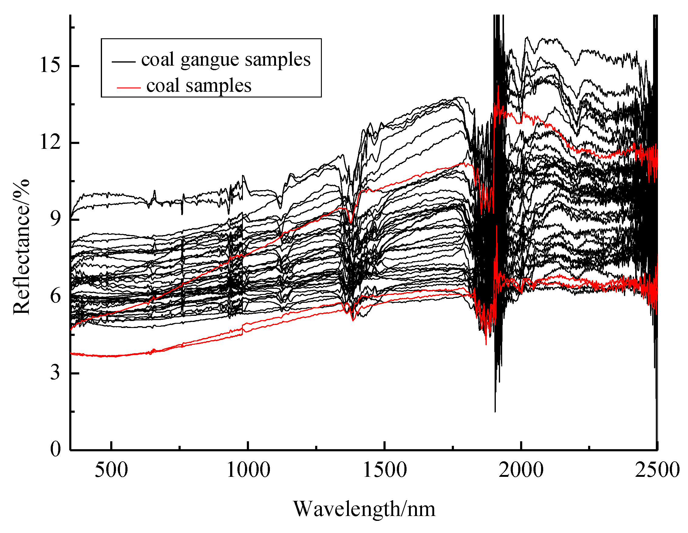
Some coal gangues are gray and black in color similar to coal. Additionally, the visible, near-infrared spectroscopy of the two can often be mixed and difficult to distinguish [21]. Therefore, it is difficult to accurately predict the fixed carbon content of coal gangue based on near-infrared spectroscopy.

In recent years, with the rapid development and wide application of thermal infrared spectroscopy, this method has frequently been used for the quantitative analysis of components in materials. A large number of studies on the thermal infrared spectrum of soil have been conducted to predict moisture [22], sand content [23], salt content [24], organic carbon [25] and phosphorus content [26]. Zhang et al. established regression models of thermal infrared spectra for the CaO and SiO₂ contents in rocks by using the field thermal infrared spectra of the rock samples, thus providing a new method of identifying rock types and mineral resources [27,28]. Feng et al. predicted the total sulfur content of cores and cut-rock surfaces based on the thermal infrared reflectance [29]. Another major application area of thermal infrared spectroscopy is the determination and content prediction of the surface components of the Moon and Mars [30,31,32,33,34].

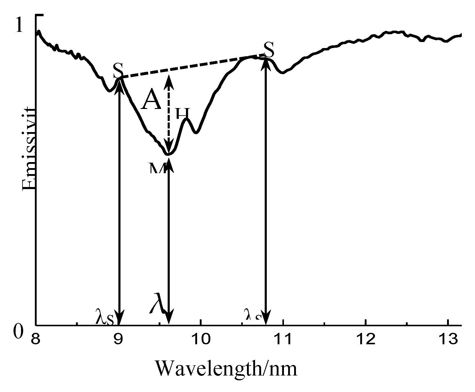
In this paper, the carbon-containing gangue samples in the Tiefa mining area are selected as the study object. First, the thermal infrared spectrum data of the samples were tested outdoors. Then, regression models on the thermal infrared spectrum and fixed carbon content were established. A new method of quantitatively inverting the fixed carbon content of carbonaceous gangue was proposed based on thermal infrared spectroscopy. The prediction results are compared with the results predicted by methods that use the spectral depth H, spectral absorption area A, random forest algorithm and support vector machine algorithm. The comparison results show that the proposed method has the best prediction effect. This new method has the advantages of being economic and efficient for determining carbon content in gangue.

2. Materials and Methods

2.1. Sample Collection

The Tiefa Coal Mine is located in Diaobingshan City (Liaoning Province, China, 42.4° N, 123.6° E). The coal mine has been in operation for more than 60 years, and its coal reserves are estimated at approximately 2 billion tons. This mine is an important coal production base in Liaoning Province. The coal in this mining area mainly consists of long flame coal and gas coal, which mostly have high ash and low sulfur contents. The coal is mainly used for power generation, boiler heating, etc.

Similarly, due to mining in the coal mining area, 16 coal gangue dumps were formed around the Tiefa mining area and had a great impact on the mining environment [35]. Since some coal gangue dumps are burning, it is necessary to quickly solve the environmental problems caused by the gangue dumps, as shown in Figure 1.

Forty-two samples of carbonaceous gangue (Nos. 1–42) were collected from different gangue dumps in the study area, and each sample had dimensions of approximately 8 cm × 8 cm × 4 cm. To ensure the accuracy of the inversion results, coal samples with higher fixed carbon content were used as the upper limit of gangue. In addition, three coal samples (Nos. 43–45) were collected in the coal yard, and industrial analysis of the coal samples was carried out according to national standard of China (GB/T214-2007, GB/T212-2008). The main industrial indices are shown in

Table 1. Test results for the proximate and ultimate analysis of coal samples.

Sample Number	Fixed Carbon/%	Moisture Content/%	Ash Content/%	Volatiles/%	Total Sulfur (Moisture Free)/%
43	36.64	3.18	32.21	27.97	0.46
44	42.32	5.30	23.83	28.55	0.42
45	44.72	6.69	18.42	30.17	0.46

.

2.2. Composition and Spectrum Acquisition of the Samples

2.2.1. Chemical Analyses

To reduce the experimental error and ensure the unity of the spectral tests and laboratory results, after each sample′s spectral observation was completed, the markers consistent with the size of the observation area were fixed on the sample surface, and the center of the marker coincided with the observation center. After all the experiments were completed, the upper surface of the sample area was cut down (or worn down) for chemical analysis. The fixed carbon content distribution of the sample is shown in Figure 2.

The gangue samples were numbered 1–42 according to the fixed carbon content from low to high, with the lowest content at 0.02% and the highest content at 31.22%. Table 1 shows that the fixed carbon content of the three coal samples (43–45) was above 36.64%. The highest carbon content of coal gangue was close to the carbon content of the coal samples. Figure 2 shows that the fixed carbon content of the Nos. 1–42 gangue samples was basically evenly distributed. This result indicates that the fixed carbon content of the collected coal gangue samples does not present a clustering effect and can thus effectively indicate the fixed carbon distribution of the waste in the coal mining area.

2.2.2. Visible, and Near-Infrared Spectrum

The samples were conducted in spectral test by using a SVC HR-1024 portable spectroradiometer (Spectra Vista Corporation, Poughkeepsie, NY, USA). The instrument measures in 1024 spectral bands, and it has three different resolutions in the 350–2500 nm spectral range, which are 5 nm in the 350–1000 nm region, 9.5 nm in the 1000–1850 nm region and 6.5 nm in the 1850–2500 nm region.

In order to minimize the impact of environmental factors, the experiment chooses sunny and cloudless weather. The spectral test time is between 10:00 to 14:00. The solar elevation angle is greater than about 45°. For the experiment, a 4° lens was used, and the minimum integration time of the sample was set to 3 ms. Each sample was tested three times and the average was taken as the final result. The visible, near-infrared spectra of 42 coal gangues and three coal samples are shown in Figure 3. The spectral curve of coal gangue is black and the spectral curve of coal is red.

Figure 3 shows that the visible, near-infrared spectral characteristics of coal and coal gangue samples are substantially similar:

(1)

The reflectance of both the coal and coal gangue increase linearly with a gentle slope in the range of 350–2150 nm, and then decreases in the range of 2150–2500 nm;

(2)

There are two local valleys at 1400 and 1900 nm on the reflectance curves of both the coal and coal gangue, which are affected by the absorption of water vapor and hydroxyl in the atmosphere;

(3)

The variation amplitude of reflectance spectrum over the entire wave range is less than 10%.

The difference in visible, near-infrared spectral characteristics of the two is that there is a valley at 2200 nm on the curves of coal gangue, which is caused by the vibration of Al-O bonds. while, the valley on the curves of coal are not obvious. The fixed carbon content of coal samples is higher than that of coal gangue, but the results showed that the visible, near-infrared spectra of the gangue and coal samples present obvious “different objects with the same spectrum” phenomena [36]. Therefore, it is difficult to establish its relationship of the fixed carbon content based on the visible, near-infrared spectroscopy.

2.2.3. Theoretical Analysis of Thermal Infrared Spectrum

Visible, near-infrared spectroscopy and thermal infrared spectroscopy have different recognition effects on different minerals, and there is complementarity between the two. In this paper, the difference between coal and gangue in the visible, near-infrared spectra is not obvious; therefore, we try to solve this problem by performing a test on the thermal infrared spectrum.

In the outdoor condition, when the target is close to the Fourier transform infrared (FT-IR) spectrometer, the atmospheric effects can be minimized, and the spectral radiance reaching the spectrometer sensor, L₀(λ) can be defined by the following equation [37]:

$$L_0(\lambda )=\epsilon (\lambda )L_{\mathrm{bb}}(T_S,\lambda )+[1-\epsilon (\lambda )]L_{dwr}(\lambda ).$$

(1)

where T_s is the temperature of the sample surface (K); λ is the wavelength (μm); ε(λ) is the spectral emissivity of the sample surface; L_dwr(λ) is the downwelling radiance field in the experimental condition (W·m⁻²·μm⁻¹·sr⁻¹). L_bb(T_s,λ) is the spectral blackbody radiance at a target surface temperature of T_s (W·m⁻²·μm⁻¹·sr⁻¹). The static radiance of the sample is mainly related to three factors: the sample surface temperature, T_s; the surface emissivity, ε(λ); and the downwelling radiance, L_dwr(λ). Therefore, the emissivity can be calculated by the following Equation (2):

$$\epsilon (\lambda )=\frac{L_0(\lambda )-L_{\mathrm{dwr}}(\lambda )}{L_{bb}(T_S,\lambda )-L_{\mathrm{dwr}}(\lambda )}.$$

(2)

The sample radiance can be obtained by the FT-IR directly in the outdoor condition. And the sample temperature can be measured by the temperature tester. The L_bb(T_s,λ) can be calculated by the known temperature according to the plank’s law. Then, the L_dwr(λ) can be measured by the standard diffuse reflecting gold plate, with a known reflectivity of 0.97, placed in the same orientation and position as the target. The temperature of the gold plate was measured by the temperature tester as the input, and the L_dwr(λ) can be calculated [38].

2.2.4. Experimental Method of Thermal Infrared Spectrum

The thermal infrared spectra of 45 samples were obtained by the Turbo FT spectral radiometer designed by the Design & Prototypes Corporation (Simsbury, CT, USA). The spectral measurement range was 3–15 μm, the spectral resolution was 4 cm⁻¹, and the observation view angle was 4.8°. The observed distance was 30 cm, and the diameter was approximately 2.5 cm. Each sample was repeated 3 times, and the average emissivity was taken as the final observed value.

First, a liquid nitrogen-cooled spectrometer detector is required to ensure that the internal temperature remains constant for no less than 60 min. Then, cold-warm blackbody calibration is performed to reduce the influence of instrument noise on the experimental results. The irradiance of the sample can only be tested after calibration. Considering that the downwelling radiance was relatively strong in case of low clouds or heavy dust, the experiment was carried out with a cloudless, low-temperature, outdoor background in the evening. In addition, the background radiation was obtained by the diffuse gold plate every 10 min during the spectral test. The temperatures of both the sample and the gold plate were measured by a TWC-2A multichannel temperature meter (Guangzhou, China) including Pt1000 temperature probes. The measurement precision was ±0.3% rdg +1 °C in the range of 0 °C to 100 °C, and the resolution was 0.01 °C.

The results are shown in Figure 4. Taking the influence of the atmospheric window and observation environment on sample emissivity into account, the spectral data of 8–13 μm were selected for analysis.

The thermal infrared spectra of the coal samples (dotted line) showed that the value of emissivity of coal is above 0.95 in the band range of 8–13 μm and presents small fluctuations, and it is close to the black-body spectrum curve. The solid line represents the thermal infrared spectrum curve of the gangue sample, and its spectral characteristics are as follows:

(1)

In the 8.0–9.6 μm range, a declining trend is observed on the emissivity curve, and at a bandwidth between 8.0 and 8.5 μm the speed slows down. Then, a sharp decrease is observed after 8.5 μm, and then the emissivity value rapidly increases after a trough at 8.7 μm. A local wave peak was observed at 9.0 μm. The emissivity value reaches its minimum at 9.6 μm.

(2)

In the 9.6–10.8 μm range, the spectral curve basically increases, and a local peak occurs at 9.83 μm and a trough occurs near 10 μm.

(3)

In the 10.8–13.0 μm range, the emissivity spectrum slowly increases, and the change is small. There is a weak emission valley near 11.3 μm.

Figure 4 shows that the emissivity spectra of the coal and gangue samples are obviously different:

(1)

The spectral emissivity of coal is obviously higher than that of gangue, with the emissivity of coal above 0.95 and that of gangue from 0.75–0.95.

(2)

There is a strong emission valley in the 9–10.8 μm range of the gangue curve, and the coal samples have no characteristics in this band. In addition, there is a positive correlation between the carbon content of gangue and the depth of the trough, which indicates that a lower carbon content corresponds to a deeper trough.

2.3. Spectral Index Based on Sensitive Bands

According to the proposed normalized difference vegetation index (NDVI), similar spectral indices were developed, such as the normalized difference water index (NDWI) [39] and normalized difference building index (NDBI) [40]. These indices provide an effective methods of classifying and detecting target objects of remote sensing images. Many researchers have identified interesting features based on new spectral indices. For example, the spectral index was used to estimate the soil organic matter content [41], building area [42] and crop health [43].

Studies have shown that thermal infrared spectroscopy can effectively predict the organic carbon content in aerosols [44]. In this paper, we test the thermal infrared curve of gangue, and the results show that samples with different fixed carbon contents have different thermal infrared spectra. To further study the relationship between spectral characteristics and fixed carbon content and reduce the influence of the experimental environment on spectral characteristics, the difference index (DI), ratio index (RI) and normalized difference index (NDI) are constructed:

$$DI=R_{\lambda m}-R_{\lambda n}$$

(3)

$$RI=\frac{R_{\lambda m}}{R_{\lambda n}}$$

(4)

$$NDI=\frac{R_{\lambda m}-R_{\lambda n}}{R_{\lambda m}+R_{\lambda n}}$$

(5)

where R_λm and R_λn are the reflectance of random wavelengths from 350–2500 nm.

MATLAB (MathWorks, Natick, MA, USA) was used to calculate the correlation coefficients of the three spectral indices of the fixed carbon content and any two bands of DI, RI and NDI, and the absolute values of the correlation coefficients were calculated by the three spectral indices. The results are shown in Figure 5a–c. The maximum value of the correlation coefficient was selected, and the corresponding bands were sensitive bands for fixed carbon content and spectral index.

The horizontal and vertical coordinates in the figures above represent the wavelengths of the sample spectrum, and the different color fields correspond to the distribution of the absolute values of the correlation coefficients between the spectral indices (DI, RI and NDI) of the wavelengths and the fixed carbon content. The colors from blue to red indicate that the absolute value of the correlation coefficient of the two is gradually increased from 0 to 1. A deeper red color indicates a stronger correlation. The maximum of the correlation coefficient is found from the diagram, and the locations of the sensitive bands of the experimental sample are listed in

Table 2. Sensitive bands and correlation coefficients corresponding to different spectral indices.

Spectral Index	Sensitive Band/μm	Absolute Value of Correlation Coefficient
DI	9.853/10.024	0.8668
RI	9.853/10.024	0.8630
NDI	9.853/10.024	0.8626

DI: Difference index; RI: ratio index; NDI: Normalized difference index.

.

3. Results

3.1. Model Establishment and Verification

Table 2 shows that the selected sensitive bands of the spectral indices (DI, RI, and NDI) are located at 9.853 and 10.024 μm, and the sensitive band diagram is shown in Figure 4 (blue line). The correlation between the three spectral indices and the sensitive band is high and relatively close, whereas the correlation coefficient between DI and the fixed carbon content is the highest, at −0.8668, R² = 0.75. Therefore, the model is built according to the DI:

$$DI=R_{10.024}-R_{9.853}$$

(6)

$$C=-1684.943\times DI+25.161$$

(7)

where C is the fixed carbon content of the samples, and R_10.024 and R_9.853 represent the emissivity at 10.024 μm and 9.853 μm, respectively. The fitting result of the linear model is shown in Figure 6.

Figure 6 shows that the fixed carbon content of the sample is linearly related to the spectral index DI. After linear fitting, the fixed carbon content can be predicted based on DI. To further verify the correctness of the model, 15 samples were taken for the spectral test, and the thermal infrared spectra are shown in Figure 7.

Similarly, the fixed carbon content was tested, and the fixed carbon content in the samples was predicted by the above model. The results are shown in

Table 3. Test values and predicted values of fixed carbon for the validation samples.

Sample Number	Test Results	Predicted Value	Sample Number	Test Results	Predicted Value
46	1.44	12.16	54	16.37	14.14
47	2.76	4.75	55	16.99	10.47
48	2.77	12.21	56	17.72	17.09
49	3.9	17.73	57	21.18	13.44
50	4.02	9.66	58	24.72	25.47
51	5.69	18.35	59	25.51	19.10
52	6.02	13.32	60	32.05	20.15
53	13.96	16.31

.

To better verify the model proposed in this paper, the ten times 5-fold cross-validation method was used to test the classification accuracy of random forest [45]. That is, all samples were randomly divided into five subsamples, with four subsamples used as training samples and the remaining subsample used as the test samples. After five cycles, all samples were predicted only once, and the mean values of the classification results were evaluated as the 5-fold classification accuracy. To determine the accuracy of the classification, the above process was repeated ten times, and the average classification accuracy of these ten repetitions was used as the final classification result. The prediction results are shown in

Table 4. Prediction results of the proposed model.

Test Order	Average Error/%	RMSE	Test Order	Average Error/%	RMSE
1	4.97	6.72	6	4.98	6.78
2	4.98	6.65	7	5.04	6.71
3	5.00	6.71	8	4.97	6.67
4	5.01	6.67	9	5.00	6.69
5	5.02	6.69	10	5.02	6.69

RMSE: Root mean square error.

.

Table 4 shows the results of the ten times 5-fold cross validation and indicates that the proposed model has an average error of 5.00% and a root mean square error (RMSE) of 6.70.

3.2. Comparison of Different Methods

The above studies show that the proposed method can accurately predict the fixed carbon content in coal gangue. To further determine the advantages and disadvantages of the method, the experimental results are compared with the prediction results of other methods. The comparison mainly includes methods based on spectral absorption characteristics and support vector machine (SVM) and random forest (RF) algorithms. Both of these machine learning algorithms are widely used in remote sensing.

The RF algorithm is currently one of the most popular classification algorithms for data mining [46,47]. This algorithm is an integrated learning algorithm proposed by Breiman in 2001. The essence of this algorithm is to improve the decision tree algorithm. SVM is a machine learning algorithm proposed by Vipnik et al. based on statistical learning theory [48]. The main idea of the algorithm is to establish a classification hyperplane as a decision surface, which maximizes the isolation edge between positive and negative cases [49].

(1) Modeling method based on spectral absorption characteristics

The spectral absorption characteristic parameters are the main indices for describing the spectral characteristics of samples, including the spectral absorption depth (W), absorption width (d), absorption position (H) and spectral absorption area (A), which are defined as:

$$\mathrm{Absorption} \mathrm{width}: W=\lambda s_2-\lambda s_1$$

(8)

$$\mathrm{Absorption} \mathrm{symmetry}: d=\frac{\lambda s_2-\lambda m}{\lambda s_2-\lambda s_1}$$

(9)

Figure 7 shows the thermal infrared spectra of one typical coal gangue sample, which shows an absorption valley characteristic at 8–11 μm. In Figure 8, M is the absorption valley position and S₁ and S₂ are the absorption peak positions.

The spectra of the gangue sample show that samples of different carbon contents have different spectral depths (H) and areas (A). Moreover, the higher the fixed carbon content is of the sample, the lower the spectral depth and the smaller the spectral area. Therefore, we try to establish the relationship between the fixed carbon content and the spectral depth H and the spectral area A.

Based on the spectral absorption depth (H), 42 samples are modeled by the carbon content (C). The correlation coefficient is −0.526, and the fitting equation is as follows:

$$C=-190.077\times H+29.267$$

(10)

Based on the spectral absorption area (A), 42 samples are modeled by the carbon content (C). The correlation coefficient is −0.564, and the fitting equation is as follows:

$$C=-259.361\times A+29.976$$

(11)

The prediction results of the modeling samples and test samples are shown in

Table 5. Prediction results of absorption depth (H) and absorption area (A).

Results	Average Error of Modeling Sample/%	Average Error of Test Sample/%	RMSE of Modeling Sample	RMSE of Test Sample
absorption depth (H)	7.08	8.54	8.84	10.46
absorption area (A)	6.73	8.49	8.59	10.59

. The average error and RMSE are used for the accuracy evaluation of the results.

(2) Random Forest (RF)

The RF algorithm is widely used in various regression predictions. For example, the algorithm is used to predict the organic carbon content in soil [50], estimate the biomass of wetland vegetation [51], and estimate the PM2.5 concentration in the atmosphere [52].

All data are divided into a training set and a test set. The RF algorithm constructs the predictive model by learning the training set and then predicting the test set. In this paper, the fixed carbon content in gangue was regression predicted by using the spectral data of full bands as the independent variable. During the learning process, the number of trees N was set as 100. The RF algorithm also used a ten times 5-fold cross-validation method to evaluate the classification accuracy. RF algorithms were implemented by MATLAB R2009 (a).

(3) Support Vector Machine (SVM)

The SVM method is simple and robust and suitable for high-dimensional small sample prediction. This method has been applied in many fields, such as disease prediction and industrial fields [53,54]. In this paper, the SVM algorithm prediction is performed using the LIBSVM toolbox developed by Professor Lin Chih-Jen of Taiwan University via MATLAB. Similar to the RF algorithm, the input data of the SVM algorithm is a full-band spectrum. Cross validation is used to select the best parameters c and g during the SVM process. The SVM algorithm also used a ten times 5-fold cross-validation method to evaluate classification accuracy. The prediction results of the RF and SVM algorithms are shown in

Table 6. Prediction results of random forest and support vector machine algorithms.

Test Order	Average Error of Random Forest	RMSE of Random Forest	Average Error of SVM	RMSE of SVM
1	5.80	7.23	5.48	7.01
2	6.05	7.68	5.13	7.12
3	5.58	7.09	5.76	7.50
4	5.69	7.06	5.30	6.93
5	5.86	7.41	4.98	6.47
6	6.11	7.66	4.96	6.66
7	5.84	7.39	4.90	6.57
8	5.90	7.64	5.31	7.11
9	6.00	7.41	5.48	7.01
10	6.05	7.51	5.19	6.75

SVM: Support vector machine.

.

Then, the prediction results of the modeling method based on the sensitive band, absorption depth (H), absorption area (A), RF algorithm and SVM algorithm were analyzed, and the results are shown in

Table 7. Comparison of the prediction results of all samples for 5 different modeling methods.

Prediction Results	Average Error/%	Root Mean Square Error
sensitive band model	5.00	6.70
absorption depth (H)	7.47	9.29
absorption area (A)	7.20	9.16
random forest algorithm	5.89	7.41
support vector machine algorithm	5.25	6.92

.

Table 7 shows that among the five different modeling methods, the average error and the RMSE of the sensitive band model are 5.00% and 6.70, respectively. This model is superior to the other 4 methods because the prediction accuracy of the model is higher; thus, the model can be applied to the prediction of fixed carbon content of gangue.

4. Discussion

4.1. Mechanism Analysis

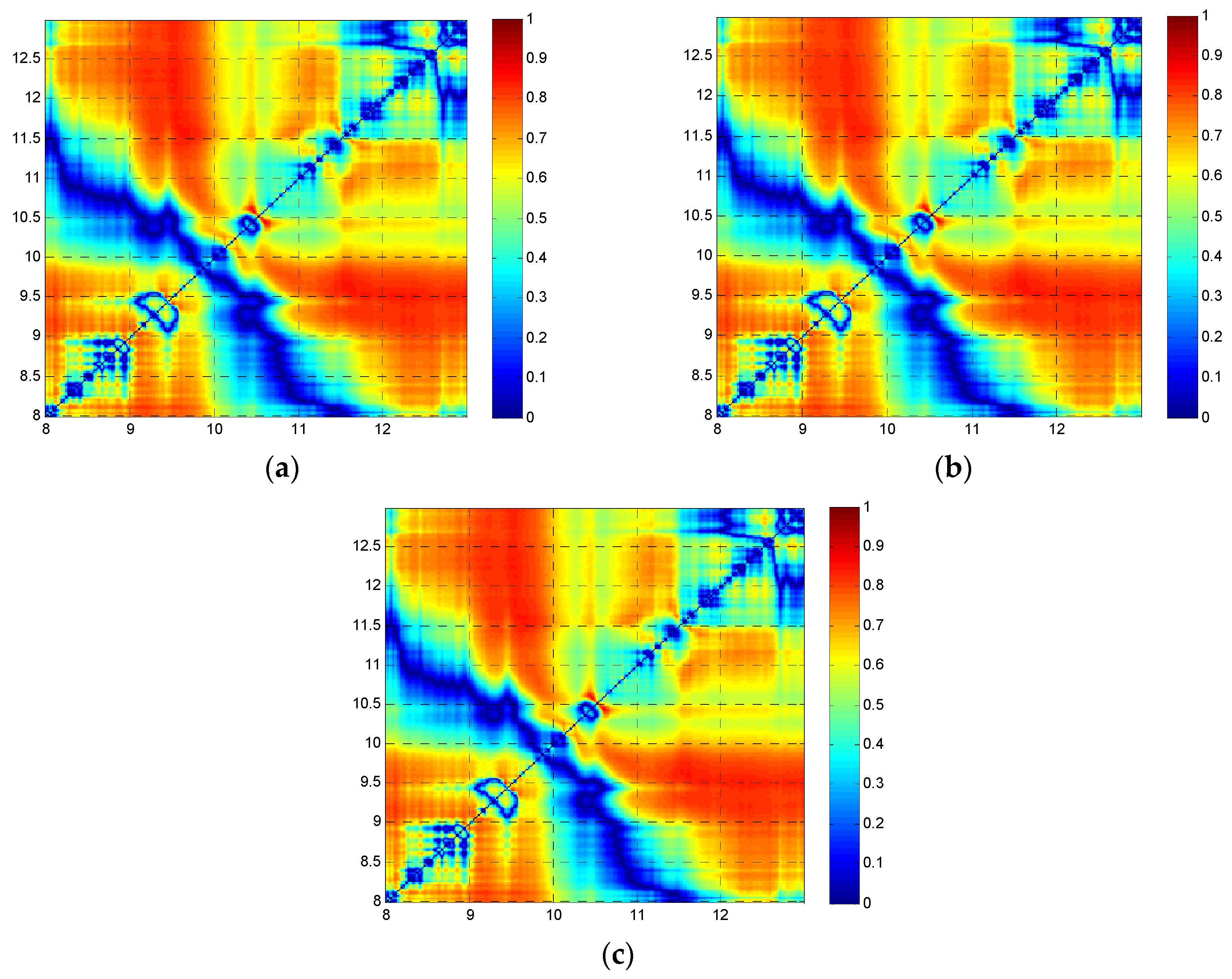
There is a linear relationship between the thermal infrared emissivity and the component content of the mixture. The spectrum of rock is composed of a linear mixture of mineral spectra of each component, and the proportion of the mineral spectra of each component in the mixed spectrum is the proportion of the mineral area to the rock surface area [55].

The carboniferous gangue in the Tiefa mining area mainly comes from thin coal seams and carbonaceous shale in the tunneling strata. To further understand its mineral composition, five sliced gangue samples were selected and observed under a polarizing microscope. The results show that the main minerals in the gangue are carbonaceous minerals and clay minerals (kaolinite) and a small amount of quartz, potassium feldspar, albite, muscovite and biotite. The carbonaceous minerals are opaque, fine and scattered and concentrated in banded or lump-like distributions. These minerals are black and brown, which makes the whole sample appear black, thus leading to similar reflectance spectra between coal and gangue in the visible, near-infrared bands, which results in the phenomenon of “different objects with a similar spectrum”.

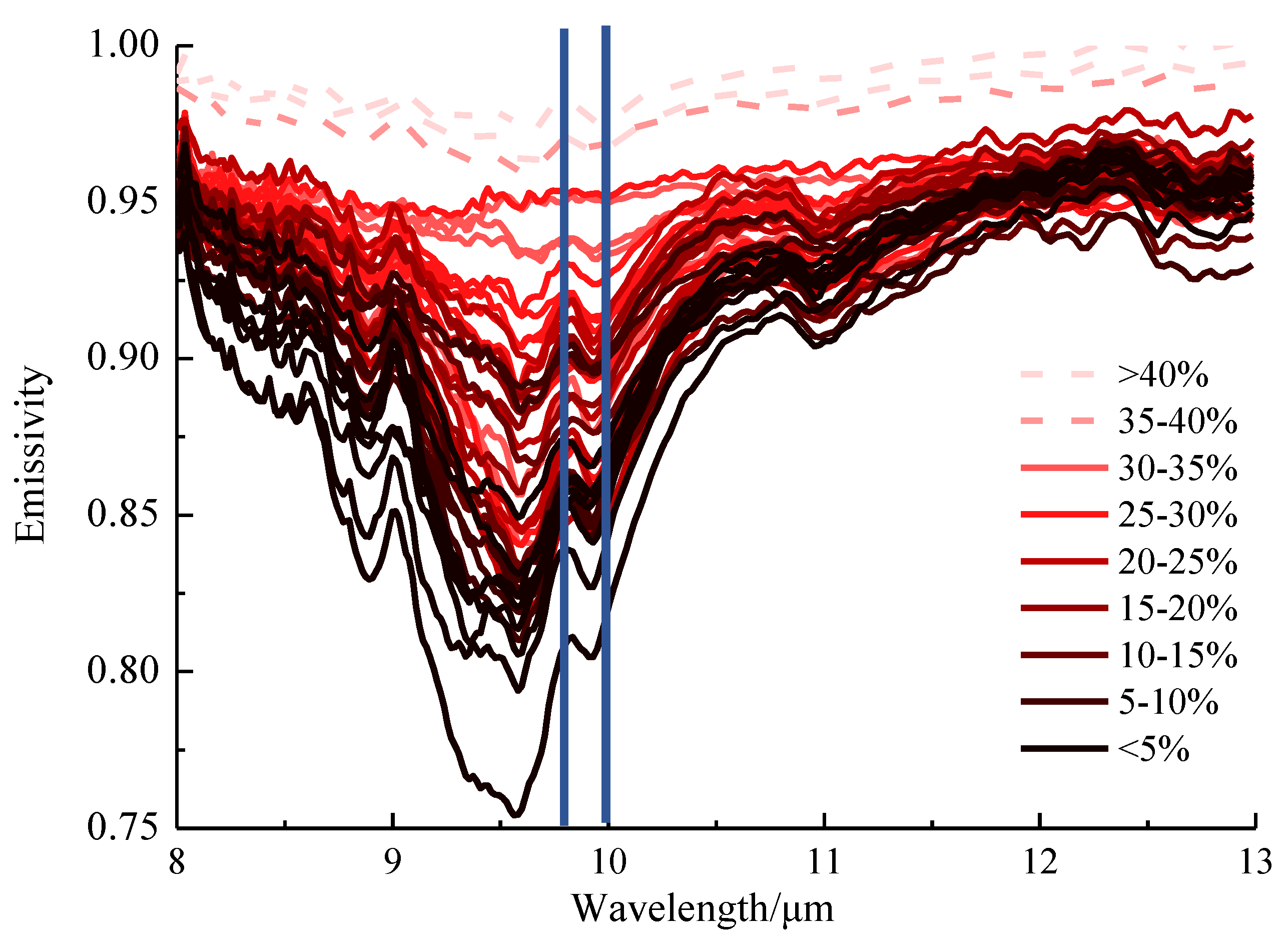
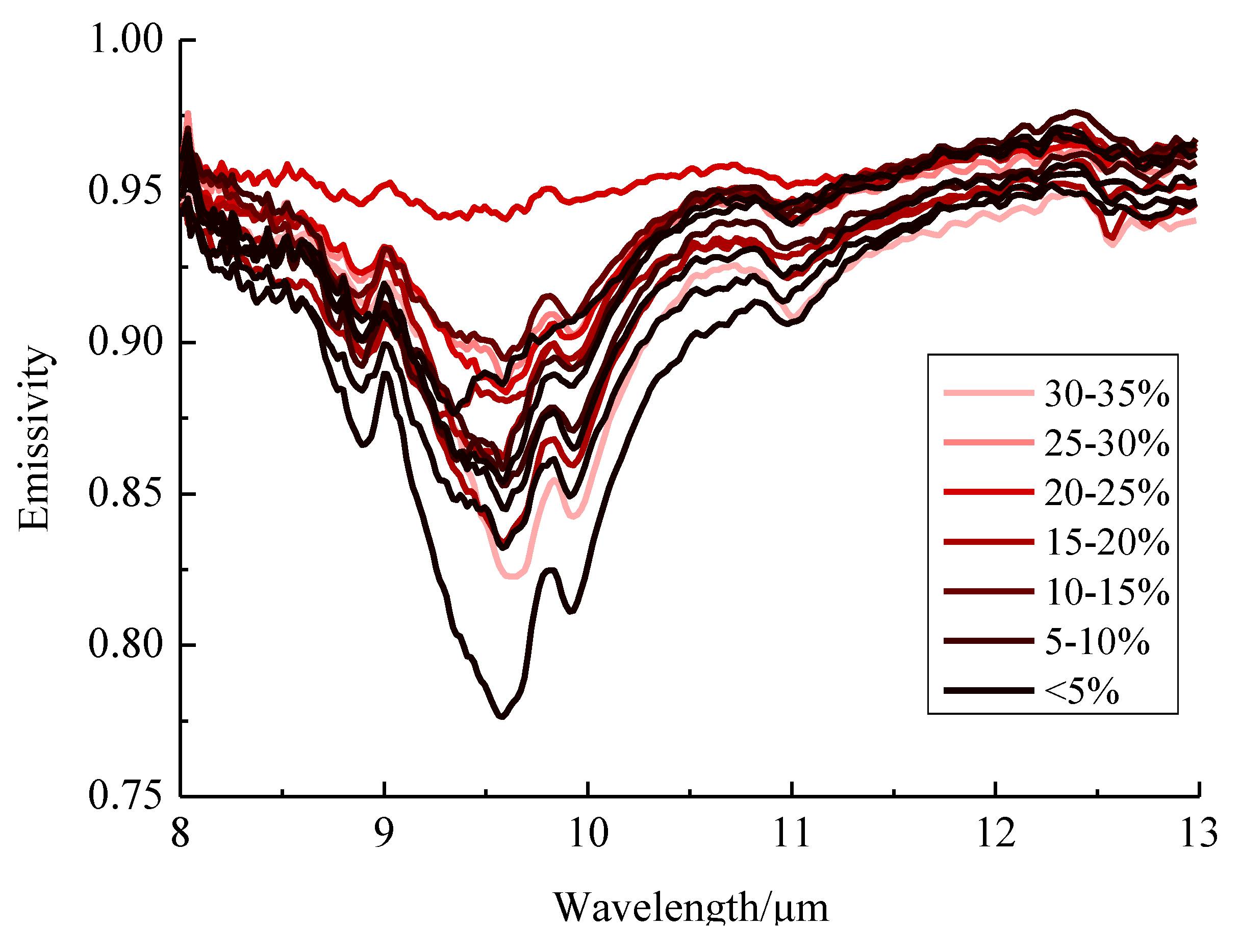
As the main mineral of coal gangue, carbon minerals have a thermal infrared spectrum curve close to 1, which is similar to the black body curve. Quartz, feldspar, mica and other silicate minerals have absorption characteristics at approximately 9.5 μm, which is mainly caused by Si-O bond vibration. As another major mineral of coal gangue, the thermal infrared spectrum of kaolinite has absorption characteristics at 9.5 μm and a trough characteristic at 10 μm, and the spectral features are consistent with that of the coal gangue samples.

When the content of carbonaceous minerals and kaolinite in the coal gangue samples is very high, a strong negative correlation is observed between the contents of the two minerals. Therefore, it is also feasible to predict the fixed carbon content of coal gangue based on the thermal infrared spectral characteristics of kaolinite.

4.2. Limitations

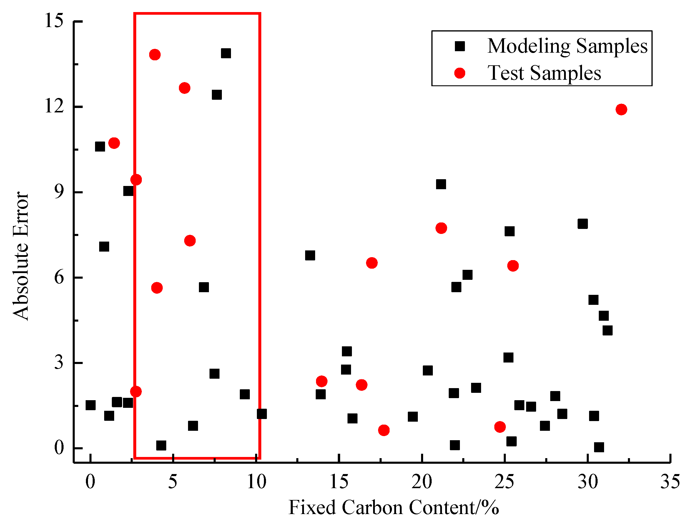
Although the overall prediction accuracy of the model is high, certain issues remain to be further addressed. The absolute error of the modeling samples and test samples has been analyzed as shown in Figure 9.

As shown in Figure 9, when the fixed carbon content of the sample is low (less than 10%), the prediction accuracy is poor. The main reason is that in this case, except for carbonaceous minerals and kaolinite, the contents of other mineral components are relatively large. At this time, the negative correlation between kaolinite content and carbonaceous mineral content is poor, therefore, the inversion of the fixed carbon content in coal gangue has greater errors based on the spectral characteristics of kaolinite.

We plan to introduce a deep learning algorithm to solve this problem in the next step. As a new machine learning algorithm, deep learning can better mine the effective information between data by characterizing the data and may represent a more efficient method of improving the inversion accuracy of coal gangue samples with a lower fixed carbon content. However, this method requires a large amount of sample data; therefore, we will further expand the sample size. We hope that the inversion accuracy can be improved via deep learning.

5. Conclusions

In this paper, a linear model based on the characteristics of thermal infrared spectra at the calculated sensitive bands is proposed to quantify the fixed carbon content of carbon gangue. The following conclusions are obtained:

(1)

The thermal infrared spectral characteristics of carbonaceous gangue are obviously different from those of coal samples, and the content of fixed carbon in gangue is closely related to the trough characteristics on the emissivity curve.

(2)

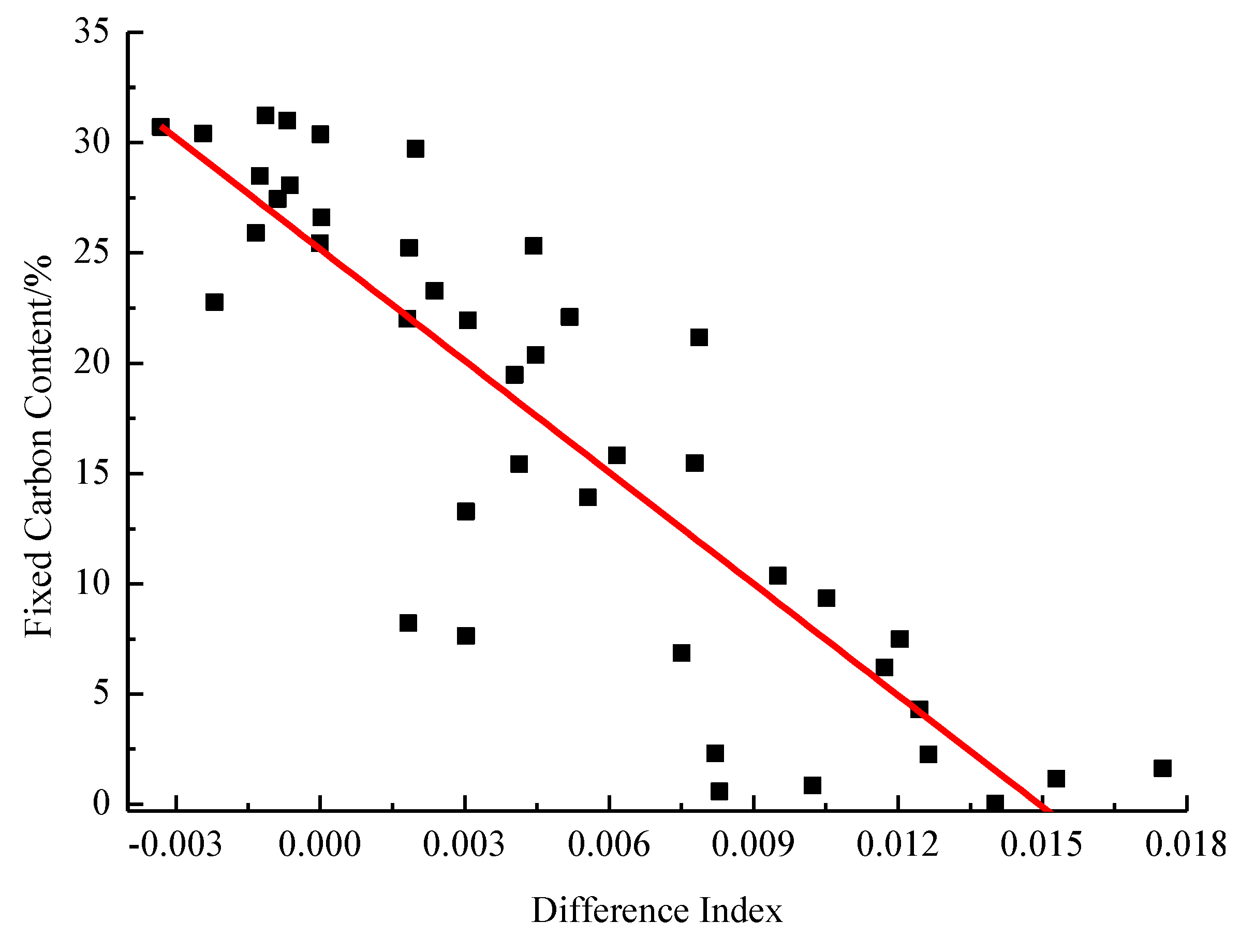
Based on the thermal infrared spectral characteristics, the difference index is strongly correlated with the fixed carbon content of the samples, and it presents a correlation coefficient of 0.8668. The linear model between the sensitive band difference index and the fixed carbon content is established.

(3)

Compared with the model prediction results of absorption depth, spectral absorption area, and the random forest and support vector machine algorithms, the proposed inversion model of fixed carbon content based on the difference index performs the best, and presents an average error of 5.00% for all samples and a root mean square error of 6.70. The results showed that the prediction accuracy of the model is high; thus, it can be applied to the prediction of fixed carbon content in coal gangue.

Data mining methods (RF, SVM, etc.) have obvious advantages when the sample size is sufficient. However, the proposed method has higher prediction accuracy in the case of small samples. Studies to quantify the fixed carbon of coal gangue present a long experimental process is long, and high test costs; therefore, generating a large amount of data is difficult. Therefore, the proposed method has more obvious advantages in coal mine applications.

Compared with chemical methods, this method has the advantages of being economic, rapid and efficient. The study in this paper provides an online monitoring method for the fixed carbon content of coal gangue. If the thermal spectroscopy of the discharged coal gangue can be tested, then the coal gangue can be finely discharged according to the fixed carbon level and further effectively utilized. This method not only effectively reduces the possibility of spontaneous combustion of coal gangue but also creates better economic benefits. These results are important to the environmental protection and safety of mines.

References

1. Bian, Z.F.; Dong, J.H.; Lei, S.G.; Leng, H.L.; Mu, S.G.; Wang, H. The impact of disposal and treatment of coal mining wastes on environment and farmland. Environ. Geol. 2009, 58, 625–634. [Google Scholar] [CrossRef]
2. Ribeiro, J.; da Silva, E.F.; Flores, D. Burning of coal waste piles from Douro Coalfield (Portugal): Petrological, geochemical and mineralogical characterization. Int. J. Coal Geol. 2010, 81, 359–372. [Google Scholar] [CrossRef]
3. Sun, Y.Z.; Fan, J.S.; Qin, P.; Niu, H.Y. Pollution extents of organic substances from a coal gangue dump of Jiulong Coal Mine, China. Environ. Geochem. Health 2009, 31, 81–89. [Google Scholar] [CrossRef]
4. Li, J.B.; Xian, X.F.; Mao, F.; Li, J.C. The Stability Evaluation of coal waste dump: Case of a chongqing coal mine. Disaster Adv. 2010, 3, 536–540. [Google Scholar]
5. Liang, T.S.; Zhang, Z.J. Blasting law and inducing factors of self-combustion waste heap. J. China Coal Soc. 2009, 34, 74–78. (In Chinese) [Google Scholar] [CrossRef]
6. Ribeiro, J.; Isabel, S.-R.; Flores, D. Geochemistry of self-burning coal mining residues from El Bierzo Coalfield (NW Spain): Environmental implications. Int. J. Coal Geol. 2016, 159, 155–168. [Google Scholar] [CrossRef]
7. Nádudvari, A.; Fabiańska, M.J. The impact of water-washing, biodegradation and self-heating processes on coal waste dumps in the Rybnik Industrial Region (Poland). Int. J. Coal Geol. 2016, 155, 286–299. [Google Scholar] [CrossRef]
8. Chugh, Y.P.; Patwardhan, A. Mine-mouth power and process steam generation using fine coal waste fuel. Resour. Conserv. Recyc. 2004, 40, 225–243. [Google Scholar] [CrossRef]
9. Pallares, J.; Herce, C.; Bartolom, C.; Pena, B. Investigation on co-firing of coal mine waste residues in pulverized coal combustion systems. Energy 2017, 140, 58–68. [Google Scholar] [CrossRef]
10. Taha, Y.; Benzaazoua, M.; Hakkou, R.; Mansori, M. Coal mine wastes recycling for coal recovery and eco-friendly bricks production. Miner. Eng. 2017, 107, 123–138. [Google Scholar] [CrossRef]
11. Czajka, K.M. Proximate analysis of coal by micro-TG method. J. Anal. Appl. Pyrol. 2018, 133, 82–90. [Google Scholar] [CrossRef]
12. Li, P.S.; Wang, Q.; Xu, Q.; Yu, W.; Yue, Y.N.; Liang, Z.; Dong, X.C.; Hu, S. Combustion reaction mechanism of four typical Chinese biomass by TG and DTG. Asia-Pac J. Chem. Eng. 2012, 7, S209–S215. [Google Scholar] [CrossRef]
13. Yu, D.X.; Xu, M.H.; Sui, J.; Liu, X.W.; Yu, Y.; Cao, Q. Effect of coal particle size on the proximate composition and combustion properties. Thermochim. Acta 2005, 439, 103–109. [Google Scholar] [CrossRef]
14. Gomez, Y.R.; Hernandez, R.C.; Guerrero, J.E.; Mejia-Ospino, E. FTIR-PAS coupled to partial least squares for prediction of ash content, volatile matter, fixed carbon and calorific value of coal. Fuel 2018, 226, 536–544. [Google Scholar] [CrossRef]
15. Posom, J.; Sirisomboon, P. Evaluation of the higher heating value, volatile matter, fixed carbon and ash content of ground bamboo using near infrared spectroscopy. J. Near Infrared Spec. 2017, 25, 301–310. [Google Scholar] [CrossRef]
16. Xue, J.J.; Yang, Z.L.; Han, L.J.; Liu, Y.C.; Liu, Y.; Zhou, C.C. On-line measurement of proximates and lignocellulose components of corn stover using NIRS. Appl. Energy 2015, 137, 18–25. [Google Scholar] [CrossRef]
17. Le, B.T.; Xiao, D.; Mao, Y.C.; He, D.K. Coal analysis based on visible-infrared spectroscopy and a deep neural network. Infrared Phys. Technol. 2018, 93, 34–40. [Google Scholar] [CrossRef]
18. Kim, D.W.; Lee, O.M.; Kim, J.S. Application of near infrared diffuse reflectance spectroscopy for on-line measurement of coal properties. Korean J. Chem. Eng. 2009, 26, 489–495. [Google Scholar] [CrossRef]
19. Xie, Y.; Li, F.Y.; Fan, X.J.; Hu, S.J.; Xiao, X.; Wang, J.F. Components Analysis of Biochar Based on Near Infrared Spectroscopy Technology. Chin. J. Anal. Chem. 2018, 46, 609–615. [Google Scholar] [CrossRef]
20. Yao, S.C.; Mo, J.H.; Zhao, J.B.; Li, Y.S.; Zhang, X.; Lu, W.Y.; Lu, Z.M. Development of a Rapid Coal Analyzer Using Laser-Induced Breakdown Spectroscopy (LIBS). Appl. Spectrosc. 2018, 72, 1225–1233. [Google Scholar] [CrossRef] [Green Version]
21. Yang, E.; Ge, S.R.; Wang, S.B. Characterization and Identification of Coal and Carbonaceous Shale Using Visible and Near-Infrared Reflectance Spectroscopy. J. Spectrosc. 2018. [Google Scholar] [CrossRef]
22. Xu, L.; Wang, Q. Retrieval of Soil Water content in saline soils from emitted thermal infrared spectra using partial linear squares regression. Remote Sens. 2015, 7, 14646–14662. [Google Scholar] [CrossRef]
23. Sawuta, M.; Ghulama, A.; Tiyipb, T.; Zhang, Y.J.; Ding, J.L.; Zhang, F.; Maimaitiyiming, M. Estimating soil sand content using thermal infrared spectra in arid lands. Int. J. Appl. Earth Obs. Geoinf. 2014, 33, 203–210. [Google Scholar] [CrossRef]
24. Xia, J.; Tiyipl, T.; Sawut, M.; Zhang, F.; Han, G.H. Application study of the thermal infrared emissity spectra in the estimation of salt content of saline soil. Spectrosc. Spectr. Anal. 2012, 32, 2956–2961. (In Chinese) [Google Scholar] [CrossRef]
25. Pascucci, S.; Casa, R.; Belviso, C.; Palombo, A.; Pignatti, S.; Castaldi, F. Estimation of soil organic carbon from airborne hyperspectral thermal infrared data: A case study. Eur. J. Soil. Sci. 2015, 65, 865–875. [Google Scholar] [CrossRef]
26. Hou, Y.J.; Tiyipl, T.; Zhang, F.; Sawut, M.; Nurmemet, I. Study on estimation of deserts soil total phosphorus content from thermal-infrared emissivity. Spectrosc. Spectr. Anal. 2015, 35, 350–354. (In Chinese) [Google Scholar] [CrossRef]
27. Yang, H.; Zhang, L.F.; Huang, Z.Q.; Zhang, X.W.; Tong, Q.X. Quantitative inversion of rock SiO2 content based on thermal infrared emissivity spectrum. Spectrosc. Spectr. Anal. 2012, 32, 1611–1615. (In Chinese) [Google Scholar] [CrossRef]
28. Zhang, L.F.; Zhang, X.W.; Huang, Z.Q.; Yang, H.; Zhang, F.Z. Quantitative estimation of CaO content in surface rocks using hyperspectral thermal infrared emissivity. Spectrosc. Spectr. Anal. 2011, 31, 2940–2943. (In Chinese) [Google Scholar] [CrossRef]
29. Feng, J.L.; Rivard, B.; Gallie, E.A.; Sandchez, A. Quantifying total sulfide content of cores and cut-rock surfaces using thermal infrared reflectance. Geophysics 2006, 71, 1–9. [Google Scholar] [CrossRef]
30. Salisbury, J.W.; Basu, A.; Fischer, E.M. Thermal infrared spectra of lunar soils. Icarus 1997, 130, 125–139. [Google Scholar] [CrossRef]
31. Hanna, K.L.D.; Greenhagen, B.T.; Patterson, W.R., III; Pieters, C.M.; Mustard, J.F.; Bowles, N.E.; Paige, D.A.; Glotch, T.D.; Thompson, C. Effects of varying environmental conditions on emissivity spectra of bulk lunar soils: Application to Diviner thermal infrared observations of the Moon. Icarus 2017, 283, 326–342. [Google Scholar] [CrossRef]
32. Koeppen, W.C.; Hamilton, V.E. Global distribution, composition, and abundance of olivine on the surface of Mar from thermal infrared data. J. Geophy. Res. 2008, 113, 1–23. [Google Scholar] [CrossRef]
33. Ramsey, M.S.; Harris, A.J.L.; Crown, D.A. What can thermal infrared remote sensing of terrestrial volcanoes tell us about processes past and present on Mars? J. Volcanol. Geotherm. Res. 2016, 311, 198–216. [Google Scholar] [CrossRef]
34. Hamilton, V.E. Thermal infrared (vibrational) spectroscopy of Mg–Fe olivines: A review and applications to determining the composition of planetary surfaces. Chem. Erde-Geochem. 2010, 70, 7–33. [Google Scholar] [CrossRef]
35. Fan, G.W.; Zhang, D.S.; Wang, X.F. Reduction and utilization of coal mine waste rock in China: A case study in Tiefa coalfield. Resour. Conserv. Recyc. 2014, 83, 24–33. [Google Scholar] [CrossRef]
36. Song, L.; Liu, S.J.; Yu, M.L. A classification method based on the combination of visible, near-infrared and thermal infrared spectrum for coal and gangue distinguishment. Spectrosc. Spectr. Anal. 2017, 37, 416–422. [Google Scholar]
37. Gillespie, A. Land Surface Emissivity. In Encyclopedia of Remote Sensing; Njoku, E.G., Ed.; Springer: New York, NY, USA, 2014; pp. 303–311. ISBN 978-0-387-36698-2. [Google Scholar]
38. Christensen, P.R.; Bandfield, J.L.; Hamilton, V.E.; Howard, D.A.; Lane, M.D.; Piatek, J.L.; Ruff, S.W.; Stefanov, W.L. A thermal emission spectral library of rock-forming minerals. J. Geophys. Res. 2000, 105, 9735–9739. [Google Scholar] [CrossRef] [Green Version]
39. McFeeters, S.K. The use of Normalized Difference Water Index (NDWI) in the delineation of open water features. Int. J. Remote Sens. 1996, 17, 1425–1432. [Google Scholar] [CrossRef]
40. Zha, Y.; Gao, J.; Ni, S. Use of normalized difference built-up index in automatically mapping urban areas from TM imagery. Int. J. Remote Sens. 2003, 24, 583–594. [Google Scholar] [CrossRef]
41. Hong, Y.S.; Zhu, Y.X.; Su, X.P.; Zhu, Q.; Zhou, Y.; Yu, L. Estimation of soil organic matter content using hyperspectral techniques combined with normalized difference spectral index. Spectrosc. Spectr. Anal. 2017, 37, 3537–3542. (In Chinese) [Google Scholar] [CrossRef]
42. Bouzekri, S.; Lasbet, A.A.; Lachehab, A. A New Spectral Index for Extraction of Built-Up Area Using Landsat-8 Data. J. Indian Soc. Remote Sens. 2015, 43, 867–873. [Google Scholar] [CrossRef]
43. Zhang, Q.; Huang, W.J.; Cui, X.M.; Shi, Y.; Liu, L.Y. New Spectral Index for Detecting Wheat Yellow Rust Using Sentinel-2 Multispectral Imagery. Sensors 2018, 18, 868. [Google Scholar] [CrossRef]
44. Dillner, A.M.; Takahama, S. Predicting ambient aerosol thermal-optical reflectance (TOR) measurements from infrared spectra: Organic carbon. Atmos. Meas. Technol. 2015, 8, 4013–4023. [Google Scholar] [CrossRef]
45. Diamantidis, N.A.; Karlis, D.; Giakoumakis, E.A. Unsupervised stratification of cross-validation for accuracy estimation. Artif. Intell. 2000, 116, 1–16. [Google Scholar] [CrossRef] [Green Version]
46. Breiman, L. Random Forests. Mach. Learn. 2001, 45, 5–32. [Google Scholar] [CrossRef] [Green Version]
47. Gambill, D.R.; Wall, W.A.; Fulton, A.J.; Howard, H.R. Predicting USCS soil classification from soil property variables using Random Forest. J. Terramech. 2016, 65, 85–92. [Google Scholar] [CrossRef]
48. Vapnik, V.N. Satistical Learning Theory; Wiley-Interscience: New York, NY, USA, 1998; pp. 401–440. ISBN 0-471-03001-1. [Google Scholar]
49. Chapelle, O.; Vapnik, V.; Bousquet, O.; Mukherjee, S. Choosing Multiple Parameters for Support Vector Machines. Mach. Learn. 2002, 46, 131–159. [Google Scholar] [CrossRef] [Green Version]
50. Zhang, H.; Wu, P.B.; Yin, A.J.; Yang, X.H.; Zhang, M.; Gao, C. Prediction of soil organic carbon in an intensively managed reclamation zone of eastern China: A comparison of multiple linear regressions and the random forest model. Sci. Total Environ. 2017, 529, 704–713. [Google Scholar] [CrossRef]
51. Mutanga, O.; Adam, E.; Cho, M.A. High density biomass estimation for wetland vegetation using WorldView-2 imagery and random forest regression algorithm. Int. J. Appl. Earth Obs. Geoinf. 2012, 18, 399–406. [Google Scholar] [CrossRef]
52. Hu, X.F.; Belle, J.H.; Meng, X.; Wlidani, A.; Waller, L.A.; Strickland, M.J.; Liu, Y. Estimating PM2.5 Concentrations in the Conterminous United States Using the Random Forest Approach. Environ. Sci. Technol. 2017, 51, 6936–6944. [Google Scholar] [CrossRef]
53. Chauchard, F.; Cogdill, R.; Roussel, S.; Roger, J.M.; Bellon-Maurel, V. Application of LS-SVM to non-linear phenomena in NIR spectroscopy: Development of a robust and portable sensor for acidity prediction in grapes. Chemometr. Intell. Lab. 2004, 71, 141–150. [Google Scholar] [CrossRef]
54. Huang, M.W.; Chen, C.W.; Lin, W.C.; Ke, S.W.; Tsai, C.F. SVM and SVM Ensembles in Breast Cancer Prediction. PLoS ONE 2017, 12, e0161501. [Google Scholar] [CrossRef] [PubMed]
55. Thorpe, M.T.; Rogers, A.D.; Bristow, T.F.; Pan, C. Quantitative compositional analysis of sedimentary materials using thermal emission spectroscopy: 1. Application to sedimentary rocks. J. Geophy. Res. 2015, 120, 1956–1983. [Google Scholar] [CrossRef]
Figure 1. Photo of coal gangue dumps being used in the Tiefa mining area. (a) Unburned coal gangue dump, (b) burned coal gangue dump.
Energies 12 01659 g001
Figure 2. Diagram of the fixed carbon content of 42 gangue samples.
Energies 12 01659 g002
Figure 3. Visible, near-infrared spectrum of 42 coal gangues and three coal samples.
Energies 12 01659 g003
Figure 4. Thermal infrared spectra of 42 coal gangue and three coal samples.
Energies 12 01659 g004
Figure 5. (a) Correlation map of difference index (DI) and fixed carbon content; (b) correlation map of ratio index (RI) and fixed carbon content; and (c) correlation map of normalized difference index (NDI) and fixed carbon content.
Energies 12 01659 g005
Figure 6. Fitting results of the fixed carbon content and ratio index.
Energies 12 01659 g006
Figure 7. Thermal infrared spectra of the test samples.
Energies 12 01659 g007
Figure 8. Diagram of thermal infrared spectra of carbonaceous gangue samples.
Energies 12 01659 g008
Figure 9. Absolute error diagram of the modeled samples and test samples.
Energies 12 01659 g009