Article

Weighted Regression-Based Extremum Response Surface Method for Structural Dynamic Fuzzy Reliability Analysis

1
School of Aeronautics, Northwestern Polytechnical University, Xi’an 710072, China
2
Department of Aeronautics and Astronautics, Fudan University, Shanghai 200433, China
*
Author to whom correspondence should be addressed.
Energies 2019, 12(9), 1588; https://doi.org/10.3390/en12091588
Submission received: 3 April 2019 / Accepted: 23 April 2019 / Published: 26 April 2019

Abstract

:
The parameters considered in structural dynamic reliability analysis have strong uncertainties during machinery operation, and affect analytical precision and efficiency. To improve structural dynamic fuzzy reliability analysis, we propose the weighted regression-based extremum response surface method (WR-ERSM) based on extremum response surface method (ERSM) and weighted regression (WR), by considering the randomness of design parameters and the fuzziness of the safety criterion. Therein, we utilize the ERSM to process the transient to improve computational efficiency, by transforming the random process of structural output response into a random variable. We employ the WR to find the efficient samples with larger weights to improve the calculative accuracy. The fuzziness of the safety criterion is regarded to improve computational precision in the WR-ERSM. The WR-ERSM is applied to perform the dynamic fuzzy reliability analysis of an aeroengine turbine blisk with the fluid-structure coupling technique, and is verified by the comparison of the Monte Carlo (MC) method, equivalent stochastic transformation method (ESTM) and ERSM, with the emphasis on model-fitting property and simulation performance. As revealed from this investigation, (1) the ERSM has the capacity of processing the transient of the structural dynamic reliability evaluation, and (2) the WR approach is able to improve modeling accuracy, and (3) regarding the fuzzy safety criterion is promising to improve the precision of structural dynamic fuzzy reliability evaluation, and (4) the change rule of turbine blisk structural stress from start to cruise for the aircraft is acquired with the maximum value of structural stress at t = 165 s and the reliability degree (Pr = 0.997) of turbine blisk. The proposed WR-ERSM can improve the efficiency and precision of structural dynamic reliability analysis. Therefore, the efforts of this study provide a promising method for structural dynamic reliability evaluation with respect to working processes.

1. Introduction

In mechanical systems, the structures always endure complex loads in the extreme environment. For instance, an aeroengine turbine blisk always suffers from high temperature, high pressure and high speed under operation [1]. With the increasing complexity of a mechanical system, the requirements on structural design have become higher. A structural failure during operation could seriously threaten the safety of the entire system and could even be catastrophic. Therefore, it is worthwhile to perform reliability analysis to improve the performance of mechanical system.
In respect of a large number of investigations on the structural reliability evaluations, many methods were developed and briefly described below. Liu et al. [2] adopted a first-order reliability method (FORM) in the chatter reliability analysis of milling system. Keshtegar [3] used the hybrid conjugate search direction to improve the efficiency and robustness of FORM in structural reliability analysis. Zhang et al. [4] proposed a second-order reliability method (SORM) for mechanical reliability design. Huang et al. [5] developed a new SORM with saddlepoint approximation for reliability analysis. Hu et al. [6] explored a novel second order approximation for structural reliability analysis. Nakamura et al. [7] discussed the Monte Carlo (MC) method by the probabilistic transient thermal analysis of an atmospheric reentry vehicle structure. Martinez-Velasco et al. [8] studied the reliability of distribution systems with distributed generation using the parallel MC method. Yang et al. [9] evaluated the structural reliability of a beam pumping unit by the finite element (FE) method with the MC simulation. However, it is difficult to employ FORM and SORM in complicated calculations in structural reliability analysis for low computing accuracy. Moreover, the MC method always spends tremendous time on structural reliability analysis for the requirement of a large number of iterations and simulations.
To address the above issues, surrogate models (called response surface methods, RSM) emerged and underwent rapid development. So far, various surrogate models have been appeared, such as RSM-based polynomials, Kriging model, neural network method, support vector machine, and so forth. Yang et al. [10] used the RSM and FE model to optimize preform shapes, to improve deformation homogeneity in aerospace forgings. Allaix and Carbone [11] proposed the coupling method of the RSM and FE method for structural reliability analysis to prohibit computational cost. In the above works, the RSM has been validated to hold higher computational efficiency than the MC simulation. However, it is troublesome to apply the RSM to process the nonlinearity and transient problems of complex structural reliability analyses, because it is impossible for the RSM model to perfectly reflect the parameter features in high-dimensional space and thus ensure modeling precision. In this case, the Kriging model was developed by Danie G. Krige (after whom the method is named), and then also applied in the field of structural reliability [12,13]. As a classical implicit and intelligent algorithm, the neural network method was investigated in structural reliability analyses [14,15]. Additionally, a support vector machine is also widely focused on since the outstanding performance in overcoming high-dimensional and nonlinear features in structural reliability [16,17]. Although these methods have acceptable accuracy in modeling and reliability assessment in static reliability analysis, it is difficult for these methods to accurately evaluate structural dynamic reliability with time-varying features and the increasing limit state functions.
With respect to the solution of the above questions, extremum RSM (ERSM) was first proposed to handle the transient problem of two-link flexible rotor manipulator reliability analysis, by regarding the time-varying feature and the extremum values of output responses [18]. Later, the ERSM was extended to the dynamic probabilistic designs of aeroengine typical components such as disks and blades [19,20]. The investigations revealed that the ERSM is efficient to reduce computational burden in structural dynamic reliability design to some extent. As for the transients and nonlinearity of structural dynamic reliability analyses, however, the ERSM still face with the low and even unacceptable computational accuracy. In addition, the use of the parameters always influences the modeling precision. In the improvement of modeling accuracy, the weighted regression (WR) is an efficient way by seeking for the better values of the parameters in modeling. Broadie et al. [21] improved the risk estimation model of a financial budget via the WR. The WR technique was also applied to the surrogate modeling of structural reliability analyses. Kaymaz and McMahon [22] utilized the WR to improve the response surface model. In the related published works, it has not been found that the technique is employed in structural dynamic reliability analysis. Along with the heuristic thought, we apply the WR to structural dynamic reliability analysis to refine the modeling precision and accuracy. Meanwhile, the strong fuzziness of parameters is ubiquitous in the material property, boundary conditions, geometry sizes, safety criteria, and so forth [23,24,25]. Herein, the safety criterion is fuzzy when a specific failure value cannot be determined. The fuzzy safety criterion is more reasonable in structural fuzzy reliability analyses, because the analytical accuracy is improved by transforming fuzzy safety criterion to stochastic safety criterion [26,27,28].
To perform a structural dynamic reliability analysis with high-precision, this study proposes an efficient approach based on the ERSM and WR, called as WR-based ERSM (WR-ERSM), to improve the accuracy of surrogate modeling and reliability analysis. In the WR-ERSM, the ERSM is employed to address the transient problem of structural dynamic reliability analysis by simplifying the stochastic process of output response as a random variable, the WR is introduced to find the efficient samples for the ERSM modeling to improve modeling accuracy, and the fuzziness of the safety criterion is considered to improve the precision of dynamic reliability analysis by transforming fuzzy safety criterion into stochastic safety criterion. The proposed WR-ERSM is validated by the dynamic fuzzy reliability analysis of a turbine blisk with regard to both the randomness of input variables and the fuzziness of safety criterion.
In Section 2 WR-ERSM is developed for structural dynamic fuzzy reliability analysis. Section 3 investigates the dynamic fuzzy reliability analysis of an aeroengine turbine blisk based on the WR-ERSM by considering fluid-structure interaction and fuzzy safety criterion. The developed WR-ERSM is validated by the comparison of methods in Section 4. The conclusions on this study are summarized in Section 5.

2. Basic Theory on Dynamic Fuzzy Reliability Analysis

In this section, we discuss the basic principle of the WR-ERSM for structural dynamic fuzzy reliability analysis as drawn in Figure 1.
As revealed in Figure 1, the process of structural dynamic fuzzy reliability analysis comprises analytical preparation, WR-ERSM modeling, sample extraction, safety criterion transformation and reliability analysis. The analytical preparation is to structure finite model (FE) model and set all constraint conditions, workloads and time domain. The objective of the samples’ extraction is to collect all input and output samples from dynamic deterministic analyses as one pool of samples for dynamic probabilistic analysis. Herein, the samples of random inputs are extracted by the full factorial design [29,30], and then the extrema of response processes are gained as new output responses based on dynamic deterministic analysis in the time domain of interest, and their weights are confirmed by a series of deterministic analyses with the acquired input samples and FE model. In the process of WR-ERSM modeling, the samples with larger weights, which include input samples and output samples, are chosen from the pool of samples as the fitting samples for the WR-ERSM modeling. When the fitting accuracy does not satisfy the requirements, the fitting samples are reselected to achieve the weighted values. Otherwise, the probability density functions (PDFs) of outputs are gained by MC method. The objective of safety criterion transformation is to transform the fuzzy safety criterion into a stochastic safety criterion based on the fuzzy entropy principle [31,32]. Lastly, structural dynamic fuzzy reliability analysis is performed to achieve the reliability degree considering the randomness of input variables and the fuzziness of safety criterion.

2.1. Weighted Regression Extremum Response Surface Method (WR-ERSM) Modeling

The ERSM was developed to evaluate structural dynamic reliability by considering the extremum values instead of all the output responses within the time domain of interest, and was proved to be efficient in terms of the efficiency improvement [18,33]. In other words, the random process of an output response in the time domain is transformed into a random variable as the ERSM is modeled. When y(x) denotes the extremum of output response within the time domain [0, T], corresponding to the input variables x = [x1, x2, …, xk]T, where k is the number of inputs, the ERSM model can be expressed as:
y ( x ) = A + B x + x T C x
in which A, B and C indicate constant term, linear term and quadratic term. B and C are denoted as:
{ B = [ b 1 , b 2 , , b k ] C = ( c 1 0 0 c k )
here i = 1, 2, …, k. Thus, the ERSM function can be rewritten as:
y ( x ) = a + i = 1 k b i x i + i = 1 k c i x i 2
In this equation, the number of undetermined coefficients is 2k + 1. To compute these coefficients, we extract a series of input samples by the full factorial design method in Equation (4).
E 1 = ( μ 1 , μ 2 , , μ k ) E 2 = ( μ 1 , μ 2 , , μ i ± f σ i , , μ k ) E 3 = ( μ 1 , μ 2 , , μ i ± f σ i , , μ j ± f σ j , , μ k ) E s = ( μ 1 ± f σ 1 , μ 2 ± f σ 2 , , μ i ± f σ i , , μ k ± f σ k )
where El (l = 1, 2, …, s) is the l-th sampling category, namely experimental condition, which is the rule of generated sample set of random variable with respect to both the mean μ and standard deviation σ; the subscripts i, j indicate the i-th and j-th random variables; the subscript s expresses the number of sampling types; f denotes the empirical coefficient which is usually selected from 1 to 3.
Based on structural dynamic deterministic analysis and the least square method [1,19,34], the output responses are then acquired by Equation (5).
d = ( v T v ) 1 v T y v = [ 1 x 11 x 12 x 1 k x 11 2 x 12 2 x 1 k 2 1 x 21 x 22 x 2 k x 21 2 x 22 2 x 2 k 2 1 x n 1 x n 2 x n k x n 1 2 x n 2 2 x n k 2 ] d = [ a , b 1 , b 2 , , b k , c 1 , c 2 , , c k ]
The symbol v is the n × (k + 1) matrix of input variables, in which n is the number of samples; d is the vector of undetermined coefficients in the ERSM model.
In respect of the ERSM, the computational burden is effectively reduced in structural dynamic reliability evaluation. However, the modeling precision is still unacceptable because of the limitations of quadratic polynomials in processing the high non-linearity problem and large-scale parameters. To resolve this issue, this study develops the WR-ERSM with respect to the ERSM and WR. We adopt the ERSM to compute the global extreme value rather than all the values for the dynamic output responses under different input parameters in the time domain [0, T], and employ the WR to find the optimal parameters in the process of the ERSM modeling.
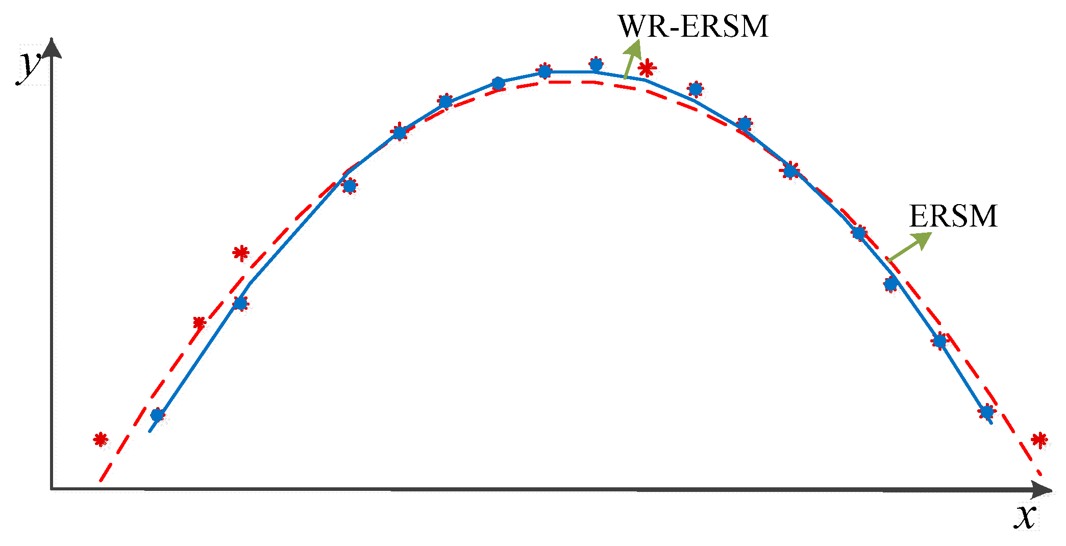
The comparison of the ERSM and the WR-ERSM are shown in Figure 2. The ERSM model (indicated by the red dotted curve) is established by all the samples based on the least square method. For the WR-ERSM modeling (denoted by the blue solid curve), we first apply the WR to select the efficient samples (annotated by the blue dots) with larger weights from the pool of n samples, to determine the undetermined coefficients and gain the WR-ERSM model. This method is termed the weighted least square method.
Regarding the ERSM model (Equation (1)), the WR-ERSM model yWR(x) is structured as:
y W R ( x ) = A W R + B W R x + x T C W R x
where AWR, BWR and CWR are the weighted constant, weighted linear vector and weighted quadratic matrix, respectively. BWR and CWR are denoted as
{ B W R = [ b W R , 1 , b W R , 2 , , b W R , k ] C W R = [ c W R , 1 c W R , 2 c W R , k ]
To intuitively express the WR-ERSM model, the Equation (6) is written as quadratic polynomial, i.e.,
y W R ( x ) = a W R + i = 1 k b W R , i x i + i = 1 k c W R , i x i 2
in which aWR, bWR,i and cWR,i are the weighted coefficient of A, B and C, respectively.
To determine these weighted coefficients in Equation (8), we first need to search the minimum of output responses yobj(x) with respect to n samples, the weighted values are then obtained by dividing the minimum value yobj(x) from all the output responses ytrue(x), which are ensured by dynamic deterministic analysis with the FE model. The m efficient samples with larger weights are selected from this pool of n samples, and the weighted matrix w is restructured. The related formulas are:
{ y o b j ( x ) = min | y t r u e , j ( x ) | w j = y o b j y t r u e , j ( x ) w = [ w 1 w m ]
here j = 1, 2, …, n; ytrue, j(x) indicates the true value of the j-th output response; wj is the weighted value of the j-th sample; m (m ≥ (2k + 1)) is the number of efficient samples.
We confirm the undetermined coefficients of WR-ERSM model, i.e.,
d W R = ( v W R T w v W R ) 1 v W R T w y W R
where dWR denotes the vector of undetermined coefficients in the WR-ERSM model; vWR is the matrix of efficient samples; yWR is the output response corresponding to the efficient samples. dWR, vWR and yWR are structured as:
{ d W R = [ a W R , b W R , 1 , b W R , 2 , b W R , k , c W R , 1 , c W R , 2 , c W R , k ] v W R = [ 1 x W R , 11 x W R , 12 x W R , 1 k x W R , 11 2 x W R , 12 2 x W R , 1 k 2 1 x W R , 21 x W R , 22 x W R , 2 k x W R , 21 2 x W R , 22 2 x W R , 2 k 2 1 x W R , m 1 x W R , m 2 x W R , m k x W R , m 1 2 x W R , m 2 2 x W R , m k 2 ] y = [ y ( x 1 ) , y ( x 2 ) , , y ( x n ) ] T
Based on the above analysis, we can derive the WR-ERSM model.

2.2. Safety Criterion Transformation

In engineering practice, most factors have stochastic and fuzzy characteristics. For structural dynamic reliability analysis, various methods have been developed so far to process the effect of the random parameters. However, those methods are unable to resolve the influences of the randomness and fuzziness simultaneously. As typical fuzzy factors, the allowable values, e.g., deformation, stress, strain, and so forth, of the safety criterion generally depend on experimental statistics. Actually, these parameters always vary in small range in engineering. Hence, it is more reasonable to consider the randomness of inputs and the fuzziness of safety criterion in structural dynamic reliability analysis.
To address this issue, we transform the fuzzy safety criterion into a random safety criterion in the structural dynamic fuzzy reliability evaluation. This paper deals with the fuzzy safety criterion by the fuzzy entropy principle, which has been validated to be feasible [31,32,35,36]. For transforming the fuzzy safety criterion into random safety criterion, we first determine the membership function of safety criterion distribution feature, which is generally chosen as a triangular membership function in engineering practice [23,28,36]. Hence, we also select a triangular membership function to describe the information for the safety criterion as shown in Equation (12).
u y ˜ ( x ) = { x a 1 a a 1 , a 1 < x a a 2 x a 2 a , a < x a 2 0 , otherwise
We can compute the mean and standard deviation of stochastic safety criterion with a normal distribution based on the fuzzy entropy principle in Equation (13), and then acquire the PDF of safety criterion:
μ e q = ( 1 + u y ˜ ( x ) d x ) + x u y ˜ ( x ) d x σ e q = 1 2 π exp ( G x 0.5 )
where μeq and σeq indicates the mean and standard deviation of equivalent random parameter; μ y ˜ ( x ) is the membership function of fuzzy safety criterion; Gx is defined as:
G x = + u y ˜ ( x ) ln u y ˜ ( x ) d x = u l u u u y ˜ ( x ) u l u u u y ˜ ( x ) d x ln u y ˜ ( x ) u l u u u y ˜ ( x ) d x d x
here uu and ul are the upper bound and lower bound of fuzzy variable interval, respectively.
Finally, the PDF of safety criterion is reshaped as:
f e q ( z e q ) = 1 2 π σ e q exp ( ( z e q μ e q ) 2 2 σ e q 2 )
Through the above analysis, we can transform the fuzzy safety criterion into a stochastic safety criterion by using the fuzzy entropy principle.

2.3. Structural Dynamic Fuzzy Reliability Analysis

To accomplish structural dynamic reliability analysis, we need to build the PDF of output. In this case, we take structural stress as analytical object (output response). Based on the derived WR-ERSM model in Equation (8), we extract a large number of samples of the output based on MC method, and achieve the mean and standard deviation. The formula of PDF is then established, i.e.,
f ( z ) = 1 2 π σ z exp ( ( z μ z ) 2 2 σ z 2 )
where z expresses the structural stress; μz and σz are both mean value and standard deviation, respectively.
With the PDF of safety criterion, the fuzzy reliability index β and reliability degree Pr of the complex structure are:
{ β = μ z μ e q σ z 2 + σ e q 2 P r = Φ ( β )
where μz and σz present the mean value and standard deviation of output response; μeq and σeq indicate the mean value and standard deviation of the safety criterion.

3. Example Analysis

In this section, we regarded the dynamic fuzzy reliability analysis of an aeroengine turbine blisk as one case to verify the feasibility and effectiveness of the proposed WR-ERSM algorithm.

3.1. Deterministic Analysis for Turbine Blisk

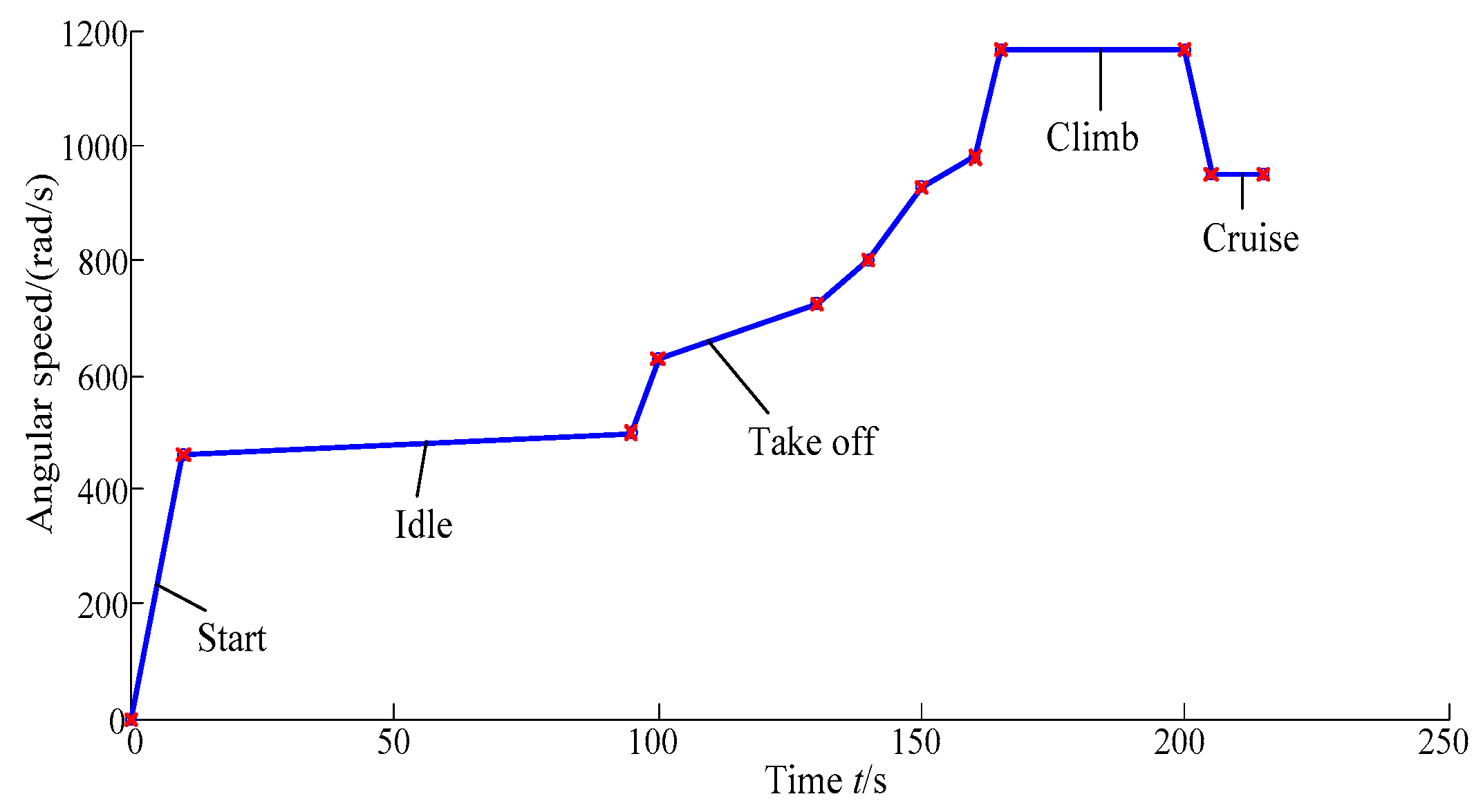
Working in the extreme environment, turbine blisk endures high temperature, high pressure and high speed. To simulate the variation of turbine blisk stress under different operation status, the analytical range of start, idle, take off, climb and cruise is selected from the flight profile of the aeroengine in the time domain [0 s, 215 s] [37,38]. In this time domain [0 s, 215 s], 12 critical points of angular speed shown in Figure 3 are selected during the aeroengine operation of time domain. In this study, nickel-base alloy is selected as the material of the gas turbine blisk.
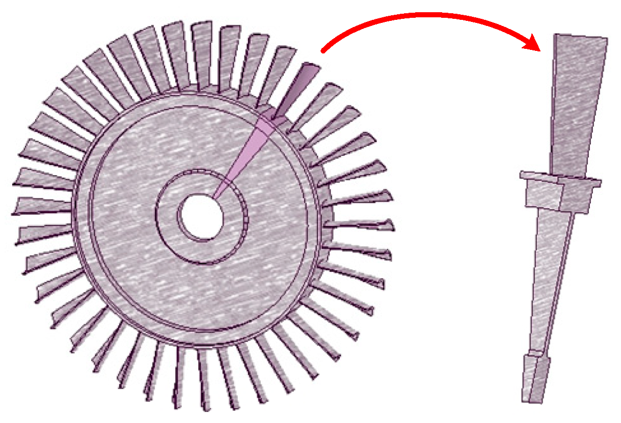
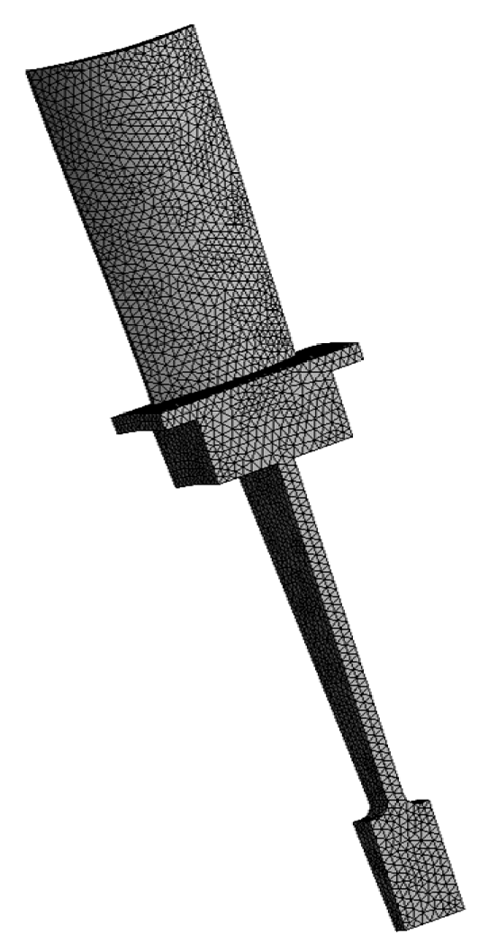
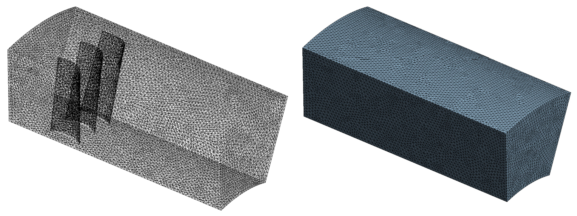
The turbine blisk is a typically cyclic symmetric structure comprising one disk and 40 blades, and is shown in Figure 4. To reduce the calculation burden, the 1/40 of the blisk model is regarded as the study object, besides the cooling holes on blisk are simplified. The FE models of the turbine blisk (29,332 elements and 47,933 nodes) and flow field (222,370 elements and 321,632 nodes) are shown in Figure 5 and Figure 6, respectively.
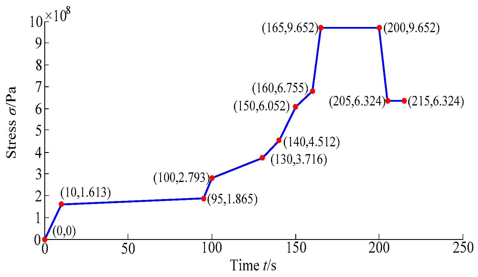
To simulate the variation of structural stress caused by fluid and structural loads within the time domain [0 s, 215 s], the dynamic deterministic analysis of the turbine blisk is fulfilled by both the close coupled analysis method and fluid–structure interaction [39,40,41]. The variation curve of turbine blisk stress in the time domain [0 s, 215 s] is displayed in Figure 7, in which σ is the stress of turbine blisk (similarly hereinafter).
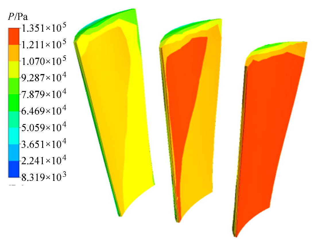
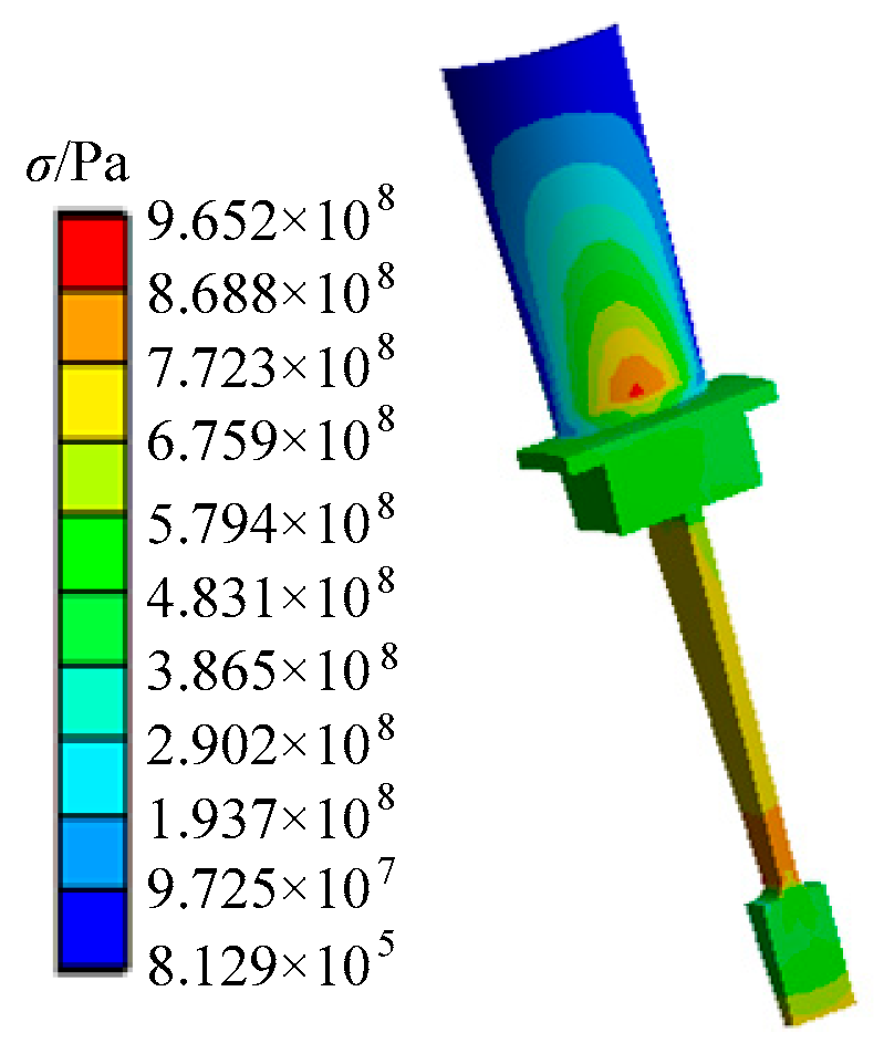
As revealed in Figure 7, the turbine blisk stress rises with the increasing angular speed. The maximum of stress emerges at t = 165 s in cruise phase. Thus, we regarded t = 165 s as the computational point of turbine blisk dynamic fuzzy reliability analysis. The nephograms of pressure and stress distributions on the fluid–structure coupling interface at t = 165 s are acquired in Figure 8 and Figure 9, in which P is the pressure on the fluid–structure coupling interface. As revealed in Figure 9, the maximum stress is at the root of the turbine blade.

3.2. The WR-ERSM Model of Turbine Blisk

To achieve the surrogate model of turbine blisk, the factors (parameters) impacting the analytical results are selected as the random input variables as listed Table 1, including inlet velocity, inlet pressure, material density and angular speed.
As revealed in Table 1, the mean μ of the random input variables is determined within the time domain by using the extremum selection method [42]. To establish the WR-ERSM model of turbine blisk, the samples are extracted from the random inputs and outputs at the selected calculation points by the full factorial design in Equation (4). The weighted values of output responses are calculated by Equation (5). The 40 samples are listed in Table 2.
Based on 20 groups of samples with larger weights underlined in Table 2, the coefficients of Equation (8) are acquired, and then the WR-ERSM model of turbine blisk is
y ( x ) = 2.746 × 10 9 + 2.258 × 10 6 x 1 9.681 × 10 2 x 2 + 1.063 × 10 5 x 3 + 3.053 × 10 6 x 4 7.036 × 10 3 x 1 2 + 8.078 × 10 4 x 2 2 + 0.418 x 3 2 4.722 × 10 2 x 4 2
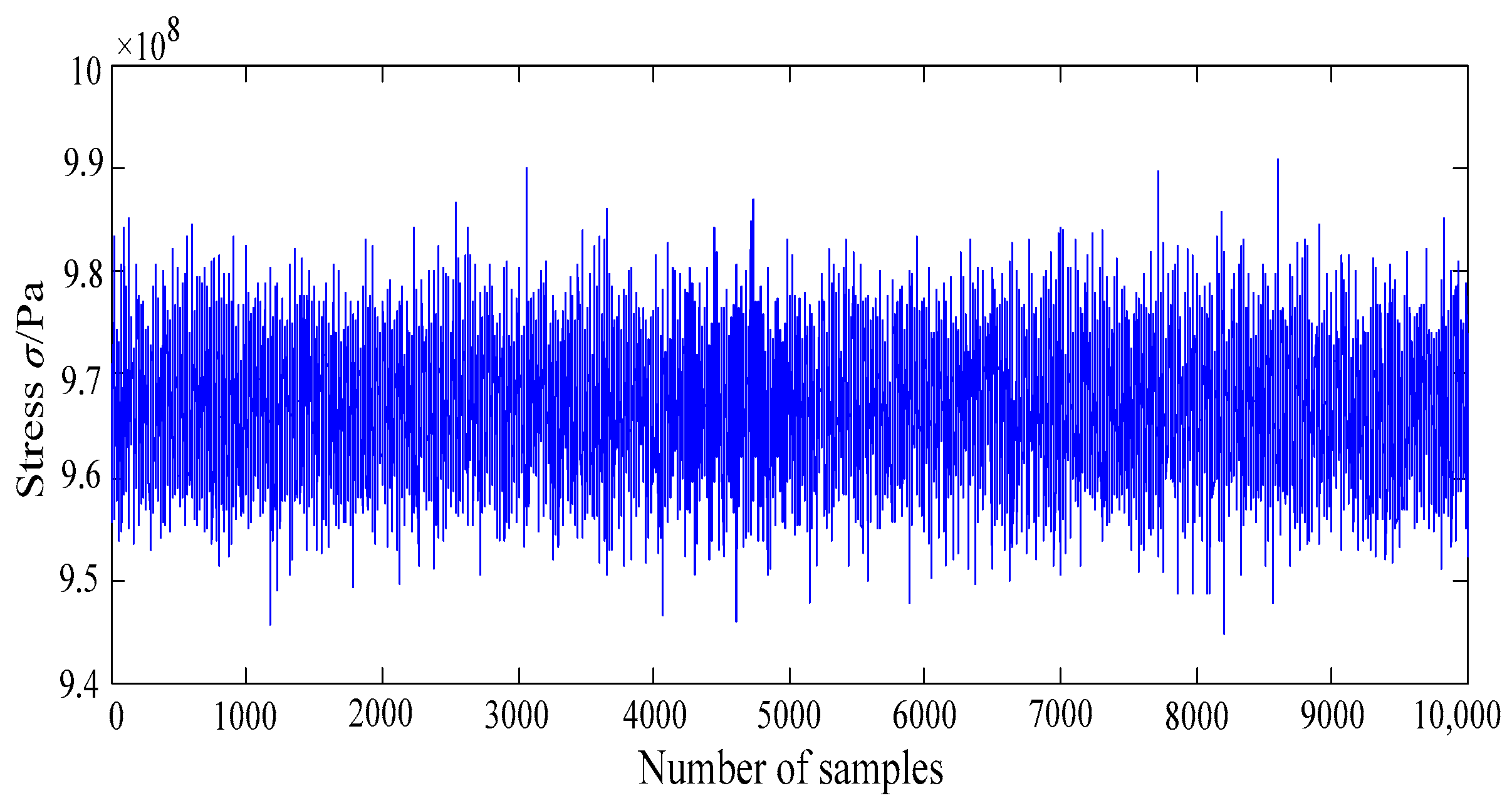
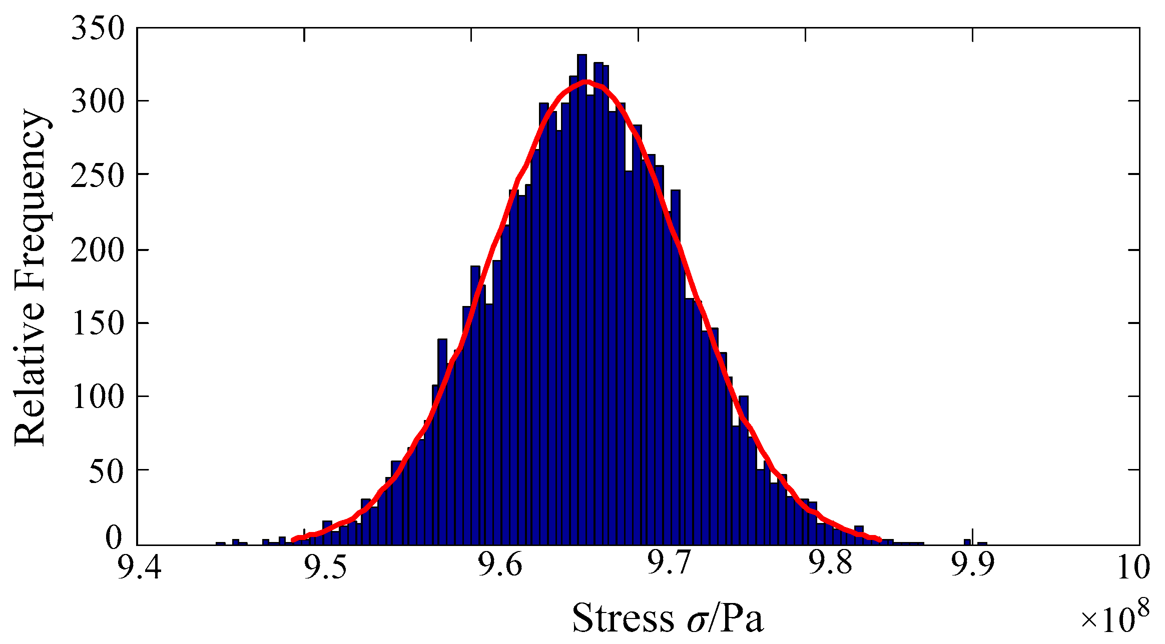
Let the response y(x) in Equation (18) obey a normal distribution, the dynamic fuzzy reliability analysis of turbine blisk is accomplished with the MC method. The simulation histories and stress histograms of turbine blisk are drawn in Figure 10 and Figure 11, respectively.
As shown in Figure 11 and Figure 12, the histogram of turbine blisk stress obeys a normal distribution with the mean value μz = 9.669 × 10⁸ Pa and standard deviation σz = 5.743 × 10⁶ Pa. Moreover, in light of Equation (16), the built model in Equation (18) is rewritten as the PDF, i.e.,
f ( z ) = 1 2 π × ( 5.743 × 10 6 ) exp ( ( z 9.669 × 10 8 ) 2 2 × ( 5.743 × 10 6 ) 2 )

3.3. Turbine Blisk Reliability Evaluation

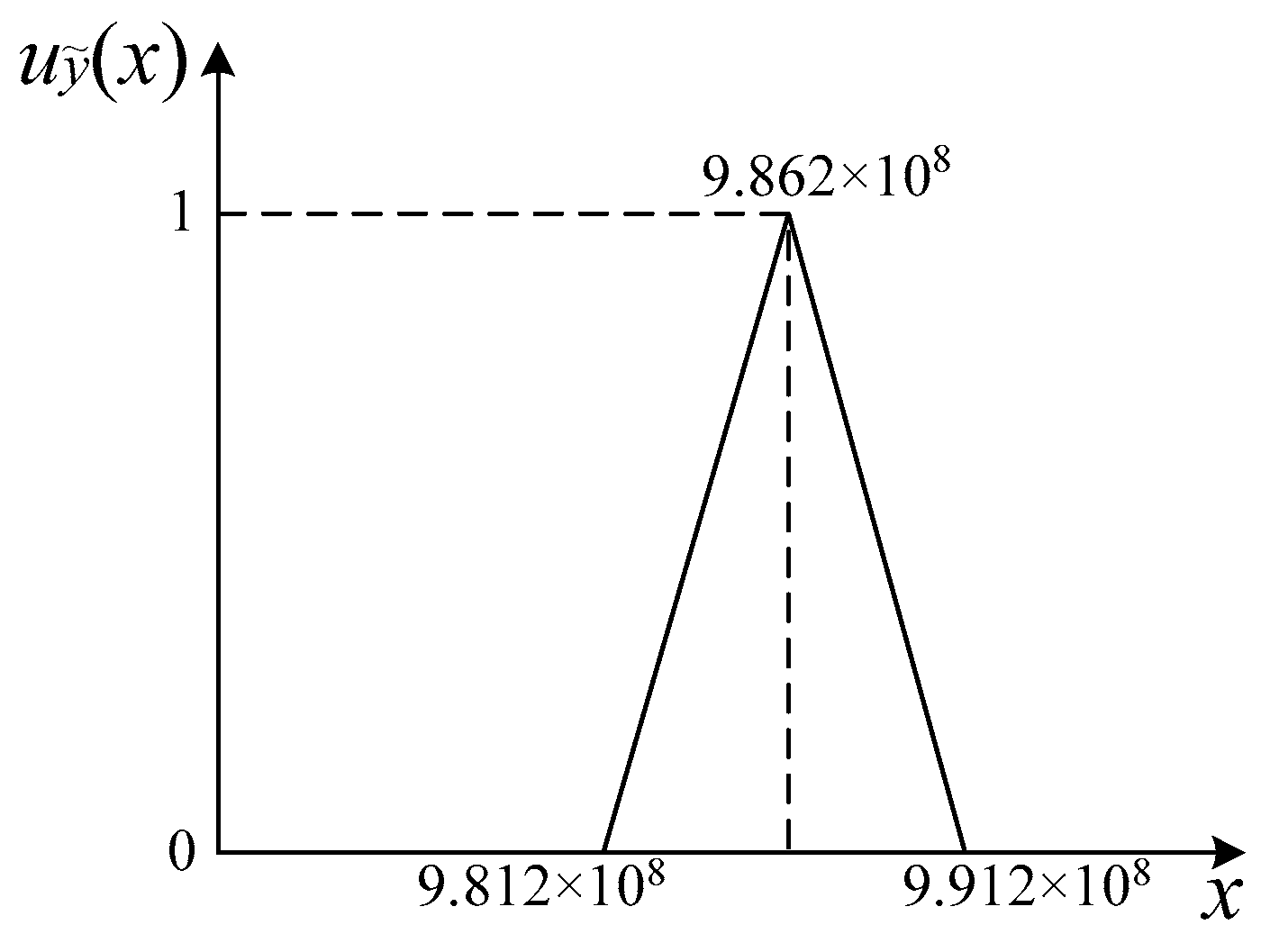
The safety criterion is a typical fuzzy parameter because its allowable values are uncertain in practical engineering. To accomplish the dynamic fuzzy reliability analysis of the turbine blisk with the PDF, the fuzzy safety criterion needs to be transformed into a stochastic safety criterion by the fuzzy entropy principle. When the membership function of fuzzy safety criterion obeys a triangular distribution, the formula and distribution characteristics of the triangular membership function for the turbine blisk are obtained as shown in Equation (20) and Figure 12, respectively.
u y ˜ ( x ) = { x 9.812 × 10 8 5 × 10 6 ,   9.812 × 10 8 < x 9.862 × 10 8 9.912 × 10 8 x 5 × 10 6 ,   9.862 × 10 8 < x 9.912 × 10 8
After confirming the membership function of fuzzy safety criterion, the triangular membership function is transferred into the PDF of safety criterion (namely a stochastic safety criterion) with a normal distribution by the fuzzy entropy theory. The mean value μeq and standard deviation σeq are consequently achieved. The PDF f(zeq) can be expressed by:
f ( z e q ) = 1 2 π × ( 4.980 × 10 6 ) exp ( ( z e q 9.862 × 10 8 ) 2 2 × ( 4.980 × 10 6 ) 2 )
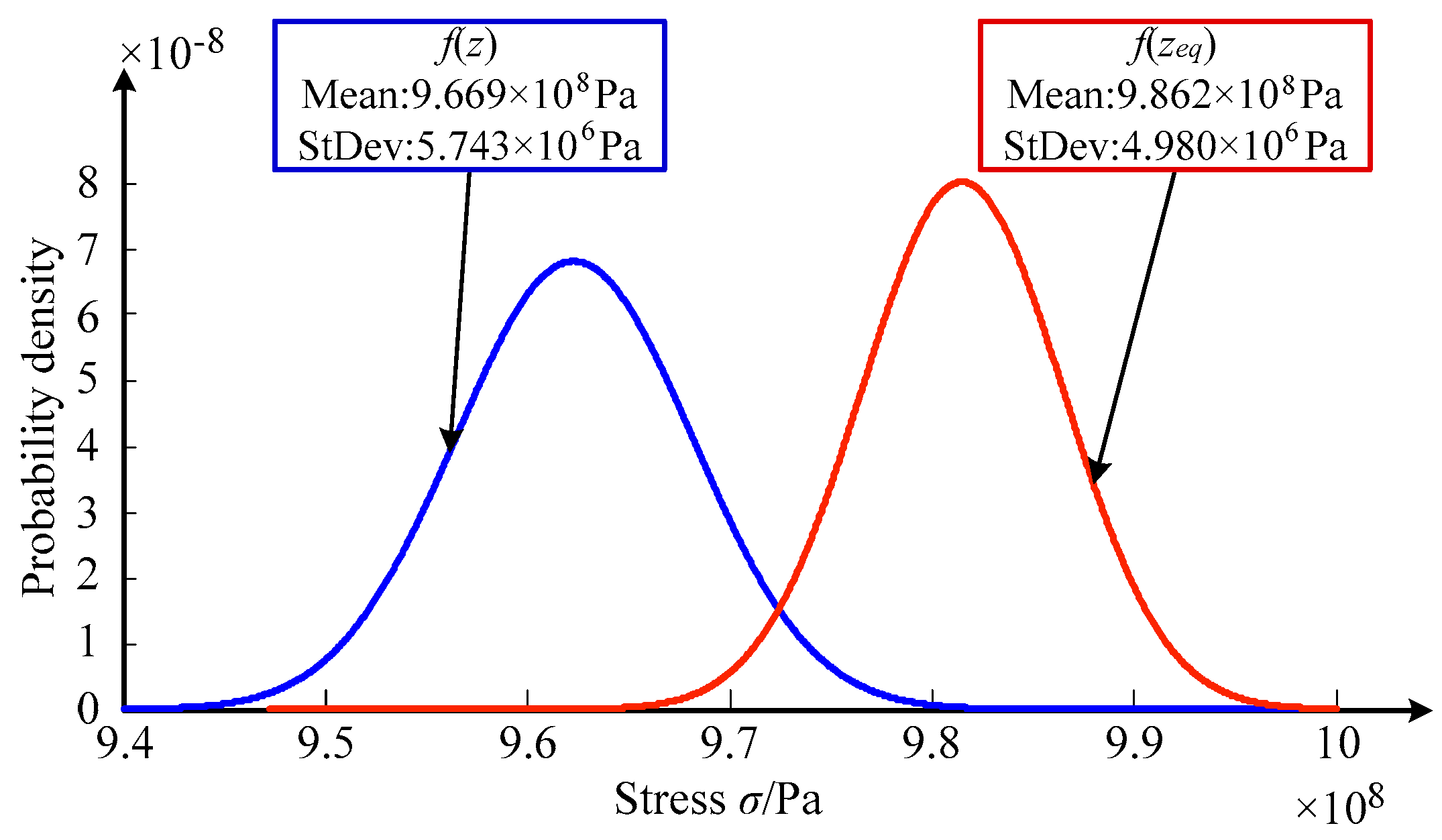
With respect to Equations (19) and (21), the probability density curves f(z) and f(zeq) of stress and the safety criterion of the turbine blisk are drawn in Figure 13, respectively.
As demonstrated in Figure 13, the mean values (9.669 × 10⁸ Pa and 9.862 × 10⁸ Pa) and standard deviations (5.743 × 10⁶ Pa and 4.980 × 10⁶ Pa) of the two methods are acquired. In line with Equation (17), the structural reliability index and reliability degree are β = 2.751 and Pr = 0.9970, respectively.

4. WR-ERSM Verification Procedure

In this section, the proposed WR-ERSM is verified by the comparison with the MC method, ERSM based on least-square and equivalent stochastic transformation method (ESTM).

4.1. Model-Fitting Properties

By the 30 groups of underlined and bold experimental data in Table 2, the model of ERSM is established as:
y ( x ) = 2.015 × 10 8 + 3.734 × 10 6 x 1 + 1.998 × 10 3 x 2 + 9.989 × 10 4 x 3 2.756 × 10 6 x 4 1.137 × 10 4 x 1 2 1.669 × 10 3 x 2 2 + 9.166 × 10 1 x 3 2 + 1.907 × 10 3 x 4 2
In this paper, we adopt the square-error r2 and maximum absolute error rmax to test the fitting accuracy for the WR-ERSM and ERSM. The r2 and rmax are illustrated as follows,
{ r 2 = 1 i = 1 n ( y i y ^ i ) 2 i = 1 n ( y i y ¯ ) 2 r max = max i = 1 n ( | y i y ^ i | S )
in which n is the number of experimental data; yi denotes the authentic output responses; y ^ i is the output responses gained by the mathematical models; y ¯ indicates the mean of the experimental data; S expresses the standard deviation of experimental data. If the square-error r2 is close to 1 and the relative maximum absolute error rmax is close to 0, the fitting accuracy is high.
The remaining 10 groups of the experimental data in Table 2 are employed to test the fitting accuracy of the models (Equations (18) and (22)) with respect to r2 and rmax. The results are listed in Table 3.
As illustrated in Table 3, the proposed WR-ERSM only needs 9 samples for modeling, which is far less than 29 samples for the ERSM. Besides, the fitting time of WR-ERSM is 7.5 hours which is also far less than the 22.39 hours of the ERSM. As for the fitting accuracy, the square-error and maximum absolute error of the WR-ERSM and ERSM are 0.9984, 0.9742 and 0.0535, 0.0834, respectively. Because of the square error 0.9742 < 0.9984→1 and the relative maximum absolute error 0.0834 > 0.0535→0, the fitting accuracy of WR-ERSM is obviously higher than ERSM in modeling precision. Therefore, the WR-ERSM is superior to ERSM in fitting efficiency and accuracy. Because of the high computational accuracy of WR-ERSM, it is also demonstrated to be reasonable and efficient that WR is considered to select better samples to establish ERSM model.

4.2. Simulation Performances for Dynamic Fuzzy Reliability Analysis of Turbine Blisk

In this section, we compare the reliability degree assessments as using four methods, i.e., the MC method, ESTM, ERSM and WR-ERSM. The MC method with direction simulation is considered as the reference when the simulation precisions of other three methods are evaluated. The fuzzy reliability evaluation with the ESTM considers all calculations in the response process in the time domain [0 s, 215 s] without the simplification of the response process just like the ERSM. The ERSM is employed for the dynamic reliability analysis by simplifying the response process as a random parameter without the consideration of both the WR of the output responses in the sample selection for the modeling and the fuzziness of the safety criterion in the reliability analysis. When the WR-ERSM is applied to the dynamic fuzzy reliability estimation of turbine blisk, we completely regard the simplification of the response process, the WR of output responses and the fuzziness of safety criterion. All the calculations and simulation are completed based on the same input variables in Table 1 and computer environment. The computational results are shown in Table 4.
As revealed in Table 4, the WR-ERSM is closer to the MC method than both ESTM and ERSM for the reliability degree of turbine blisk. Besides, the proposed WR-ERSM has higher analytical accuracy than the ERSM and ESTM as the precision 0.9989 for the WR-ERSM is larger than the precision 0.9956 for the ERSM and the precision 0.9981. The result that the precision of the WR-ERSM is superior to the ERSM indicates that considering the fuzziness of the safety criterion besides the WR is efficient for the improvement of structural dynamic reliability analysis. The fact that the precision of the WR-ERSM is superior to the ESTM reveals that the ERSM is effective to deal with the transient in structural dynamic reliability analysis instead of the ESTM. In brief, the WR-ERSM, which considers both the WR of the parameters in the model and the fuzziness of the safety criterion in the analysis, is able to improve the computational accuracy of structural dynamic reliability analysis while keeping to a high degree of reliability. Besides, the structural dynamic fuzzy reliability analysis with the fuzziness of safety criterion is more reasonable and accurate than the structural dynamic reliability analysis without the fuzziness of the safety criterion.
Based on the above results, it is fully demonstrated that the developed WR-ERSM is able to improve computational efficiency and precision for structural dynamic reliability analysis while maintaining a high degree of reliability, by both introducing the WR method to find more effective samples for the ERSM modeling and considering the fuzziness of safety criterion in reliability analysis. The structural dynamic fuzzy reliability analysis with the WR-ERSM is effective and feasible for improving the designs of structures and mechanical system.

5. Conclusions

To improve the computational accuracy and efficiency of structural dynamic fuzzy reliability analysis, we present the weighted regression-based extremum response surface method (WR-ERSM) based on the extremum response surface method (ERSM) and weighted regression (WR), for structural dynamic fuzzy reliability analysis. Through this study, some conclusions are summarized as follows:
(1)
The WR-ERSM is highly precise and efficient in structural dynamic reliability evaluation, since ERSM has the capacity of processing the transient problem;
(2)
The WR approach can improve modeling accuracy so that the proposed WR-ERSM possesses high fitting efficiency and accuracy, due to the requirement of small samples;
(3)
WR-ERSM possesses good simulation performance in structural dynamic fuzzy reliability evaluation, as the fuzzy safety criterion is considered to improve the precision;
(4)
The change rule of turbine blisk structural stress from start to cruise for an aircraft is acquired with the maximum value of structural stress at t = 165 s and the reliability degree (Pr = 0.997) of the turbine blisk.
(5)
The efforts of this study provide a promising method for the dynamic reliability analysis and evaluation of complex structures with respect to the working process.

Author Contributions

Conceptualization, C.-W.F. and Y.-W.F.; Methodology, C.L.; Software, C.L.; Validation, C.L., Y.-W.F. and C.-W.F.; Formal Analysis, C.-W.F.; Investigation, C.L.; Resources, Y.-W.F.; Data Curation, C.-W.F.; Writing-Original Draft Preparation, C.L.; Writing-Review & Editing, C.-W.F.; Visualization, C.L.; Supervision, C.-W.F.; Project Administration, Y.-W.F.; Funding Acquisition, Y.-W.F. and C.-W.F.

Funding

This research was funded by [National Natural Science Foundation of China] grant number [51875465 and 51605016], [Innovation Foundation for Doctor Dissertation of Northwestern Polytechnical University] grant number [CX201932], and [Research Start-up funding of Fudan University] grant number [FDU38341]. The APC was funded by [51875465].

Conflicts of Interest

The authors declare that there is no conflict of interests regarding the publication of this article.

References

  1. Fei, C.W.; Choy, Y.S.; Hu, D.Y.; Bai, G.C.; Tang, W.Z. Dynamic probabilistic design approach of high-pressure turbine blade-tip radial running clearance. Nonlinear Dyn. 2016, 86, 205–223. [Google Scholar] [CrossRef]
  2. Liu, Y.; Meng, L.L.; Liu, K.; Zhang, Y.M. Chatter reliability of milling system based on first-order second-moment method. Int. J. Adv. Manuf. Technol. 2016, 87, 801–809. [Google Scholar] [CrossRef]
  3. Keshtegar, B. Conjugate finite-step length method for efficient and robust structural reliability analysis. Struct. Eng. Mech. 2018, 65, 415–422. [Google Scholar]
  4. Zhang, J.F.; Du, X.P. A second-order reliability method with first-order efficiency. J. Mech. Des. 2010, 132, 101006. [Google Scholar] [CrossRef]
  5. Huang, X.Z.; Li, Y.X.; Zhang, Y.M.; Zhang, X.F. A new direct second-order reliability analysis method. Appl. Math. Model. 2018, 55, 68–80. [Google Scholar] [CrossRef]
  6. Hu, Z.L.; Du, X.P. Efficient reliability-based design with second order approximations. Eng. Optim. 2019, 51, 101–119. [Google Scholar] [CrossRef]
  7. Nakamura, T.; Fujii, K. Probabilistic transient thermal analysis of an atmospheric reentry vehicle structure. Aerosp. Sci. Technol. 2006, 10, 346–354. [Google Scholar] [CrossRef]
  8. Martinez-Velasco, J.A.; Guerra, G. Reliability analysis of distribution systems with photovoltaic generation using a power flow simulator and a parallel Monte Carlo approach. Energies 2016, 9, 537. [Google Scholar] [CrossRef]
  9. Yang, X.J.; Yan, Y.L.; Xu, Z.Q.; Yan, X.Z. FEM simulation on the structural reliability of beam pumping unit based on the methods of Monte-Carlo. Appl. Mech. Mater. 2010, 34–35, 820–824. [Google Scholar] [CrossRef]
  10. Yang, Y.H.; Liu, D.; He, Z.Y.; Luo, Z.J. Optimization of preform shapes by RSM and FEM to improve deformation homogeneity in aerospace forgings. Chin. J. Aeronaut. 2010, 23, 260–267. [Google Scholar]
  11. Allaix, D.L.; Carbone, V.I. An improvement of the response surface method. Struct. Saf. 2011, 32, 165–172. [Google Scholar] [CrossRef]
  12. Kaymaz, I. Application of kriging method to structural reliability problems. Struct. Saf. 2005, 27, 133–151. [Google Scholar] [CrossRef]
  13. Zhao, Z.G.; Duan, X.J.; Wang, Z.M. A novel global method for reliability analysis with kriging. Int. J. Uncertain. Quantif. 2016, 6, 445–466. [Google Scholar] [CrossRef]
  14. Kishore, R.A.; Mahajan, R.L.; Priya, S. Combinatory finite element and artificial neural network model for predicting performance of thermoelectric generator. Energies 2018, 11, 2216. [Google Scholar] [CrossRef]
  15. Gondal, Z.U.R.; Lee, J. Reliability assessment using feed-forward neural network-based approximate meta-models. Proc. Inst. Mech. Eng. Part O J. Risk Reliab. 2012, 226, 448–454. [Google Scholar] [CrossRef]
  16. Rocco, C.M.; Moreno, J.A. Fast Monte Carlo reliability evaluation using support vector machine. Reliab. Eng. Syst. Saf. 2002, 76, 237–243. [Google Scholar] [CrossRef]
  17. Guo, Z.W.; Bai, G.C. Classification using least squares support vector machine for reliability analysis. Appl. Math. Mech. 2009, 30, 853–864. [Google Scholar] [CrossRef]
  18. Zhang, C.Y.; Bai, G.C. Extremum response surface method of reliability analysis on two-link flexible rotor manipulator. J. Cent. South Univ. 2012, 19, 101–107. [Google Scholar] [CrossRef]
  19. Fei, C.W.; Tang, W.Z.; Bai, G.C. Nonlinear dynamic probabilistic design of turbine disk-radial deformation using extremum response surface method-based support vector machine of regression. Proc. Inst. Mech. Eng. Part G J. Aerosp. Eng. 2015, 229, 290–300. [Google Scholar] [CrossRef]
  20. Fei, C.W.; Tang, W.Z.; Bai, G.C. Dynamic probabilistic design for blade deformation with SVM-ERSM. Aircr. Eng. Aerosp. Technol. 2015, 87, 312–321. [Google Scholar] [CrossRef]
  21. Broadie, M.; Du, Y. Risk estimation via weighted regression. In Proceedings of the 2011 Winter Simulation Conference, Phoenix, AZ, USA, 11–14 December 2011; pp. 3859–3870. [Google Scholar]
  22. Kaymaz, I.; McMahon, C.A. A response surface method based on weighted regression for structural reliability analysis. Probabilistic Eng. Mech. 2005, 20, 11–17. [Google Scholar] [CrossRef]
  23. Guo, S.X.; Lu, Z.Z. Procedure for computing the possibility and fuzzy probability of failure of structures. Appl. Math. Mech. 2003, 24, 338–343. [Google Scholar]
  24. Hurtado, J.E.; Alvarez, D.A.; Ramirez, J. Fuzzy structural analysis based on fundamental reliability concepts. Comput. Struct. 2012, 112, 183–192. [Google Scholar] [CrossRef]
  25. Zhu, S.P.; Liu, Q.; Zhou, J.; Yu, Z.Y. Fatigue reliability assessment of turbine discs under multi-source uncertainties. Fatigue Fract. Eng. Mater. Struct. 2018, 41, 1291–1305. [Google Scholar] [CrossRef]
  26. Huang, H.Z. Structural reliability analysis using fuzzy sets theory. Eksploat. I Niezawodn. Maint. Reliab. 2012, 4, 284–294. [Google Scholar]
  27. Wang, Z.L.; Li, Y.F.; Huang, H.Z.; Liu, Y. Reliability analysis of structure for fuzzy safety state. Intell. Autom. Soft Comput. 2012, 18, 215–224. [Google Scholar] [CrossRef]
  28. Zhang, M.; Lu, S. A reliability model of blade to avoid resonance considering multiple fuzziness. Proc. Inst. Mech. Eng. Part O J. Risk Reliab. 2014, 228, 641–652. [Google Scholar] [CrossRef]
  29. Zhu, S.P.; Liu, Q.; Peng, W.; Zhang, X.C. Computational-experimental approaches for fatigue reliability assessment of turbine bladed disks. Int. J. Mech. Sci. 2018, 142–143, 502–517. [Google Scholar] [CrossRef]
  30. Lee, S.H.; Kwak, B.M. Response surface augmented moment method for efficient reliability analysis. Struct. Saf. 2006, 28, 261–272. [Google Scholar] [CrossRef]
  31. Afsan, B.M.U.; Basu, C.K. Fuzzy topological entropy of fuzzy continuous functions on fuzzy topological spaces. Appl. Math. Lett. 2011, 24, 2030–2033. [Google Scholar] [CrossRef] [Green Version]
  32. Markechova, D.; Riecan, B. Entropy of fuzzy partitions and entropy of fuzzy dynamical systems. Entropy 2016, 18, 19. [Google Scholar] [CrossRef]
  33. Fei, C.W.; Tang, W.Z.; Bai, G.C. Novel method and model for dynamic reliability optimal design of turbine blade deformation. Aerosp. Sci. Technol. 2014, 39, 588–595. [Google Scholar] [CrossRef]
  34. Zhang, C.Y.; Lu, C.; Fei, C.W.; Liu, L.J.; Choy, Y.Z.; Su, X.G. Multiobject reliability analysis of turbine blisk with multidiscipline under multiphysical field interaction. Adv. Mater. Sci. Eng. 2015, 2015, 649046. [Google Scholar] [CrossRef]
  35. Li, L.Y.; Lu, Z.Z. Importance analysis for model with mixed uncertainties. Fuzzy Sets Syst. 2017, 310, 90–107. [Google Scholar] [CrossRef]
  36. Sun, J.; Luo, Y. Reliability-optimization design based on fuzzy entropy for cylinder head bolts. J. Appl. Sci. 2013, 13, 5198–5203. [Google Scholar] [CrossRef]
  37. Lattime, S.B.; Steinetz, B.M. Turbine engine clearance control systems: Current practices and future directions. J. Propuls. Power 2004, 20, 302–311. [Google Scholar] [CrossRef]
  38. Fei, C.W.; Choy, Y.S.; Hu, D.Y.; Bai, G.C.; Tang, W.Z. Transient probabilistic analysis for turbine blade-tip radial clearance with multiple components and multi-physics fields based on DCERSM. Aerosp. Sci. Technol. 2016, 50, 62–70. [Google Scholar] [CrossRef]
  39. Wang, H.B.; Wang, Z.G.; Sun, M.B.; Qin, N. Large eddy simulation of a hydrogen-fueled scramjet combustor with dual cavity. Acta Astronaut. 2015, 108, 119–128. [Google Scholar] [CrossRef]
  40. Lu, C.; Feng, Y.W.; Fei, C.W.; Xue, X.F. Probabilistic analysis method of turbine blisk with multi-failure modes by two-way fluid-thermal-solid coupling. Proc. Inst. Mech. Eng. Part C J. Mech. Eng. Sci. 2018, 232, 2873–2886. [Google Scholar] [CrossRef]
  41. Liu, J.; Nan, Z.; Yi, P. Validation and application of three-dimensional discontinuous deformation analysis with tetrahedron finite element meshed block. Acta Mech. Sin. 2012, 28, 1602–1616. [Google Scholar] [CrossRef]
  42. Fei, C.W.; Bai, G.C. Extremum selection method of random variables for nonlinear dynamic reliability analysis of turbine blade deformation. Propuls. Power Res. 2012, 1, 58–63. [Google Scholar] [CrossRef]
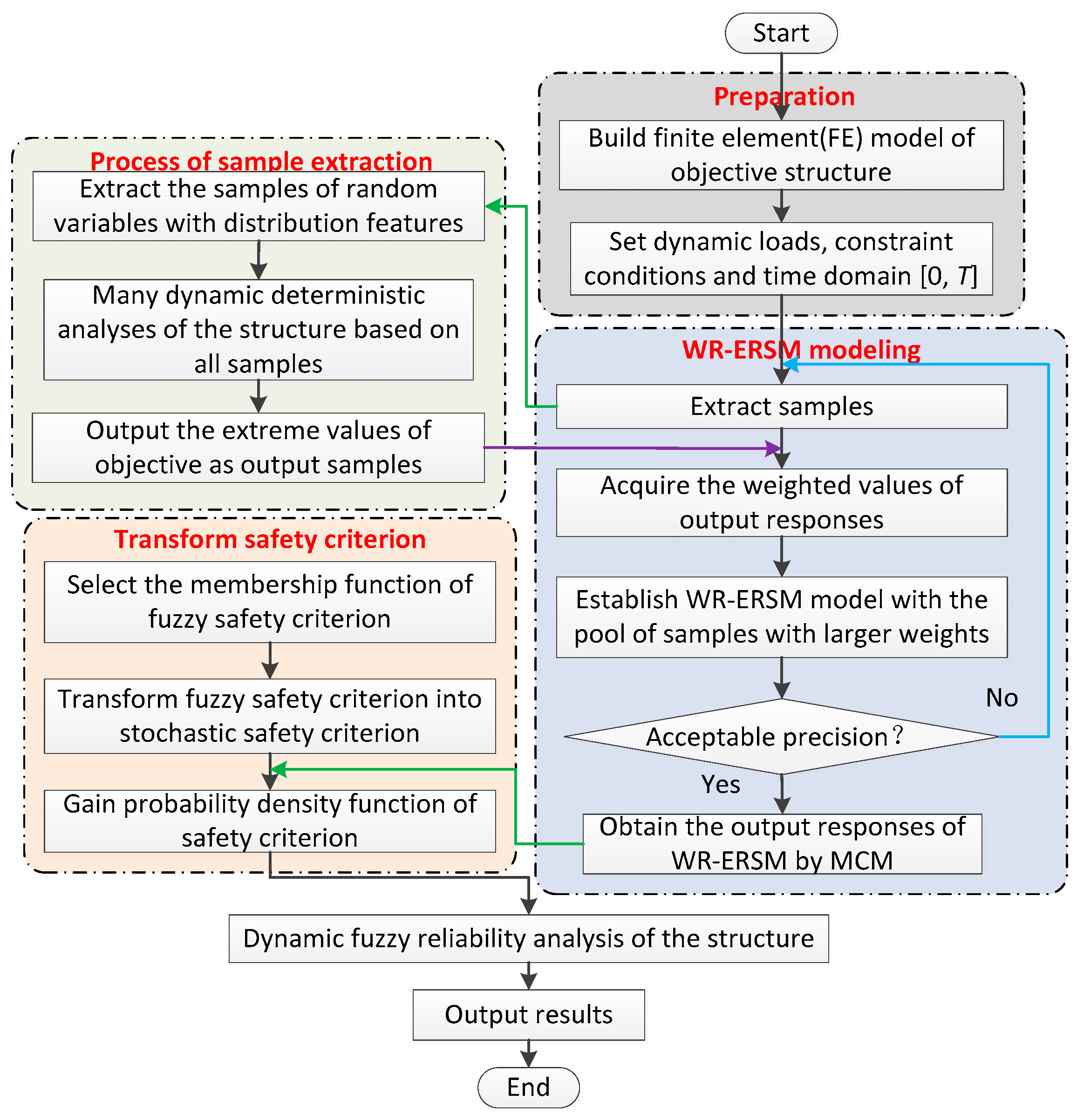
Figure 1. Flow chart of structural dynamic fuzzy reliability analysis with weighted regression extremum response surface method (WR-ERSM).
Energies 12 01588 g001
Figure 2. Basic thoughts of ERSM and WR-ERSM.
Energies 12 01588 g002
Figure 3. Change curve of angular speed in time domain [0 s, 215 s].
Energies 12 01588 g003
Figure 4. Geometric model of turbine blisk.
Energies 12 01588 g004
Figure 5. Finite element (FE) model of turbine blisk.
Energies 12 01588 g005
Figure 6. FE model of flow field.
Energies 12 01588 g006
Figure 7. Stress variation curve of turbine blisk during [0 s, 215 s].
Energies 12 01588 g007
Figure 8. Pressure distribution on fluid–structure coupling interface.
Energies 12 01588 g008
Figure 9. Stress distribution on turbine blisk.
Energies 12 01588 g009
Figure 10. The simulation history of turbine blisk stress.
Energies 12 01588 g010
Figure 11. The histogram of turbine blisk stress.
Energies 12 01588 g011
Figure 12. The triangular membership function of the turbine blisk.
Energies 12 01588 g012
Figure 13. Distribution features of structural stress and safety criterion.
Energies 12 01588 g013
Table 1. The statistical characteristics of random input variables.
ParametersVariableDistributionMean, μSt.Dev., δ
Inlet velocity (m·s−1)vNormal1685.04
Inlet pressure (Pa)PNormal600,00012,000
Material density (kg·m−3)ρNormal8210246
Angular speed (rad·s−1)wNormal116835
Table 2. Weighted samples based on weighted regression analysis.
Parameters and Weighted CoefficientParameters and Weighted Coefficient
v m·s−1P, ×105 Paρ kg·m−3w rad·s−1σ × 108 PaWv, m·s−1P, ×105 Paρ, kg·m−3w, rad·s−1σ, ×108 PaW
168.006.00821011689.6870.9105173.046.00821011339.0980.9694
162.966.00821011689.6930.9099168.006.12821011339.1050.9687
168.005.88821011689.6860.9106168.006.00796411338.8270.9992
168.006.00796411689.3920.9391173.045.88796411689.3850.9398
168.006.00821011339.1050.9687173.045.88821011339.0980.9694
173.046.00821011689.6860.9391162.966.12796411689.3980.9385
168.006.12821011689.6870.9105162.966.12821011339.1110.9681
168.006.128210120310.290.8576168.006.008456120310.590.8575
162.965.88821011689.6870.9105168.006.12796411338.8290.9989
162.966.00796411689.3910.9392162.966.00845611339.3890.9394
162.966.00821011339.1050.9687168.005.88845611339.3830.9400
168.005.88796411689.3910.9392173.046.12796411689.3850.9398
168.005.88821011339.1050.9687173.046.12821011339.0980.9694
168.006.00796411338.8270.9992173.046.00845611339.3760.9407
173.046.12821011689.6870.9105168.006.12845611339.3830.9400
162.966.12821011689.6930.9099162.965.88796411689.3980.9385
168.006.008210120310.280.8576173.046.008210120310.280.8576
173.045.88821011689.6810.9111162.965.88821011339.1110.9681
173.046.00796411689.3850.9398162.966.00796411338.8270.9992
168.006.12796411689.3910.9392168.005.88796411338.8260.9993
Note: the symbols v, P, ρ and w are the inlet velocity, inlet pressure, material density and angular speed, respectively; σ presents the turbine blisk stress; W denotes the weighted value. Additionally, the underlined samples (20 samples) are used to establish the WR-ERSM model, and the underlined and bold samples (30 samples) are applied to derive the ERSM model.
Table 3. The computational results of the ERSM model and WR-ERSM model.
MethodFitting ERSM ModelFitting Accuracy
Sample NumberFitting Time, hr2rmax
WR-ERSM97.050.99840.0535
ERSM2922.390.97420.0834
Table 4. The simulation results of turbine blisk dynamic reliability analyses with four methods.
MethodsPrErrorsPrecision, %
MC method0.9981--
ESTM0.99620.001999.81
ERSM0.99370.004499.56
WR-ERSM0.99700.001199.89