Concatenate Convolutional Neural Networks for Non-Intrusive Load Monitoring across Complex Background


Abstract
:1. Introduction
2. Related Work
3. Concatenate Convolutional Neural Networks
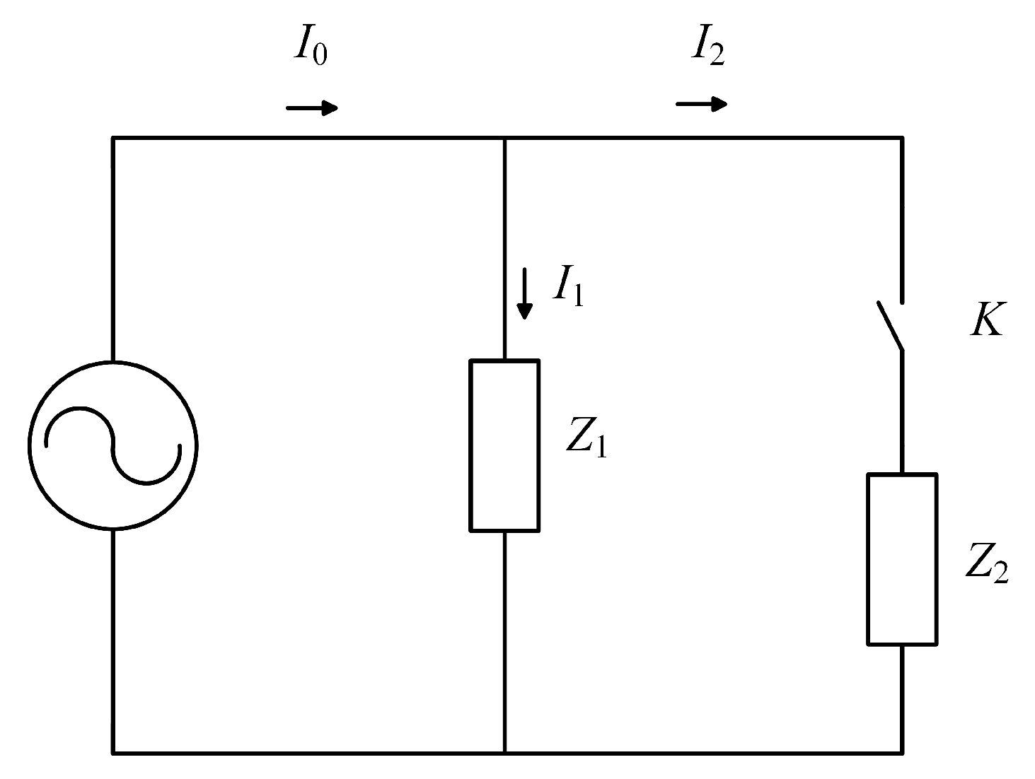
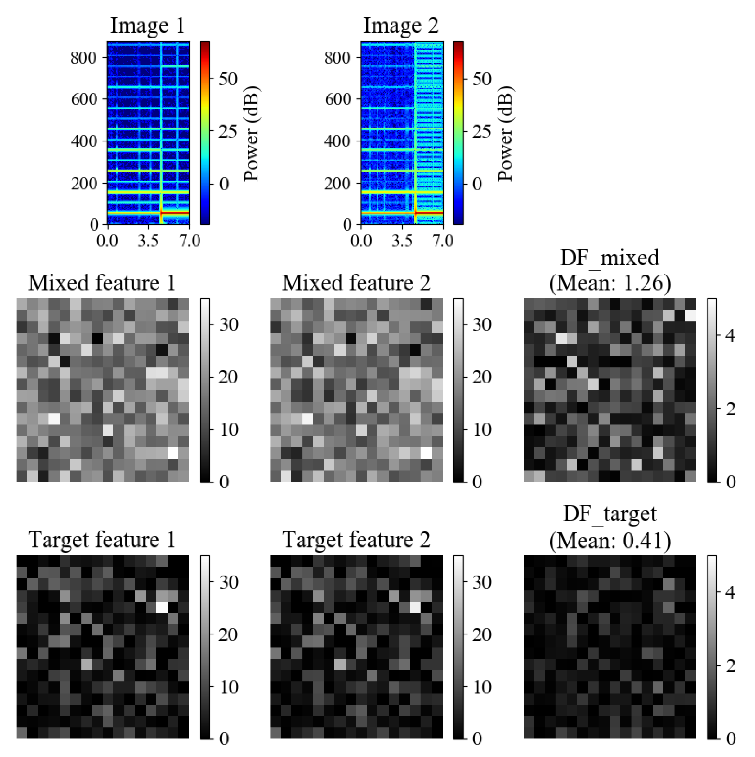
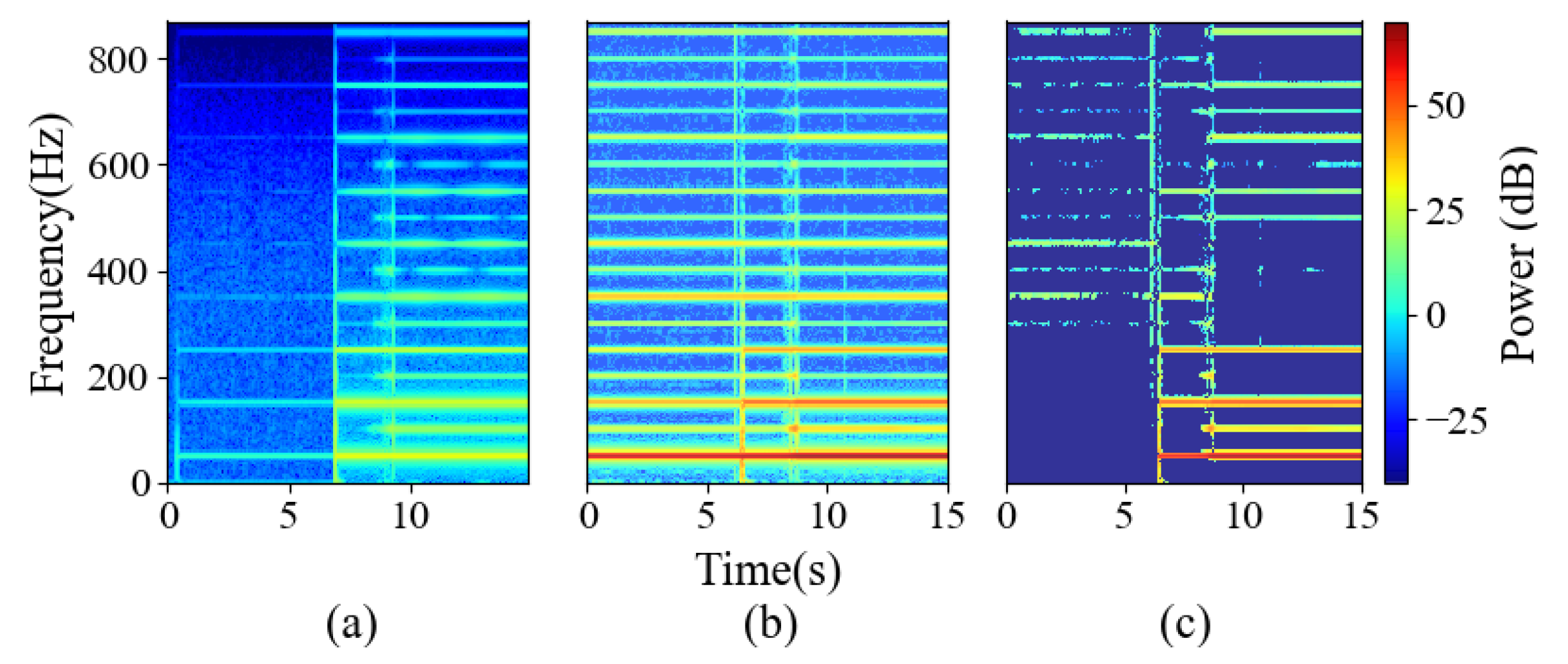
3.1. Problem Statement
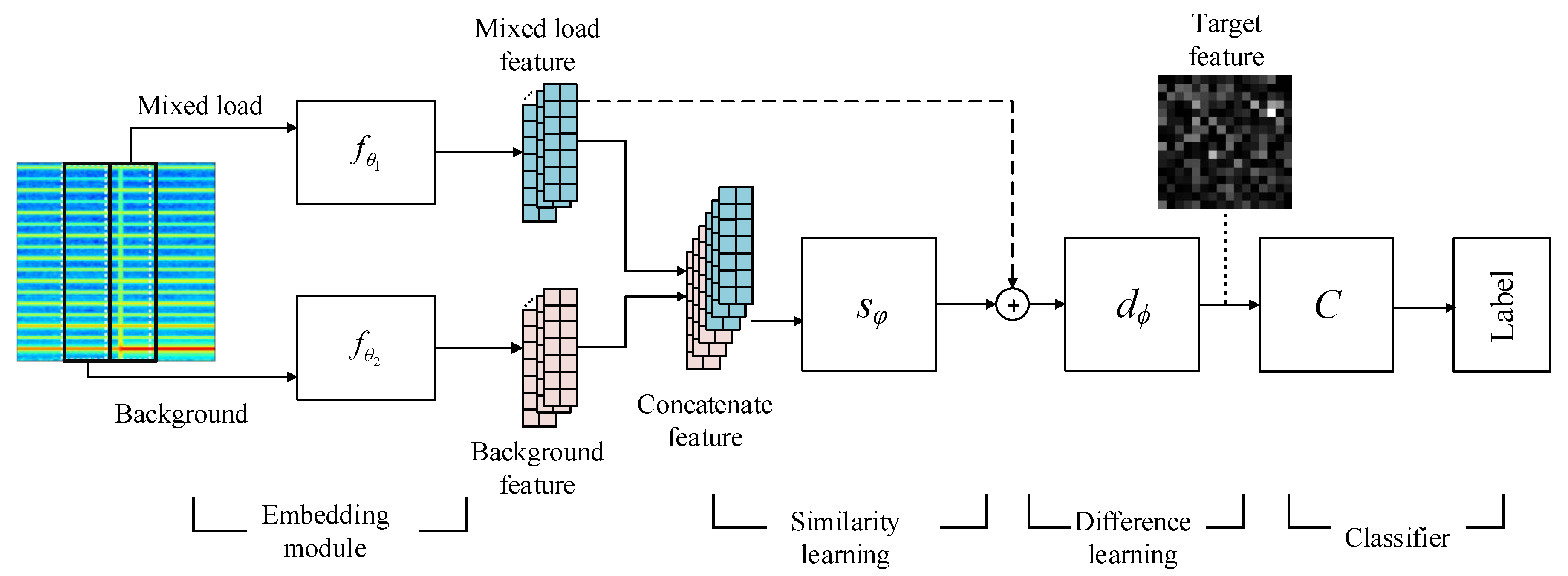
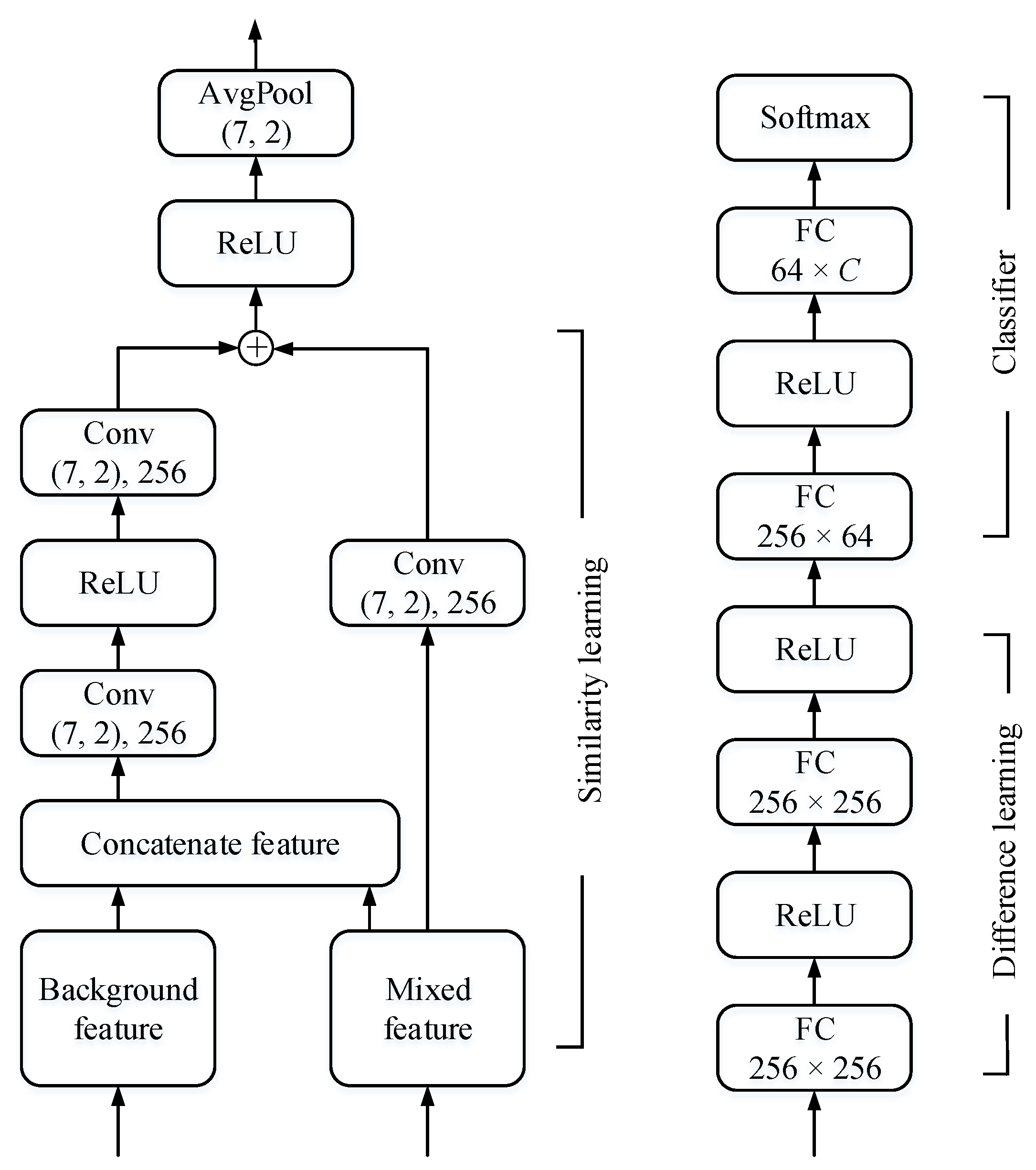
3.2. Model Architecture
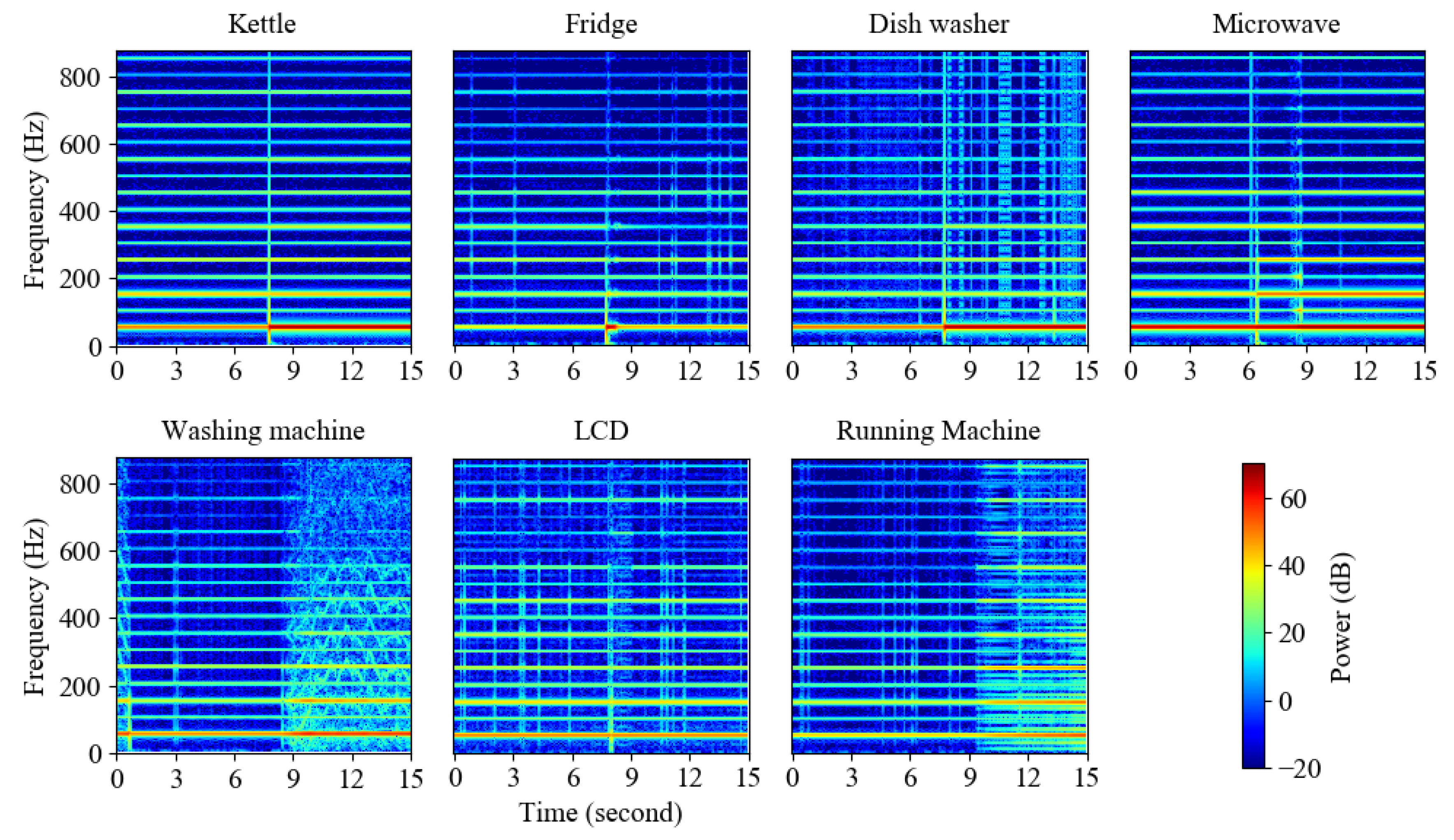
4. Experiments and Discussion
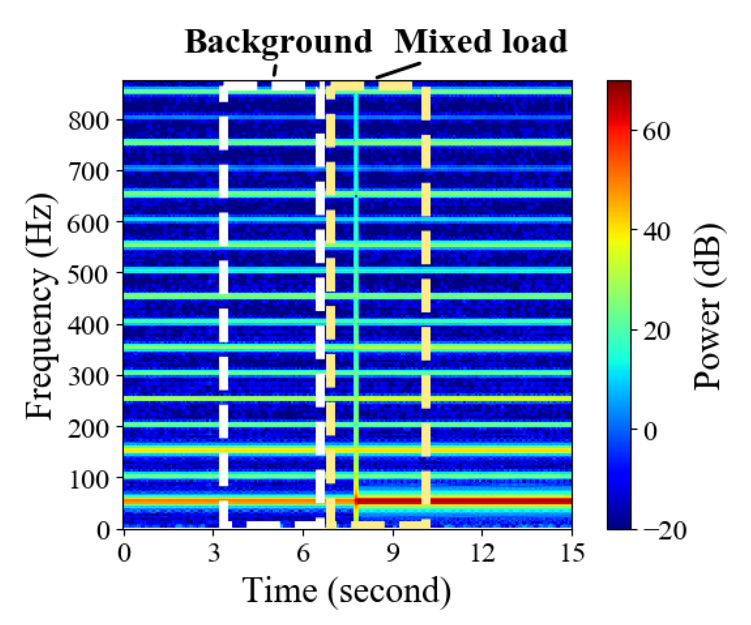
4.1. Dataset and Data Preprocessing
4.1.1. UK-DALE
4.1.2. BLUED
4.2. Experimental Infrastructure
4.3. The Recognition Result on UK-DALE
4.4. The Recognition Result on BLUED
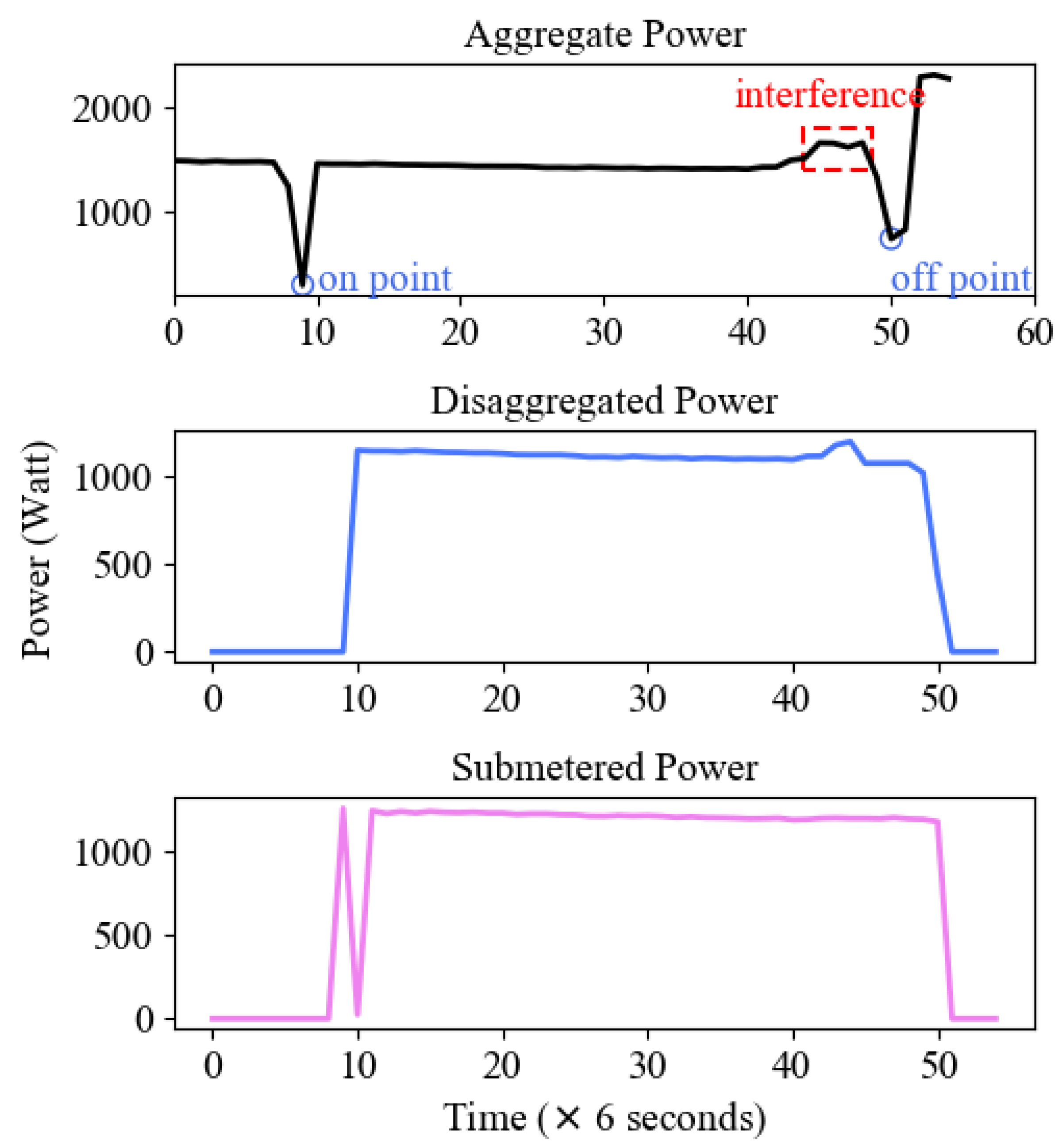
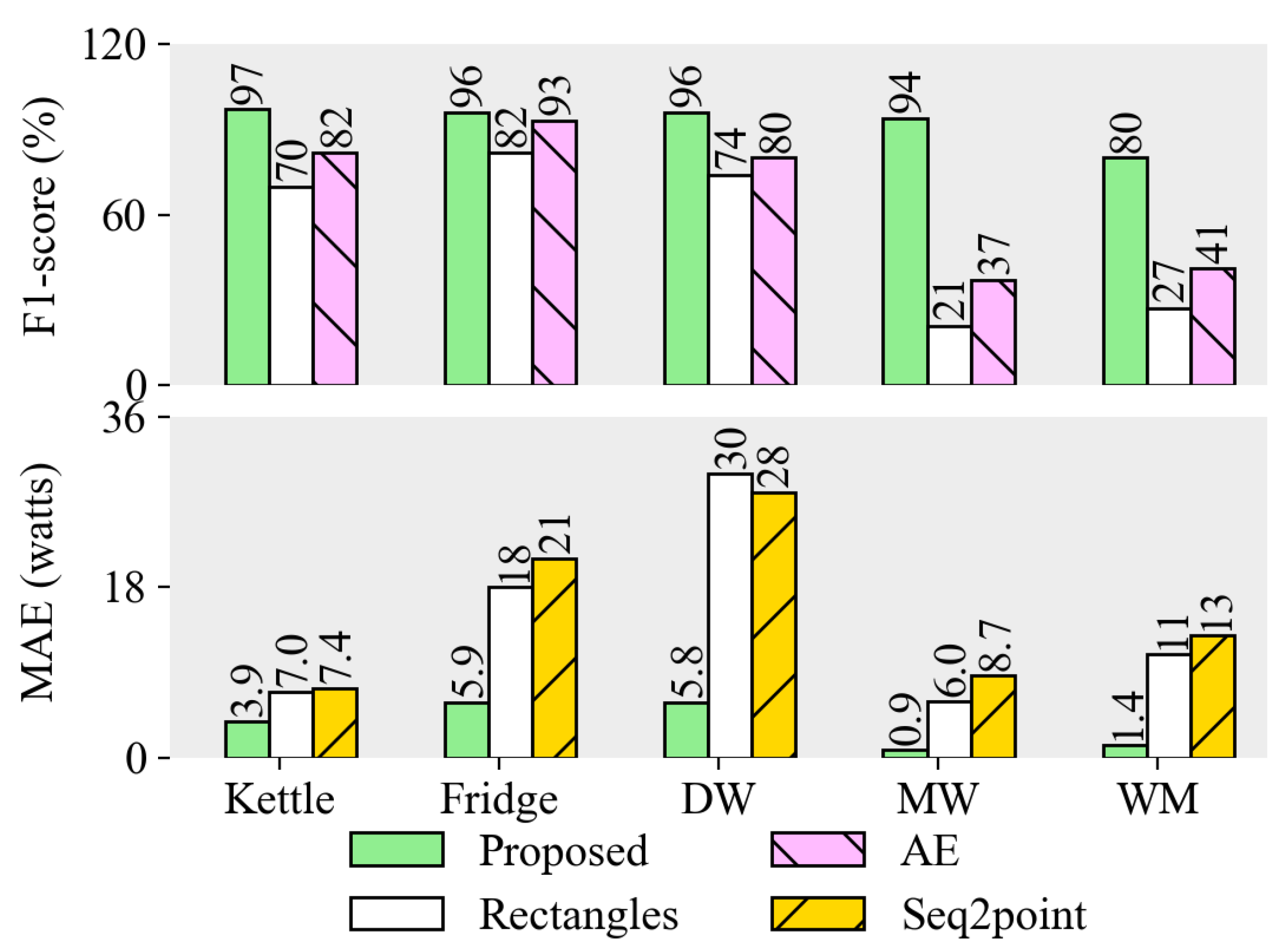
4.5. The Energy Disaggregation Result on UK-DALE
| Algorithm 1 Work Flow of Energy Disaggregation |
| Require: The aggregate power data at time t, The on-events recognized by the classification task, The power of individual appliance l,
|
5. Conclusions
Author Contributions
Funding
Conflicts of Interest
References
- Wytock, M.; Kolter, J.Z. Contextually Supervised Source Separation with Application to Energy Disaggregation. In Proceedings of the 28th AAAI Conference on Artificial Intelligence, Québec City, QC, Canada, 27–31 July 2014; pp. 486–492. [Google Scholar]
- Yu, L.; Li, H.; Feng, X.; Duan, J. Nonintrusive appliance load monitoring for smart homes: Recent advances and future issues. IEEE Instrum. Meas. Mag. 2016, 19, 56–62. [Google Scholar] [CrossRef]
- Siano, P. Demand response and smart grids—A survey. Renew. Sustain. Energy Rev. 2014, 30, 461–478. [Google Scholar] [CrossRef]
- Ephrat, A.; Mosseri, I.; Lang, O.; Dekel, T.; Wilson, K.; Hassidim, A.; Freeman, W.T.; Rubinstein, M. Looking to listen at the cocktail party: A speaker-independent audio-visual model for speech separation. ACM Trans. Graph. 2018, 37, 112. [Google Scholar] [CrossRef]
- Mogami, S.; Sumino, H.; Kitamura, D.; Takamune, N.; Takamichi, S.; Saruwatari, H.; Ono, N. Independent Deeply Learned Matrix Analysis for Multichannel Audio Source Separation. In Proceedings of the IEEE 26th European Signal Processing Conference (EUSIPCO), Rome, Italy, 3–7 September 2018; pp. 1557–1561. [Google Scholar]
- Chollet, F. Xception: Deep learning with depthwise separable convolutions. In Proceedings of the IEEE Conference on Computer Vision and Pattern Recognition (CVPR), Honolulu, HA, USA, 22–25 July 2017; pp. 1251–1258. [Google Scholar]
- He, K.; Zhang, X.; Ren, S.; Sun, J. Deep residual learning for image recognition. In Proceedings of the IEEE Conference on Computer Vision and Pattern Recognition (CVPR), Las Vegas, NV, USA, 27–30 June 2016; pp. 770–778. [Google Scholar]
- Huang, G.; Liu, Z.; Van Der Maaten, L.; Weinberger, K.Q. Densely connected convolutional networks. In Proceedings of the IEEE Conference on Computer Vision and Pattern Recognition (CVPR), Honolulu, HA, USA, 22–25 July 2017; pp. 2261–2269. [Google Scholar]
- Kelly, J.; Knottenbelt, W. The UK-DALE dataset domestic appliance-level electricity demand and whole-house demand from five UK homes. Sci. Data 2015, 2, 150007. [Google Scholar] [CrossRef] [PubMed]
- Anderson, K.; Ocneanu, A.; Benitez, D.; Carlson, D.; Rowe, A.; Berges, M. BLUED: A fully labeled public dataset for event-based non-intrusive load monitoring research. In Proceedings of the 2nd KDD Workshop on Data Mining Applications in Sustainability (SustKDD), Beijing, China, 12–16 August 2012; pp. 12–16. [Google Scholar]
- Hart, G.W. Nonintrusive appliance load monitoring. Proc. IEEE 1992, 80, 1870–1891. [Google Scholar] [CrossRef]
- Carli, R.; Dotoli, M. Energy scheduling of a smart home under nonlinear pricing. In Proceedings of the 53rd IEEE Conference on Decision and Control, Los Angeles, CA, USA, 15–17 December 2014; pp. 5648–5653. [Google Scholar]
- Sperstad, I.B.; Korpås, M. Energy Storage Scheduling in Distribution Systems Considering Wind and Photovoltaic Generation Uncertainties. Energies 2019, 12, 1231. [Google Scholar] [CrossRef]
- Hosseini, S.M.; Carli, R.; Dotoli, M. Model Predictive Control for Real-Time Residential Energy Scheduling under Uncertainties. In Proceedings of the 2018 IEEE International Conference on Systems, Man, and Cybernetics (SMC), Miyazaki, Japan, 7–10 October 2018; pp. 1386–1391. [Google Scholar]
- Kelly, J.; Knottenbelt, W. Neural NILM: Deep neural networks applied to energy disaggregation. In Proceedings of the 2nd ACM International Conference on Embedded Systems for Energy-Efficient Built Environments, Seoul, South Korea, 4–5 November 2015; pp. 55–64. [Google Scholar]
- Parson, O.; Ghosh, S.; Weal, M.; Rogers, A. Non-intrusive load monitoring using prior models of general appliance types. In Proceedings of the 26th AAAI Conference on Artificial Intelligence, Toronto, ON, Canada, 22–26 July 2012; pp. 356–362. [Google Scholar]
- Chang, H.H.; Chen, K.L.; Tsai, Y.P.; Lee, W.J. A new measurement method for power signatures of nonintrusive demand monitoring and load identification. IEEE Trans. Ind. Appl. 2012, 48, 764–771. [Google Scholar] [CrossRef]
- Froehlich, J.; Larson, E.; Gupta, S.; Cohn, G.; Reynolds, M.; Patel, S. Disaggregated end-use energy sensing for the smart grid. IEEE Pervasive Comput. 2011, 10, 28–39. [Google Scholar] [CrossRef]
- Kahl, M.; Haq, A.U.; Kriechbaumer, T.; Jacobsen, H.A. WHITED—A Worldwide Household and Industry Transient Energy Data Set. In Proceedings of the 3rd International Workshop on Non-Intrusive Load Monitoring, Vancouver, BC, Canada, 14–15 May 2016. [Google Scholar]
- Chui, K.; Lytras, M.; Visvizi, A. Energy Sustainability in Smart Cities: Artificial intelligence, smart monitoring, and optimization of energy consumption. Energies 2018, 11, 2869. [Google Scholar] [CrossRef]
- Figueiredo, M.; De Almeida, A.; Ribeiro, B. Home electrical signal disaggregation for non-intrusive load monitoring (NILM) systems. Neurocomputing 2012, 96, 66–73. [Google Scholar] [CrossRef]
- Le, T.T.H.; Kim, H. Non-Intrusive Load Monitoring Based on Novel Transient Signal in Household Appliances with Low Sampling Rate. Energies 2018, 11, 3409. [Google Scholar] [CrossRef]
- Gillis, J.M.; Morsi, W.G. Non-intrusive load monitoring using semi supervised machine learning and wavelet design. IEEE Trans. Smart Grid 2016, 8, 2648–2655. [Google Scholar] [CrossRef]
- Hassan, T.; Javed, F.; Arshad, N. An empirical investigation of V-I trajectory based load signatures for non-intrusive load monitoring. IEEE Trans. Smart Grid 2014, 5, 870–878. [Google Scholar] [CrossRef]
- He, K.; Stankovic, L.; Liao, J.; Stankovic, V. Non-intrusive load disaggregation using graph signal processing. IEEE Trans. Smart Grid 2018, 9, 1739–1747. [Google Scholar] [CrossRef]
- Makonin, S.; Popowich, F.; Bajić, I.V.; Gill, B.; Bartram, L. Exploiting HMM sparsity to perform online real-time nonintrusive load monitoring. IEEE Trans. Smart Grid 2016, 7, 2575–2585. [Google Scholar] [CrossRef]
- Cominola, A.; Giuliani, M.; Piga, D.; Castelletti, A.; Rizzoli, A.E. A hybrid signature-based iterative disaggregation algorithm for non-intrusive load monitoring. Appl. Energy 2017, 185, 331–344. [Google Scholar] [CrossRef]
- Barsim, K.S.; Yang, B. On the Feasibility of Generic Deep Disaggregation for Single-Load Extraction. In Proceedings of the 4th International Workshop on Non-Intrusive Load Monitoring, Austin, TX, USA, 7–8 March 2018; pp. 1–5. [Google Scholar]
- Zhang, C.; Zhong, M.; Wang, Z.; Goddard, N.; Sutton, C. Sequence-to-point learning with neural networks for non-intrusive load monitoring. In Proceedings of the 32nd AAAI Conference on Artificial Intelligence, New Orleans, LA, USA, 2–7 February 2018; pp. 2604–2611. [Google Scholar]
- Mocanu, E.; Nguyen, P.H.; Gibescu, M. Energy disaggregation for real-time building flexibility detection. In Proceedings of the 2016 IEEE Power and Energy Society General Meeting (PESGM), Boston, MA, USA, 17–21 July 2016; pp. 1–5. [Google Scholar]
- Hanzo, L.; Yang, L.L.; Kuan, E.L.; Yen, K. Single and Multi-Carrier DS-CDMA: Multi-User Detection Space-Time Spreading Synchronisation Networking and Standards; John Wiley & Sons: New York, NY, USA, 2003; pp. 35–80. [Google Scholar]
- Patri, O.P.; Panangadan, A.V.; Chelmis, C.; Prasanna, V.K. Extracting discriminative features for event-based electricity disaggregation. In Proceedings of the 2014 IEEE Conference on Technologies for Sustainability (SusTech), Ogden, UT, USA, 30 July 2014; pp. 232–238. [Google Scholar]
- Kinga, D.P.; Ba, J. Adam: A Method for Stochastic Optimization. In Proceedings of the 3rd International Conference for Learning Representations (ICLR), San Diego, CA, USA, 7–9 May 2015. [Google Scholar]
- Makonin, S.; Popowich, F. Efficient sparse matrix processing for nonintrusive load monitoring (NILM). Energy Efficien. 2014, 8, 809–814. [Google Scholar] [CrossRef]


| Appliance | House 1 | House 2 | House 5 |
|---|---|---|---|
| Kettle | 4430 | 508 | 171 |
| Fridge | 7525 | 2172 | 2453 |
| DW | 2797 | 163 | 235 |
| MW | 536 | 299 | 29 |
| WM | 12311 | 785 | 521 |
| LCD | 4022 | 862 | 387 |
| Appliance | Label | #Events |
|---|---|---|
| Fridge | Phase A, 1 | 282 |
| Lights1 (backyard lights, washroom light, bedroom lights) | Phase A, 2 | 17 |
| High-Power1 (Hair dryer, air compressor, kitchen aid chopper) | Phase A, 3 | 18 |
| Lights2 (desktop lamp, basement light, closet lights) | Phase B, 1 | 38 |
| High-Power2 (printer, iron, garage door) | Phase B, 2 | 52 |
| Computer and monitor (computer, LCD monitor, DVR) | Phase B, 3 | 130 |
| Model | Model Input | Model Description |
|---|---|---|
| CNN (baseline 1) | One original spectrogram | CNN with a FC classifier |
| CNN-SE (baseline 2) | One original spectrogram subtracts the estimated background | CNN with a FC classifier |
| Concatenate-CNN | Two spectrograms split from the original spectrograms | CNN with a similarity learning module, a difference learning module and a FC classifier |
| Model | Metrics | Kettle | Fridge | DW | MW | WM | LCD | RM | Average |
|---|---|---|---|---|---|---|---|---|---|
| Xception | Recall | 91.3 | 98.1 | 79.1 | 98.7 | 96.9 | 63.5 | 42.9 | 81.5 |
| Precision | 91.7 | 99.9 | 39.1 | 98.3 | 77.6 | 99.5 | 81.8 | 84.0 | |
| F1-score | 91.5 | 99.0 | 52.3 | 98.5 | 86.2 | 77.5 | 56.3 | 80.2 | |
| Xception-SE | Recall | 97.6 | 93.9 | 77.3 | 98.7 | 96.3 | 87.6 | 33.3 | 83.5 |
| Precision | 93.0 | 99.0 | 35.9 | 98.7 | 95.6 | 98.3 | 87.5 | 86.8 | |
| F1-score | 95.3 | 96.4 | 49.0 | 98.7 | 95.9 | 92.6 | 48.3 | 82.3 | |
| Concatenate-Xception | Recall | 99.6 | 99.6 | 84.7 | 96.7 | 98.9 | 71.9 | 52.4 | 86.2 |
| Precision | 95.3 | 99.5 | 40.7 | 99.7 | 93.0 | 98.4 | 91.7 | 88.3 | |
| F1-score | 97.4 | 99.6 | 55.0 | 98.1 | 95.9 | 83.1 | 66.7 | 85.1 | |
| DenseNet-121 | Recall | 100 | 99.8 | 71.8 | 99.7 | 95.5 | 81.2 | 71.4 | 88.5 |
| Precision | 91.4 | 99.6 | 66.9 | 98.7 | 85.7 | 99.4 | 71.4 | 87.6 | |
| F1-score | 95.5 | 99.7 | 69.2 | 99.2 | 90.3 | 89.4 | 71.4 | 87.8 | |
| DenseNet-121-SE | Recall | 99.2 | 86.4 | 87.7 | 99.0 | 97.8 | 74.2 | 71.4 | 88.0 |
| Precision | 95.6 | 99.9 | 22.3 | 99.7 | 95.5 | 99.5 | 78.9 | 84.5 | |
| F1-score | 97.4 | 92.7 | 35.6 | 99.3 | 96.7 | 85.0 | 75.0 | 83.1 | |
| Concatenate-DenseNet-121 | Recall | 100 | 99.6 | 77.9 | 99.3 | 92.4 | 93.0 | 57.1 | 88.5 |
| Precision | 92.5 | 99.2 | 62.6 | 100 | 95.9 | 98.9 | 85.7 | 90.7 | |
| F1-score | 96.1 | 99.4 | 69.4 | 99.7 | 94.1 | 95.9 | 68.6 | 89.0 |
| No. | FC Output Size/Conv Filter Size | Conv Kernel Size | F1-score |
|---|---|---|---|
| 1 | 128 | (7,2) | 88.1 |
| 2 | 256 | (7,2) | 89.0 |
| 3 | 512 | (7,2) | 88.5 |
| 4 | 1024 | (7,2) | 89.5 |
| 5 | 256 | (3,2) | 87.1 |
| 6 | 256 | (5,2) | 88.1 |
| Label | Recall | Precision | F1-score |
|---|---|---|---|
| A1 | 98.8 | 95.5 | 97.1 |
| A2 | 50.0 | 91.7 | 64.4 |
| A3 | 71.4 | 94.4 | 81.2 |
| B1 | 82.1 | 84.2 | 83.1 |
| B2 | 94.1 | 98.0 | 96.0 |
| B3 | 87.5 | 76.4 | 81.6 |
| Average | 80.7 | 90.0 | 83.9 |
| Fast Shapelets [32] | 77.6 | 69.7 | 72.3 |
| Model | AET (ms) |
|---|---|
| Concatenate-DenseNet-121 (CPU) | 221 |
| Concatenate-DenseNet-121 (GPU) | 69 |
© 2019 by the authors. Licensee MDPI, Basel, Switzerland. This article is an open access article distributed under the terms and conditions of the Creative Commons Attribution (CC BY) license (http://creativecommons.org/licenses/by/4.0/).
Share and Cite
Wu, Q.; Wang, F. Concatenate Convolutional Neural Networks for Non-Intrusive Load Monitoring across Complex Background. Energies 2019, 12, 1572. https://doi.org/10.3390/en12081572
Wu Q, Wang F. Concatenate Convolutional Neural Networks for Non-Intrusive Load Monitoring across Complex Background. Energies. 2019; 12(8):1572. https://doi.org/10.3390/en12081572
Chicago/Turabian StyleWu, Qian, and Fei Wang. 2019. "Concatenate Convolutional Neural Networks for Non-Intrusive Load Monitoring across Complex Background" Energies 12, no. 8: 1572. https://doi.org/10.3390/en12081572
APA StyleWu, Q., & Wang, F. (2019). Concatenate Convolutional Neural Networks for Non-Intrusive Load Monitoring across Complex Background. Energies, 12(8), 1572. https://doi.org/10.3390/en12081572