An Embedded Sensor Node for the Surveillance of Power Quality

Abstract

The energy supply of office buildings and smart homes is a key issue in the global energy system. The growing use of microelectronics-based technology achieves new devices for a more comfortable life and wider use of electronic office equipment. On the one hand, these applications incorporate more and more sensitive electronic devices which are potentially affected by any external electrical transient. On the other hand, the existing electrical loads, which generally use electronic power systems (such as different types of battery chargers, ballasts, inverters, switching power supplies, etc.), generate different kinds of transients in their own electrical internal network. Moreover, improvements in the information of the state of the mains alternating current (AC) power line allows risk evaluation of any disturbance caused to permanently connected electronic equipment, such as computers, appliances, home security systems, phones, TVs, etc. For this reason, it is nowadays more important to introduce monitoring solutions into the electrical network to measure the level of power quality so that it can protect itself when necessary. This article describes a small and compact detector using a low-cost microcontroller and a very simple direct acquiring circuit. In addition; it analyzes different methods to implement various power quality (PQ) surveillance algorithms that can be implemented in this proposed minimum hardware platform. Hence; it is possible to achieve cheap and low-power monitoring devices that can become nodes of a wireless sensor network (WSN). The work shows that using a small computational effort; reasonable execution speed; and acceptable reliability; this solution can be used to detect a variety of large disturbance phenomena and spread the respective failure report through a 433 MHz or 2.4 GHz radio transmitter. Therefore, this work can easily be extended to the Internet of Things (IoT) paradigm. Simultaneously, a software application (PulsAC) has been developed to monitor the microcontroller’s real-time progress and detection capability. Moreover, this high-level code (C++ language), allows us to test and debug the different utilized algorithms that will be later run by the microcontroller unit. These tests have been performed with real signals introduced by a function generator and superimposed on the true AC sine wave

1. Introduction

It is well known that the increasing introduction of electronic loads (e.g., ballasts, electric vehicle chargers, switching power supplies, etc.) in a worldwide scenario where the distributed energy resources are gaining greater presence is provoking a major concern in power quality (PQ) degradation. However, the energy supply is not only affected by atmospheric phenomena or external power switching affecting power lines, but also by internal transients or nearest electronic equipment perturbations.

From the final consumer’s point of view, it is doubtless that the monitoring and processing of the instantaneous electrical parameters of the supply power chain are fundamental for the improvement of the electrical service, the producer–consumer relation, and the quality of the energy. The transmission and manipulation in real time of this information are one of the greatest immediate challenges in the present decade. It is also worth mentioning the technological effort and diverse challenges within the European program ‘Horizon 2020′ (H2020), or the proliferation of scientific contributions into the new electrical engineering fields as the smart grid paradigm.

As a matter of fact, during the last few years, there has been increasing concern about the smart measurement systems to report the actual state of the power lines or to anticipate an imminent electrical power supply failure. Most of this work has been supported using high-level processing on personal computers and in many cases, running powerful software solutions requiring considerable hardware resources. Moreover, if these monitors are finally implemented, the definitive solutions can be very expensive or the required equipment is too complex to be handled by the end customer, who lacks sufficient technical knowledge for the correct interpretation of the results.

Along with the development of measurement instruments, the PQ readings procedures and recommendations have been standardized and contained in the IEEE 1159-1995 (Institute of Electrical and Electronics Engineers) and subsequently revised, resulting in the standard IEEE 1159-2009 [1] as well as the international IEC 61000-4-30 introduced in its first edition in 2003 [2]. These standards set test conditions, tolerances, and uncertainties of measures that provide insight into the quality of electricity supply. In addition, the IEC 61000-4-30 class A, establishes test methods and procedures to be met by various manufacturers of instrumentation for harmonizing measurements and reaches the same results regardless of the test equipment used [3]. The IEC 61557-12, respect to the performance measuring and monitoring devices (PMD), also establish test methods for low-voltage distribution and equipment restrictions [4].

There are many commercial smart meters and units of monitoring equipment provided by reputable manufacturers. In general, these devices meet the aforementioned test standards. However, there is also a large field of research about techniques and algorithms to make PQ measurements more approachable or to obtain a new dimension of the results. Many of these techniques are computer-based, use commercial software tools (e.g., MATLAB^®, LabVIEW^®) or are developed on specific acquiring equipment. On the other hand, other researchers have focused on developing specific meter microcontrollers or those that are field programmable gates array (FPGA)-based. In this direction, previous articles have proposed many analysis techniques derived from specific mathematical algorithms or implementing particular digital signal-processing methods, along with hybrid processing techniques between other alternatives. Some of these include the use of fast Fourier transform (FFT), spectral kurtosis [5], fourth-order spectrogram [6], higher-order statistics (HOS) classification [7], neural network [8] and trees decision [9], least squares as Prony’s method [10], wavelets [11] or short-time Fourier transform (STFT) [12] and Kalman filters [13]. Since the target platform will be an embedded system, these algorithms and their respective codes are discarded due to the high computational burden required, impossible to implement in the case of a simple low-performance microcontroller.

Granados et al. [14] have reviewed a multitude of algorithms designed for the detection of non-stationary transient and power disturbances. In this analysis, they have attached a complete list of references regarding these detection methods and highlighted its advantages and disadvantages. Barros et al. [15] evaluated also three groups of fundamental techniques for transient detection: the comparative method, the sliding windows method and wavelet transform (WT).

An important step is the measurement of the PQ within the consumer’s power lines (home, office, small industries, etc.) for monitoring the efficiency of alternating current (AC) supply and detecting real-time incidents due to characteristic transients (swelled amplitude, voltage sags, micro-interruptions, impulsive transient, oscillations, fluctuations, etc.). Owing to the increased interest in low-cost solutions (much cheaper than dedicated equipment) to monitor and control critical variables, other scientists and engineers have proposed specific electronics designs to detect some PQ perturbations, using different methods and algorithms. In this direction, it is important to point out the works conducted for obtaining specifically designs for the measurement of specific parameters of interest.

Previous articles contributed showing medium and low-cost hardware projects as described by Artoli et al. [16] (DSP-based solution) but they do not provide enough information about the hardware system or communication methods. In [17], Gallo et al. have presented a microcontroller-based design (SMT32F107VCT6 from ST Microelectronics™) but mainly oriented as a power meter; Granados et al. [18] have implemented a Hilbert-based smart-sensor on a commercial FPGA platform (Spartan3E XC3S1600), and tested with a synthetic signal. Yingkayuk et al. [19] have proposed a measuring device based on one processor, but supported on two commercial development cards (LPC2368 and ADUC7024 microcontroller boards), with direct connection to TCP-IP and to PC software. Quiros et al. [20] approach the problem from the spectral kurtosis physically implemented in an FPGA development board (Artix-7 FPGA from Xilinx^TM) and not on a specific microcontroller.

None of the cases proposed in the commented works address the design and simplification to obtain adequate size and low-power measurement devices and do not consider the formation of the sensor network.

Kiranmai and Laxmi [21] have presented a microcontroller-based design which performs an AC to DC voltage conversion of each phase to determine morphological changes in every input voltage. However, using the circuit design they propose, it is impossible to measure high-frequency transients due to the filtering effect introduced by the full-wave rectification and regulation of the AC input voltage. Khairul et al. [22] have developed another measurement platform using a microcontroller (PIC series from Microchip™), but only consider the frequency evaluation for PQ analysis. Malekpour et al. [23] have used a commercial STM32F4 DISCOVERY board to implement a higher-frequency transient detector applying the Kalman filter algorithm.

At the same time, new technological paradigms are emerging around PQ surveillance, such as wireless sensor networks (WSN). They involve significant advantages regarding capture and reporting data, and in a broader sense, the increasing Internet of Things (IoT) technology.

Since the appearance of the first sensor nodes in Berkeley about 1999 (Mote WEC) the catalog has been continuously increasing, adopting popular names like Mote, Telos, Mica, Mica2Dot, iMote, Waspmote or WiSense among others [24].

Although efforts are focused on obtaining more powerful platforms, by integrating ARM architecture processors or FPGA (field programmable gates array) devices, some more simple designs would achieve more efficient nodes, in terms of price and low-power energy [25]. This paradigm is augmented towards a new concept when a WSN has access to the web [26].

In this way, considering the WSN or the IoT networks, it is essential to develop simple-in-conception measurement electronic modules to achieve a high degree of penetration. In this sense, low-cost microcontroller-based systems (or embedded systems) offer acceptable solutions, maintaining at the same time enough computation power to ensure autonomous in-node calculations, and consequently avoiding high data volume from the measurement nodes to the main station.

A measurement network where the base station (BS) is the only decision-making element collapses the transmission channel if many nodes report a large amount of data to be processed by the BS. Besides, limiting radio-emitting time, the energy consumed by the node is significantly reduced and also increases in the transmission efficiency of all sensors and the BS. Conversely, when measurements are processed inside every sensor node, it is necessary to report a minimum data-set (conclusions) to another node or a BS.

Alonso et al. [27] have proposed a microcontroller-based sensor node (IoT), but this platform uses a dedicated integrated circuit (ADE7758). This high-accuracy, 3-phase electrical energy measurement component detects and evaluates directly the different disturbances. The design presented in [28] may be a complete sensor-node solution for IoT, where Viciana presents a circuit to read voltage and current, using an STM32F373 microcontroller to real-time processing on a Linux-based ARM board (core A7, Nanopi Air). They use Hall-effect current sensors (TLI4970) and isolated amplifiers to voltage measurement (ACPL-C79). The device also includes Wi-Fi communication.

Although an IoT sensor network allows a global data spread, the access delay to the Internet due to TCP-IP protocol could be slow in risk situations by electrical transients. This could be a disadvantage with respect to the wireless sensor network, where every node implements a radio-transmitter. A sensor-to-sensor connection via radio achieves more efficient coordination through the network.

Our main goal is to produce a simple estimator device which can report any basic information about the line state or alert when a dangerous disturbance occurred. The proposed module is oriented to detect the fundamental parameters related to the external electrical disturbances, as the transients which are generated in the consumer’s own line. In this sense, the surveillance and protection of the state of the power line may be accomplished by a cooperative interaction among different nodes, which can be protection elements (e.g., a special circuit breaker node remotely operated) or simply measurement elements. Another possible application is to incorporate the sensor module inside the electrical appliances themselves, for self-protection and protection of adjacent equipment connected to the electrical network.

Considering the conclusions of the previous works our interest is in the design of devices that are as simple as possible. For this case, reduced use of electronics components is supposed, but it requires taking full advantage of the microcontroller resources. Considering the limited internal resources of this microcontroller, the algorithms must be implemented through coding in assembly language. In this first version, the proposed circuit measures only the voltage. Our purpose is to measure voltage transients in the electrical installation. Optionally, a current Hall sensor could be incorporated, but that was not the initial objective. However, the internal resources of this microcontroller cannot execute real-time routines, sampling voltage, current, and computing its respective results.

Therefore, the circuit proposed is a microcontroller-based voltage meter, directly connected to the LV power line, and running dedicated algorithms (low-level programming implemented).

Following this line, this article introduces, first, the sensor-node architecture and second, analyzes several algorithms to detect a lot of typical electrical transients. This proposal is the base of development of a low-cost node solution, conceived to implement an IoT node or a wireless sensor network. It is structured as follows. Section 2 shows a brief review of the detector circuit, the electrical parameters measurement, several processing techniques and the description of the electronic circuit to accomplish these actions. In Section 3, the physical system implementation is described. In Section 4, the results are detailed. Finally, the conclusions are presented in Section 5.

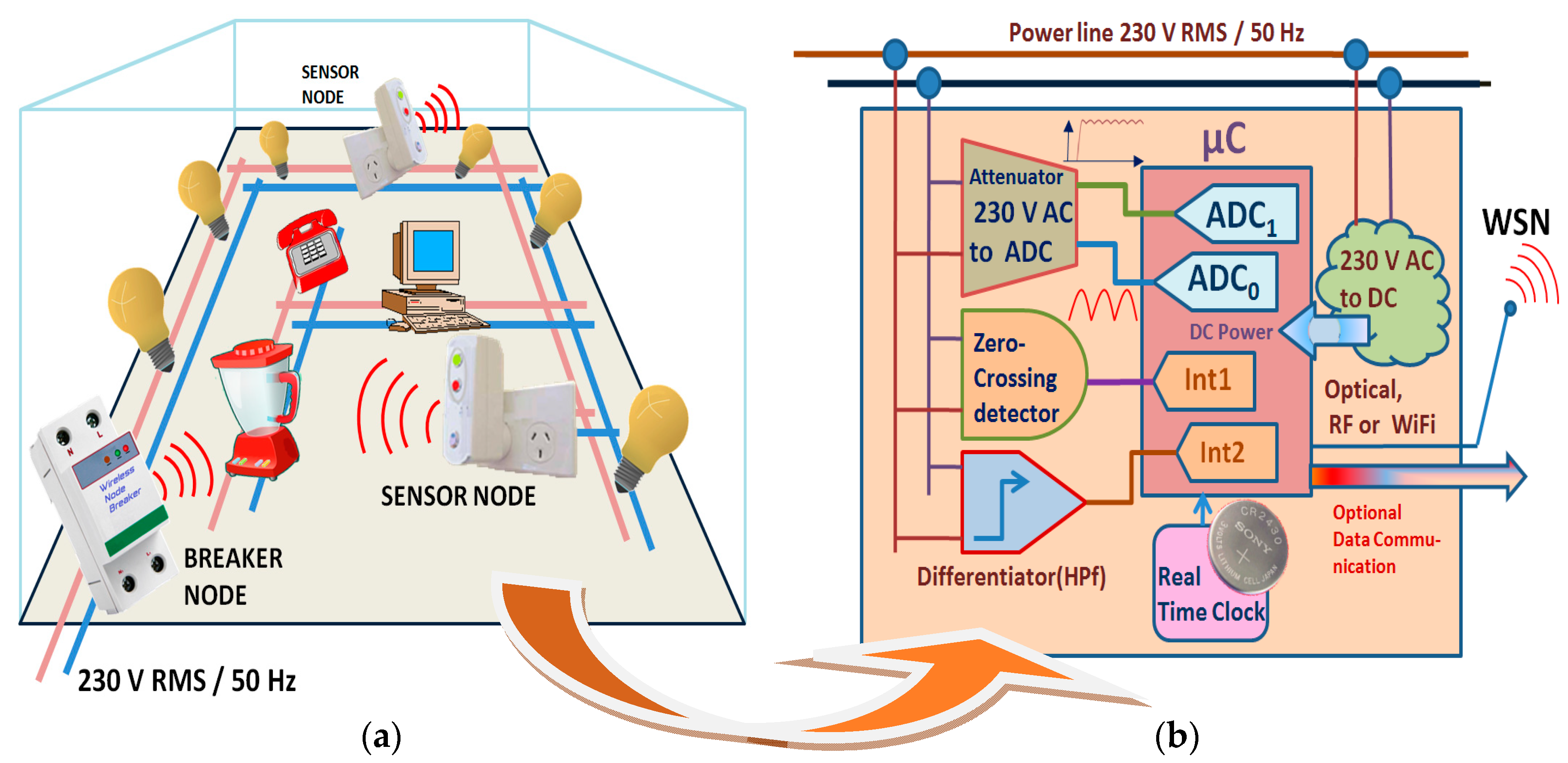
2. Sensor Node Architecture

The solution was conceived to facilitate the network installation and it consists of a sensor module connected to AC power sockets (Figure 1a). Likewise, it could be installed inside the appliances, actuating as a self-protection mechanism, disconnecting when a dangerous transient is detected. The sensor node block diagram is depicted in Figure 1b. Each node is used as a real-time failure data logger. In this case, it is compulsory to include an independent real-time clock and to provide enough memory to implement an efficient data-logger for failure reporting. Moreover, wireless data communication is required for a couple of reasons. Firstly, the complexity and the installation cost are strongly reduced. Secondly, users and processing equipment must be electrically isolated from the sensor node.

Due to the widespread use of open hardware prototyping platforms such as Beagle-Bone, Raspberry-Pi or Arduino, we adopted the ATmega328 microcontroller [29] that is also the core of the various development boards in the market. Thus, the results can run on an Arduino or an equivalent platform (assembly language directly) or on other similar processors of the same Atmel manufacturer series. It is also possible the immediate transfer to other analogous micro-controllers from other manufacturers. In addition, many sensor node platforms have also integrated ATmega devices (Waspmote, Arduino-BT, WiSmote, Tnode, NanoQplus, PanStamp, Mica, Mica2Dot, BTnode, AVRaven, Cricket, Iris, etc.) [25].

2.1. Acquiring and Conditioning of Electrical Parameters

The sensor node involves the microcontroller and its internal resources (analog-digital converter (ADC), memory, timers, interruption mechanisms and comparators). Each node is situated at one concrete point of the installation and monitors local voltage transients.

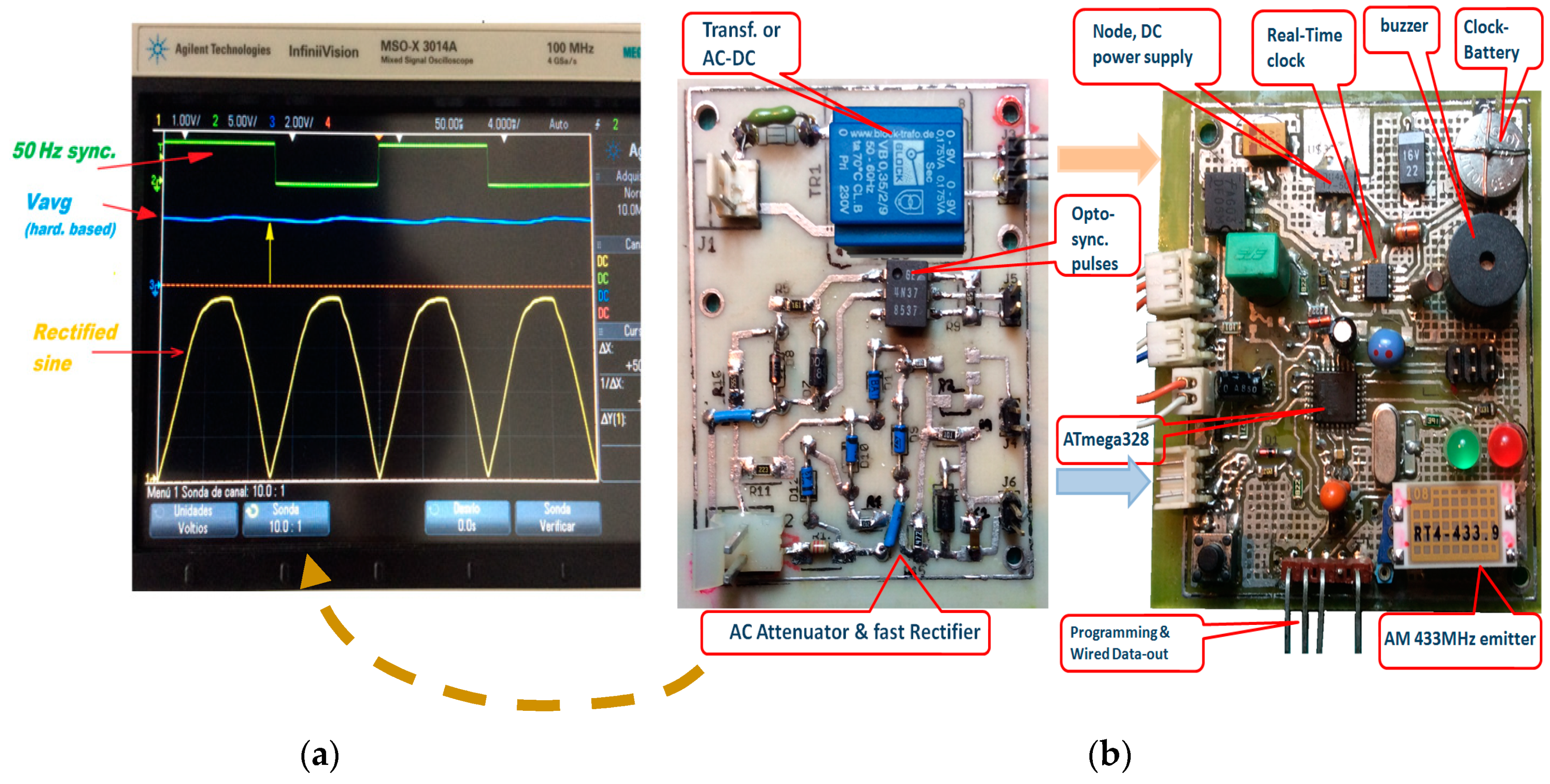
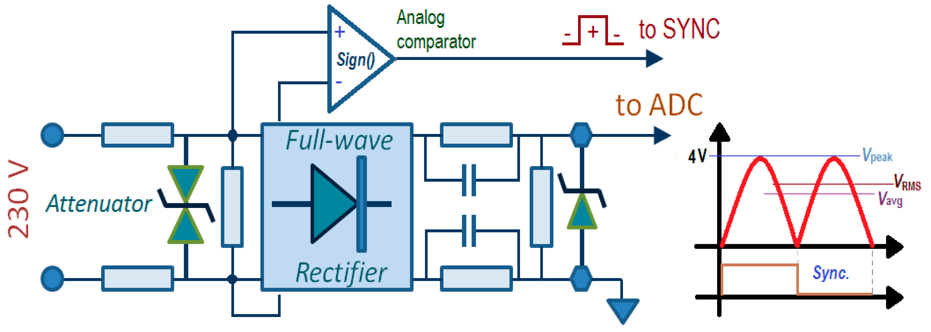
2.1.1. Alternating Current (AC) Power Line Adapter

As depicted in Figure 2, the analog-to-digital conversion (ADC) is realized from an attenuator and rectifier adaptor (adding overvoltage protection, as Transil^TM or TransZorb^TM devices). Thus, the voltage at ADC input is a scaled value, smaller with respect to the no-rectified voltage present on the AC power line. The AC voltage divider introduces an attenuation factor of 57.5. In this way, a 230 V AC is represented in the ADC by 4 V DC. Regarding the IEC 61557-12 standard, referring to root mean square (RMS) and swell and dip measurement, the ‘120% Un’ limit is equivalent to 276 V RMS. The maximum value measurable with this attenuator is 287 V RMS (ADC full scale). However, concerning IEEE STD 1159-2009, the maximum RMS voltage (swell cases) is higher than 400 V. To increase the range, a solution could be to use an additional attenuator, with a factor divider higher than 57.5 and connected to other ADC input available (e.g., a factor of around 100).

Processing from rectified voltage is proposed because the dynamic range of the ADC converter is doubled. In this sense, all the programming codes of the microcontroller will take into account the absolute value of the sinusoidal voltage, abs[V(t)], but it is necessary to know the original sign of every rectified half-wave. This function is achieved by utilizing an analog-comparator.

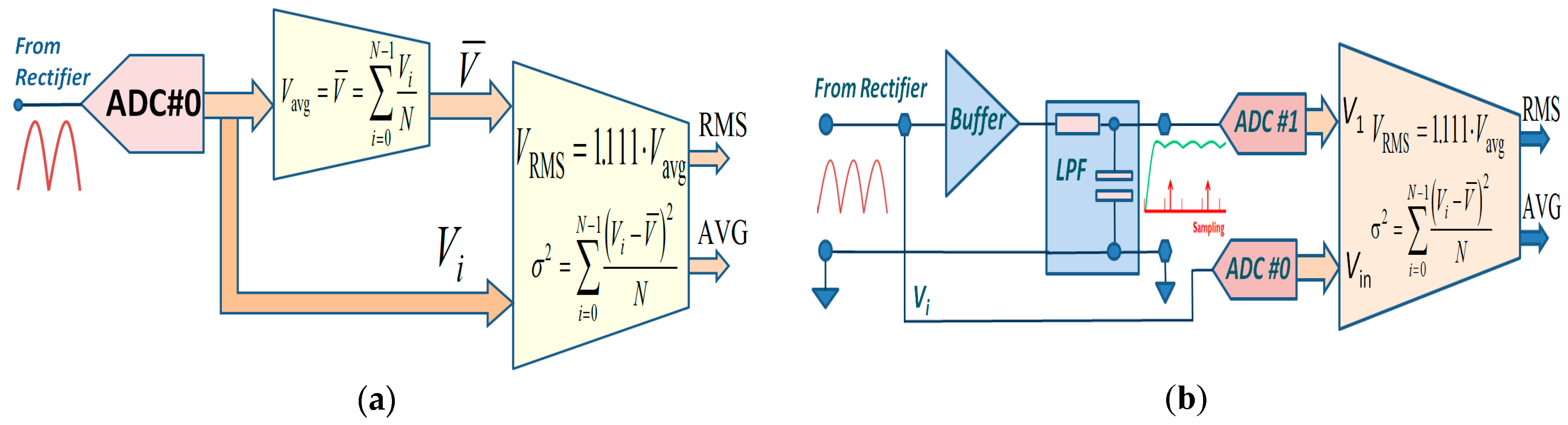
2.1.2. Average Voltage Measurement

Considering a sine-wave input, if it is applied an averaging algorithm, we can obtain the RMS value using the V_RMS and the average voltage, V_avg, ratio given by $V_{\mathrm{RMS}}/V_{\mathrm{avg}}=\pi /\left(2\sqrt{2}\right)=1.111$ (Figure 3a).

To get the arithmetic average value only a simple summation processing applied during the preceeding complete cycle is required, which for 50 Hz or 60 Hz is needed to just analyze one frame of 20 ms (50 Hz) or 16.7 ms (60 Hz). To simplify, it is not necessary to divide by N, the samples number: the final sum is just proportional with regard to N to the average amplitude. Any deformation of the signal shape will affect equally this final result and could be a failure indicator. However, to speed up the computation, it is possible to get the V_RMS and V_avg taken as the result of the peak value measurement. This value can be acquired sequentially from a second ADC (Figure 3b). We assume that the input voltage is sinusoidal, without anomalies most of the time, except during transient events.

Table 1. Different categories of interruptions (a) and disturbances (b), according to the duration of the phenomenon and their amplitude (IEEE STD 1159-2009, regarding to the 50 Hz and 230 V AC case).

a) Interruptions (Categories)	Amplitude (230 V RMS/50 Hz)	Duration	b) Transients /Disturbances	Typical Spectral	Typical Duration	Relative Duration (D) (230 V RMS/50 Hz)
Instantaneous:			Impulsive:
-Sag	207 V to 23 V	0.5 to 30 cycles or 10 ms to 0.5 s	-Short	5 ns rise	< 50 ns	T = 50 ns → D = 25×10−5%
-Swell	253 V to 414 V		-Medium	1 μs rise	0.05 to 1 ms	T = 0.5 ms → D = 2.5%
Momentary:			−10% cycle	0.1 ms	< 1 ms	T = 1 ms → D = 5.0%
-Interruption	<23 V	0.5 s to 3.0 s or 25 to 150 cycles	Oscillatory:
-Sag	207 V to 23 V		-Low freq.	<5 kHz	0.3 to 50 ms	T = 0.3 ms → D = 1.5%
-Swell	253 V to 414 V					T = 50 ms → D = 250%
Temporary:						0 to 920 V
-Interruption	<23 V	3.0 s to 1.0 min or 150 to 3000 cycles	-Med. freq.	5 to 500 kHz	20 μs	T = 20 μs → D = 0.1%
-Sag	207 V to 23 V					0 to 1840 V
-Swell	253 V to 414 V		-High freq.	0.5 to 5 MHz	5 μs	T = 5μs →D = 25×10−3%
Long duration:						0 to 920 V
-Sust. Interr.	≈0 V	>1.0 min or 3000 cycles
-Under-volt.	207 V to 184 V
-Over-voltage	253 V to 414 V

shows a list of classified phenomena according to IEEE-1159 recommendations. In the IEC 61557-12 are established test methods to assess them [4]. In general, a lot of these disturbances can be detected using time-domain methods instead of the frequency domain. On the other hand, high-frequency disturbances or oscillations require implementation of the Fourier transform or complex digital filtering, resulting in a high computational cost when we are using reduced feature processors. The evaluation of the peak and average voltage allows quick detection of some common electrical supply failures such as sag, swell and interruptions.

2.2. Signal Processing Techniques

Our goal is to achieve a compact sensor node employing minimal hard ware equipment. For this reason, the use of C++ language or machine code would allow accelerating the algorithms to real-time detection. We will focus on analyzing only easily implementable algorithms on a microcontroller-based platform. Mainly, the statistical techniques are easy to implement. Unquestionably, it is very difficult to obtain real-time FFT computed in a microcontroller with limited resources. For this reason, the selection of the algorithms must be the main purpose.

2.2.1. Statistical Processing Techniques

Frequently, statistical variables from first-order moments (such as variance and the mean) are used. This does not exclude the possibility to apply higher-order statistics (HOS) and Kurtosis procedures. However, the HOS evaluation is more oriented to harmonic analysis (spectral kurtosis) [5,6,7]. Basically, the arithmetic average value per cycle and the previous average calculated during many cycles provide information about the voltage waveform integrity and the supply continuity (interruptions). Therefore, it is possible to apply this detection method to some of the phenomena listed in Table 1a.

The application of statistical analysis requires then calculating moments over a whole period. As N (samples number) is a constant value and the sampling is synchronized every period, the variance of the rectified signal is given by:

$$\begin{array}{ccc}{\mathsf{\sigma }}^2\propto {\displaystyle \sum _{i=0}^{N-1}{\left(V_i-\overline{V}\right)}^2}& ,\mathrm{where}& V_{\mathrm{avg}}=\overline{V}={\displaystyle \sum _{i=0}^{N-1}\frac{\left|V_i\right|}{N}}\end{array}$$

(1)

The knowledge of the arithmetic average value reveals indirectly the effective total surface value of the waveform previous cycle and, thus, large voltage variations as well as micro-interruptions. It would not be applied to detect sudden transients that momentarily affect to the sinusoidal waveform. Although the algorithm is very simple, the HOS computational effort is really notable.

2.2.2. Detection Algorithm Using Kalman Filter

A Kalman filter [30] behaves as a predictive element to develop the effective comparison of the regular signal, with a momentary perturbed sine wave. This algorithm attempts to minimize the covariance error between every captured input sample and the corresponding expected output value with respect to a previous wave form.

For the prediction of the sine wave voltage given V(t) = U sin(ωt) (representing an AC voltage with U = √2 ∙ V_RMS the peak value, without disturbances), can be established as an equation in the state space considering the amplitude U(t) as the main parameter to be estimated and, secondly, the frequency variations of this waveform. In order to form a system of at least two matrix equations, we compose the orthogonal state equations according to the signal itself (sine) and 90 degrees out of phase (cosine) obtaining both equations:

$$\begin{array}{cc}\begin{array}{c}{x}_1(k)=U\sin \left(2\pi \cdot f\cdot t_k+\theta \right)\\ x_2(k)=U\cos \left(2\pi \cdot f\cdot t_k+\theta \right)\end{array}\}& \begin{array}{cc}\begin{array}{cc}& \end{array}\begin{array}{c}\mathrm{to}{t}_{k+1}=t_k+\Delta t\\ \mathrm{and}\theta =0\end{array}\begin{array}{cc}& \Rightarrow \end{array}& \begin{array}{c}{x}_1(k+1)=U\sin \left(\omega \cdot t_k+\omega \cdot \Delta t_{}\right)\\ x_2(k+1)=U\cos \left(\omega \cdot t_k+\omega \cdot \Delta t_{}\right)\end{array}\}\end{array}\end{array}$$

(2)

where ω = 2πf is the sine wave frequency, U is the estimated voltage value and x₁(k) and x₂(k), state functions at time k. In order to simplify, it can be considered an initial null delay (θ = 0). The next state (k + 1) can be established using the differential Δt, after of t_k time. By making use of the incremental time t_k+1 = t_k + Δt, x₁(k + 1) and x₂(k + 1) will be the next states. Employing trigonometric relationships for sums of sine and cosine, the Equation (2) can be simplified as follows:

$$\begin{array}{ccc}\begin{array}{c}{x}_1(k+1)=U\cos \left(\omega \cdot t_k\right)\sin \left(\omega \cdot \Delta t\right)+U\sin \left(\omega \cdot t_k\right)\cos \left(\omega \cdot \Delta t\right)\\ x_2(k+1)=U\cos \left(\omega \cdot t_k\right)\cos \left(\omega \cdot \Delta t\right)-U\sin \left(\omega \cdot t_k\right)\sin \left(\omega \cdot \Delta t\right)\end{array}\}& \Rightarrow & \begin{array}{c}{x}_1(k+1)=x_2(k)\sin \left(\omega \cdot \Delta t\right)+x_1(k)\cos \left(\omega \cdot \Delta t\right)\\ x_2(k+1)=x_2(k)\cos \left(\omega \cdot \Delta t\right)-x_1(k)\sin \left(\omega \cdot \Delta t\right)\end{array}\}\end{array}$$

(3)

and finally, we have:

$$\left(\begin{array}{c}{x}_1(k+1)\\ x_2(k+1)\end{array}\right)=\left(\begin{array}{cc}\cos \left(\omega \cdot \Delta t\right)& \sin \left(\omega \cdot \Delta t\right)\\ -\sin \left(\omega \cdot \Delta t\right)& \cos \left(\omega \cdot \Delta t\right)\end{array}\right)\left(\begin{array}{c}{x}_1(k)\\ x_2(k)\end{array}\right)$$

(4)

Since the output variable of interest is precisely the state x₁(k), the equation indicating the measured value output, z(k), is exactly the state x₁(k) itself and the superimposed noise υ(k):

$$z(k)=\left(\begin{array}{cc}1& 0\end{array}\right)\left(\begin{array}{c}{x}_1(k)\\ x_2(k)\end{array}\right)+\upsilon (k)$$

(5)

where υ(k) is white noise with null mean value. When a transient is superimposed, then this disturbance υ(k) is now not Gaussian, which causes discrepancy with respect to the previously estimated voltage. The Kalman filter allows a sufficient prediction of sinusoidal voltage from the previously sampled data. By comparing a recently sampled period with abnormalities (disturbances) with a previously predicted sine wave without apparent irregularities, it will generate a differential value when detecting any mismatch between the two periods (with and without transient pulses).

2.2.3. Detection Algorithm Using the Helmholtz Equation

Given that function V(t) = Usin(ωt) representative of the AC power line is an n-times differentiable function, it is possible to set it into an one-variable ordinary differential equation, as the one-dimensional Helmholtz mathematical expression, and this can by written as:

$$F=f^{″}(t)+K\cdot f(t)=0$$

(6)

Annulment of F in Equation (6) is a method to find variations of f(t) when this function is a periodic signal such as the analyzed sine wave. The proof is obvious in the linear version case of F: given f(t) = Usin(ωt), we only need to derive the sinusoidal function consecutively to reach the conclusion that K = ω; under normal conditions, the contrasting of the sine function with its second derivative yields a null value. Once a value of K has been found for the undistorted sinusoidal function, any shape deviation with respect to the original (due to some disturbance) will affect to the function f(t) which will not be now a perfect sine wave, and consequently, Equation (6) is not verified.

When a discrimination threshold appropriate is exceeded, an alarm signal is notified announcing the disturbances presence. For the discrete case, utilizing the discrete-time variable (t→Δt) and where is now applied the voltage V(n∙Δt) = Usin(ω∙n∙Δt), with peak value U = √2 ∙V_RMS, without disturbances, for every instant n = 0,1,2,…. the derivative function is given by:

$$f\mathrm{n}(t)=\frac{U\left[\sin \left(\omega \cdot \left(t+\Delta t\right)\right)-\sin \left(\omega \cdot t\right)\right]}{\Delta t}=\frac{U}{\Delta t}\left[\sin \left(\omega \cdot t+\omega \cdot \Delta t\right)-\sin \left(\omega \cdot t\right)\right]$$

(7)

and the second derivative function:

$$f\mathrm{n}\mathrm{n}(t)=\frac{U}{\Delta t}\left[\frac{\left(\sin \left(\omega \cdot t+\omega \cdot \Delta t+\omega \cdot \Delta t\right)-\sin \left(\omega \cdot \Delta t+\omega \cdot \Delta t\right)\right)-\left(\sin \left(\omega \cdot t+\omega \cdot \Delta t\right)-\sin \left(\omega \cdot t\right)\right)}{\Delta t}\right]$$

(8)

which can be simplified in the following expression:

$$f^{″}(t)=\frac{U}{{\left(\Delta t\right)}^2}\left[\sin \left(\omega \cdot t+2\omega \cdot \Delta t\right)-2\sin \left(\omega \cdot t+\omega \cdot \Delta t\right)+\sin \left(\omega \cdot t\right)\right]$$

(9)

Applying the equality expressed in Equation (6), we have:

$$f^{″}(t)-Kf(t)=\frac{U}{{\left(\Delta t\right)}^2}\left[\sin \left(\omega \cdot t+2\omega \cdot \Delta t\right)-2\sin \left(\omega \cdot t+\omega \cdot \Delta t\right)+\sin \left(\omega \cdot t\right)\right]+KU\sin \left(\omega \cdot t\right)=0$$

(10)

If we consider K = −1, the function is canceled when the two terms are equal, or expressed otherwise, the function g(t) given by:

$$g(t)=\frac{1}{{\left(\Delta t\right)}^2}\left[\sin \left(\omega \cdot t+2\omega \cdot \Delta t\right)-2\sin \left(\omega \cdot t+\omega \cdot \Delta t\right)+\sin \left(\omega \cdot t\right)\right]\equiv \sin \left(\omega \cdot t\right)$$

(11)

that is, equal to sin(ω∙ t), which is equivalent to the initially sine wave function. Therefore, when the original f(t) slightly differs from an ideal sin(ω∙t) function, the homologous, g(t), will not verify the sinusoidal relationship. Since sin(w∙t) represents a previous cycle sampled from the next sin(ω∙(t + Δt)), we can express the function g(t) as an equation in differences, G(n), with a sampling interval (n∙Δt) of the acquired power sequence V(n∙Δt) that can be rewritten as:

$$\begin{array}{ccc}V(n)=U\sin \left[\omega \cdot \left(n\cdot \Delta t\right)\right]& \Rightarrow & G(n)=V(n+2)-2\cdot V(n+1)+V(n)\end{array}\equiv (\Delta t^2)\cdot V(n)\approx 0$$

(12)

where Δt = 1 / F_S is a very small number. Using the Z⁻² operator, the definitive equation to be algorithmically implemented is:

$$G_1(n)=V(n)-2\cdot V(n-1)+V(n-2)\approx 0$$

(13)

2.2.4. Detection Algorithm by Contrasting with Successive Previous Integrations

If during a long time interval, the acquired sinusoidal input is integrated (each sample with its respective previous one of similar phase), the V_acc[n] array of the resulting waveform should contain a filtered AC power sine wave without any transient.

$$\begin{array}{ccc}{V_{\mathrm{acc}}(n)|}_{\mathrm{current}}=\begin{array}{cc}\frac{1}{2}\left[V_i(n)+{V_{\mathrm{acc}}(n)|}_{\mathrm{previous}}\right]& \end{array}& n=0,1,2,\dots ,N& \end{array}$$

(14)

Now, if the power line is unexpectedly affected (transients, disturbances, etc.) different instantaneous input samples, V_i(t), will differ with respect to the previous arithmetic averages, V_acc(t), for those same array indexes. These differences can detect any anomaly when implementing this comparison algorithm:

$$\begin{array}{cccccc}If& \left|V_i(n)\right|-{\left|V_{acc}(n)\right|}_{n=0,1,2,\dots ,N}& >& \mathrm{threshold}& \Rightarrow & \mathrm{Transient}/\mathrm{disturbance}\end{array}$$

(15)

3. Hardware Platform

Our contribution is a low-cost and compact sensor circuit. Therefore, it is required to use the smallest number of components. The prototype has a small size (two cards, staked, 80 × 60 mm) that can be inserted into a plastic box and directly connected to the electrical socket. This purpose suggests designing an optimized hardware platform, capable of detecting disturbances in real time and avoiding the inclusion of specific integrated circuits. This sensor node is mainly oriented to measure the voltage of the power line directly using a balanced AC voltage divider. The circuit is auto-powered by the same power line where it performs the monitoring work (Figure 4b) and optionally, it can integrate supercapacitors to provide autonomy in long interruption failures.

The processor ATmega328 from Atmel (up to 20 millions of instructions per second (MIPS) is adequately fast for that price range) has been selected. This integrated circuit is the core component of the Arduino prototyping platforms. This choice allows us to translate the validated conclusions from our prototype toward others similar open hardware platforms. A real time clock (Maxim DS1307 powered by a back-up battery) drives the timing for the failure data-logger. The prototype also includes a buzzer and two light-emitting diodes (LEDs) to show the current state of the node and to alert of any recent failure.

A wireless communication emitter (AM modulation at 433 MHz) is added to transmit the results. Optionally, a BlueTooth or WiFi module can be connected. This communication method allows the formation of the network and the galvanic isolation since the modules work directly with the AC line voltage. Additionally, an infra-red communication receiver has been included only for purposes of wireless configuration from a computer. A second circuit board contains the attenuators, edge detector (synchronism), rectifier and equalizer for the direct measurement of the main power voltage. Both cards are connected in a sandwich mode (stacked) to reduce the overall size of the equipment and achieve greater galvanic isolation from the AC power card.

In order to avoid electric risk during the preliminary debug and tests, a transformer has been inserted to isolate the main power voltage and it allows direct connection from the prototype to the computer, through the universal serial bus (USB) port.

3.1. Measurement Setup

The sensor node must be connected directly to main power line. The attenuator adapts the AC power voltage to the microcontroller ADC converter. Figure 4a shows an oscilloscope image of the rectified sine wave (yellow) at the ADC input. This ADC voltage is scaled over 4 V peak when a 230 V RMS nominal voltage is present in the power line. It can also be seen the sync pulses (green, every zero crossing) and the peak value, V_peak, using hardware method (rectifier and RC-filter).

3.1.1. Dynamic Range

Dynamic range is optimized for the ADC full-range (10 bits and 5 V DC input max) to represent the rectified full-wave. It is planned that this maximum ADC range, 5 V, represents a 25% higher input than the service voltage (230 V AC previously scaled by the input attenuator, see Figure 2) and 287 V RMS (ADC full scale).

With this factor, we have 4 V DC (equivalent 230 V AC) into the ADC converter. Regarding the IEC 61557-12 standard, the ‘120% Un’ limit referred to is equivalent to 276 V RMS. For specified cases in IEEE-1159 (Table 1) as swell and over-voltage, this recommendation considers a maximum amplitude of 1.8 p.u., that regarding 230 V power line, can estimate shall rise around 414 V RMS (or 585 V peak). This will develop a peak value into the AD converter of 7.2 V (the maximum permissible ADC input level is 5 V). Therefore, a Zener protection circuit must limit it to a maximum voltage of 5.1 V. Voltage peaks above the 1.25 p.u. will not be evaluated quantitatively by our detector (only qualitatively). In Section 2.1.1, an optional measurement range increase is proposed.

3.1.2. Synchronous Conversion and Sampling Rate

The conversion synchronized every zero crossing of the input voltage avoids the requirement of windowing techniques and leads to simple comparisons of 256 samples per block, sequentially captured every period. Thus, similar samples successively occupy the same phase locations in a conversion data array (a solution already proposed by Artioli et al. [16]). The crossing detection is very easy using an analog-comparator or an opto-coupler. This provides constantly an array size of N = 2⁸ = 256 numbers in all applied algorithms. Therefore, the conversion speed is set to 256 samples per period of the input voltage (50 or 60 Hz). This quantity is a compromise between resolution and memory size, and affects both data arrays of samples and of intermediate results. For a power line of 50 Hz, this supposes a sampling rate F_S = 256 × 50 Hz = 12.8 kHz. This frequency allows an accurate representation of the full-wave rectified sine wave of 50 Hz, but limits the bandwidth of transients at about 6.4 kHz according to Nyquist limit.

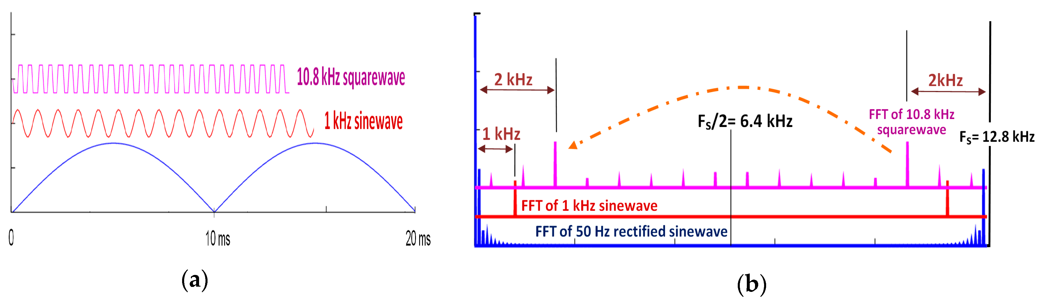
3.1.3. The Absence of the Anti-Aliasing Filter

For simplicity, the essential anti-aliasing filter was not included in the data acquisition sequence. Since the monitor mission is to detect disturbances qualitatively, we expect to capture easily high-frequency transients outside the Nyquist range. We take advantage of the overlapping phenomenon (a consequence of Shannon’s theorem itself) considering the mirrored copies of the higher spectral components, to the low side, with respect to the sampling frequency point, F_S.

Thus, any high-frequency transient that exceeds the requirements of band-pass framed below Nyquist frequency, F_S (e.g., some perturbation frequencies above of F_S/2 = 12800 Hz / 2 = 6400 Hz) should generate errors in the conversion process and shall appear as spectral components into the sampling frequency band due to overlap effect (lower sideband in a heterodyning phenomenon, Figure 5). Consequently, this mirrored component, below than F_S frequency, can also reveal the disturbances.

By Shannon’s theorem (graphically expressed in Figure 5), generally if aliasing exists, the transient component located above F_S/2 is now reflected in the Nyquist sampling area, within the spectrum band conversion between 0 Hz and F_S (overlap). Under these circumstances, some disturbance components will be qualitatively processed and the algorithms can indicate the presence of anomalies. However, although this simplification allows detection of transient pulses above the sampling frequency, cannot correctly determine the event frequency: it is only possible to determinate that this disturbance had occurred.

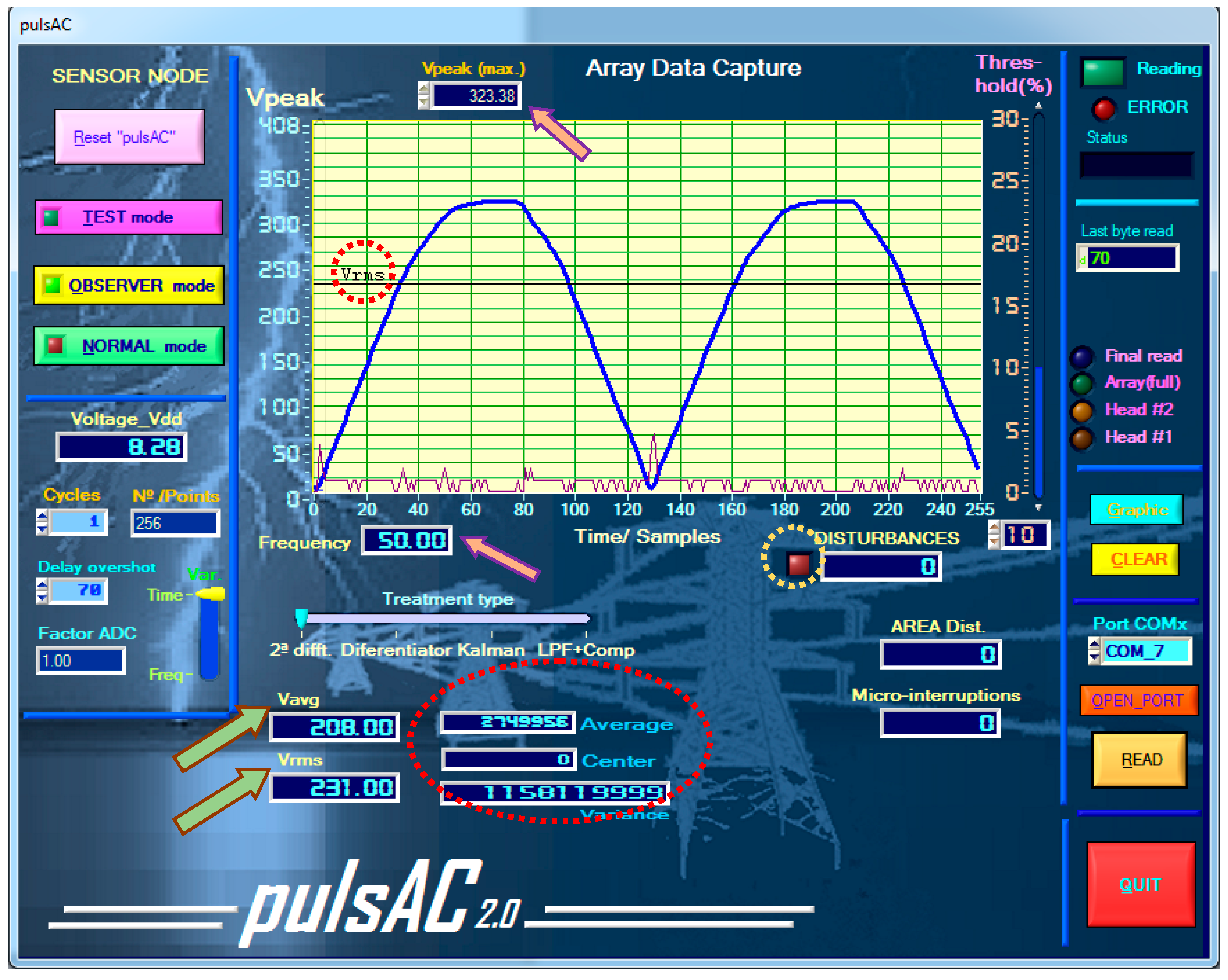
3.1.4. Application Software for Essays of Algorithms and Test-Bench

An application called ‘puls.AC’ was developed to verify the algorithm implementations and the prototype electronic board (Figure 6). This software tool has been programmed in C++ language employing the LabWindows/CVI environment from National Instrument^TM. If the procedures are written using exclusively an integer-numbers based programming code, the detection algorithms can be directly translated and tested in assembler language for ATmega328 processor (Atmel™ company also provides a C free compiler for the developer community using its own microcontrollers).

3.1.5. Data Acquisition State Machine

To maximize the processing speed, a fast state machine was implemented using the incorporated features into the microcontroller, mainly the internal interrupting architecture. The acquiring process starts every detected zero crossing. An internal clock counter is configured to generate software interruptions during an equivalent time to the sampling period. This interruption routine forces the system to acquire an input voltage sample and save it. A counter variable allows for the conversion of a frame of up to 256 sampled data. The available free time between adjacent-acquisitions permits the processor to run the required detection algorithms (Figure 7). When the synchronism is different to 20 ms (50 Hz), the internal counter generates a count overflow. This event marks an anomaly situation.

3.2. Algorithms’ Implementation Codes

Three computational strategies have been considered:

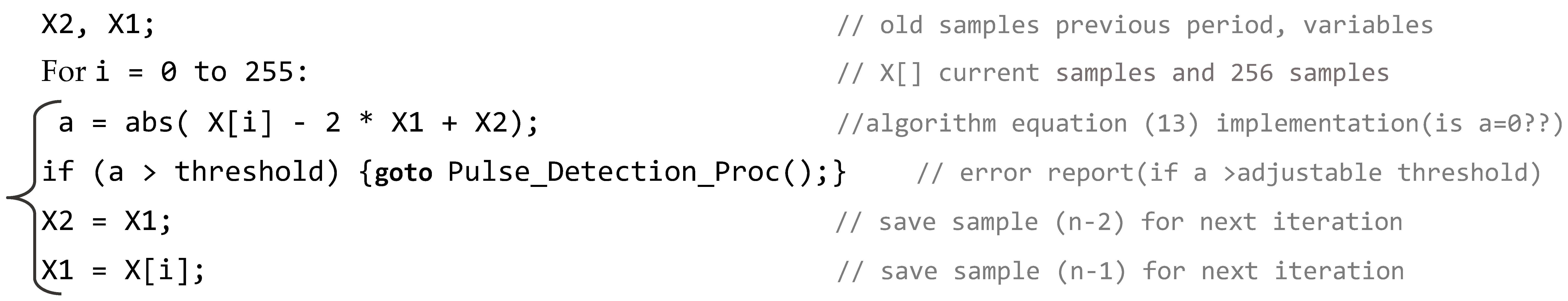
3.2.1. Detection Algorithm Based on the Helmholtz Equation

In this case, it was implemented the comparison algorithm of the second derivative of the input sine wave sampled. For a given sampling rate of Δt = 78.12 μs, is Δt² ≈ 0. The method was previously exposed and here is implemented (pseudocode) according to the conclusion given by Equation (13):

where the X[i] array contains N = 256 ADC samples captured during an interval of T = 20 ms (50 Hz period); thereby it is Δt = 78.12 μs.

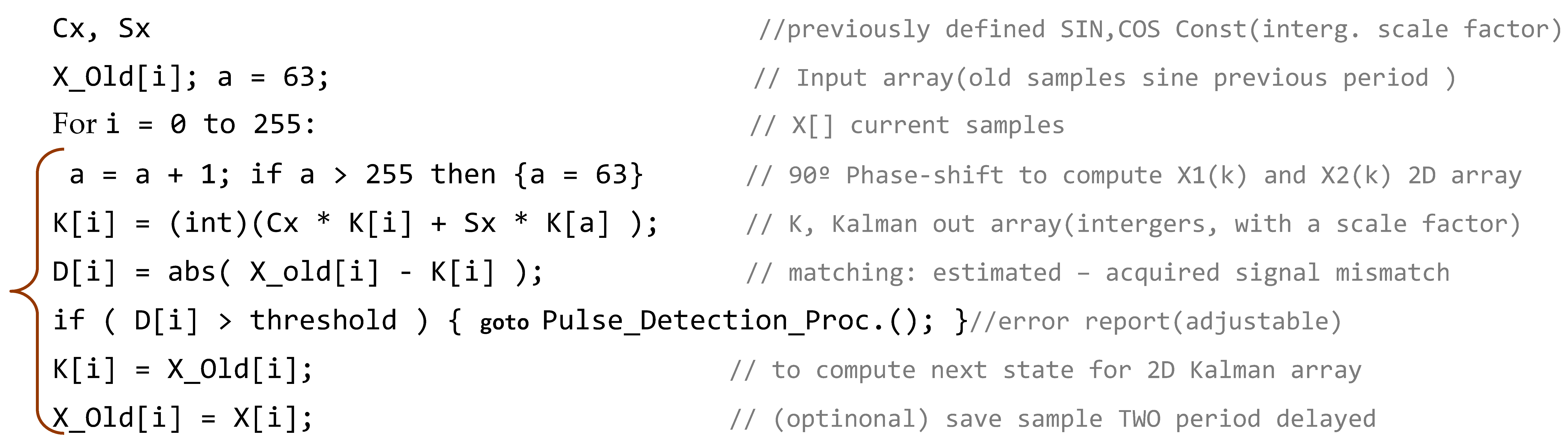
3.2.2. Kalman Filter Implementation

As discussed in Section 2.2.1., the minimized Kalman filter to estimate simply amplitude A of the sinusoid Asin(ω∙t), leads to the implementation of Equations (4) and (5), implementing the following pseudocode sequence:

where, X[i] is the array of the input voltage sampled, and Cx, Sx, the coefficients of the resulting Kalman-2D array for sinusoidal prediction case (3). The K[i] array are estimates of the ideal sine wave (without interference) and are compared with the X[i] array, resulting in the differences array, D[i]. Three arrays are required: one to contain the instantaneous samples input voltage (256 words) and two more to the consecutive previous periods (512 words); two fixed-point multiplications are required too.

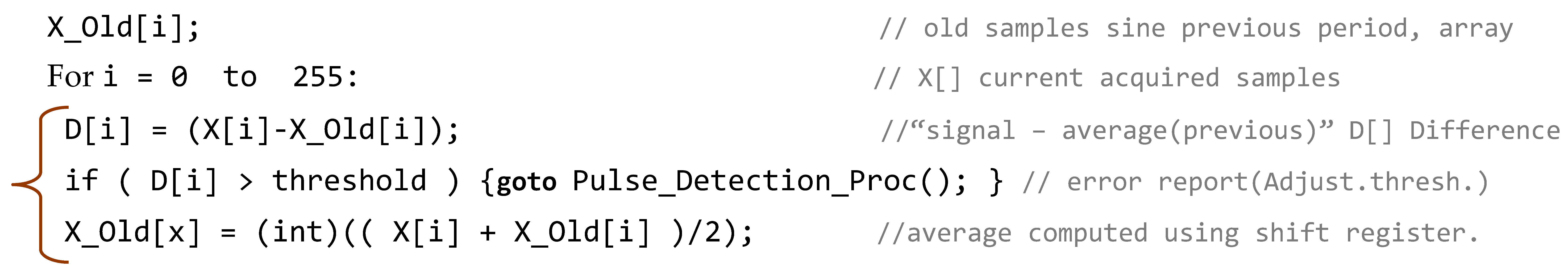
3.2.3. Detection Algorithm by Contrasting with Successive Previous Integrations

This method was previously shown and requires the successive integration of the input sine-wave captured. In fact, an averaging algorithm successively and repeatedly applied to a sinusoidal voltage with transients leads towards a pure waveform without disturbances. Every voltage sample newly acquired is compared continuously with the accumulative previous average value, with an identical phase, by making use of the expression:

$$D\left[i\right]=X\left[i\right]-\overline{X}\left[i-256\right]$$

(16)

where X[i] is the current samples array and $\overline{X}\left[i-256\right]$ contains the average samples of previous periods. The general equation for any integration algorithms is $\overline{X}\left[i\right]=\left(X\left[i\right]+X_{old}\left[i\right]\right)/\beta$. This algorithm acts as a low pass filter and can to remove any previous transient. For this case, we have used the averaging formula (X[i] + X_old[i]) / 2, since it is easier compute a base-2 binary division that can be solved with a simple shift to the left, following the addition. The basic pseudocode is:

4. Results

To verify the sensor-node prototype performance and to check the different detection algorithms, three routines only were implemented. Therefore, a basic set of different transient pulses and oscillations has been applied according to some conditions included in the IEEE-1159 recommendation (Table 1). Specifically, the Helmholtz equation method, the Kalman predictor, and the successive integration (LPF) and comparison method have been compared. These three techniques have shown that they are easily implementable and give an efficient response to the failure detection.

To generate real transients, we used a standard analog function generator Tektronix CFG250 and an ad-hoc circuit board with manual switches (Figure 8) that allow us to enter the following scaled disturbances:

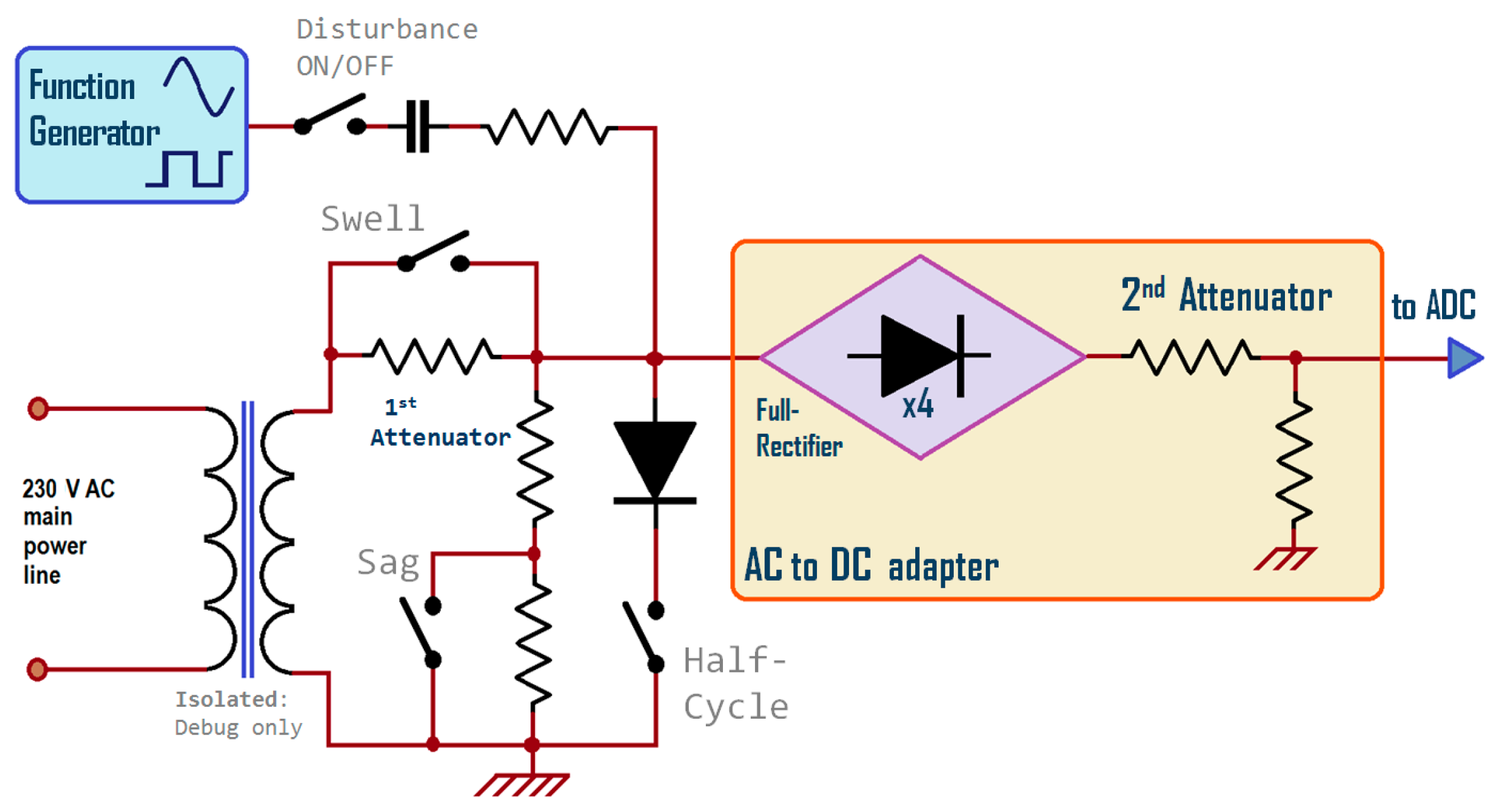
• V_RMS decreased by approximately half of the nominal 230 V AC (−54.7%) (0.6 p.u. momentary sag).
• Half-cycle missing or a sag in an amount bigger than 10% (instantaneous sag, 0.5 cycles > 0.1 p.u.).
• Swelled peak voltage at 13.35% over the 311 V nominal peak (1.13 p.u. momentary swell).
• Permanent or intermittent disturbance signals, as sine or square waves, with different amplitude levels and frequencies, from the function generator.
• To emulate impulsive transients of different duration, square pulses of low, medium and high frequency (10 Hz, 1 kHz, 10 kHz and 100 kHz) and amplitude up to 10% of V_peak (corresponding to 0.1 p.u., with respect to the rectified voltage and using a voltage divider) were injected. To emulate harmonic distortion a 200 Hz sine low-amplitude component can also be superimposed. Different sinusoidal functions (10 Hz to 10 kHz), approximately 10% (0.1 p.u.) amplitude with respect to the rectified voltage peak value were used for oscillations simulation.

The adjustable ‘threshold’ level permits us to modify the failure detection sensitivity. To achieve the maximum, sensitivity should be taken to the lowest level possible, but avoiding the occurrence of false alarms.

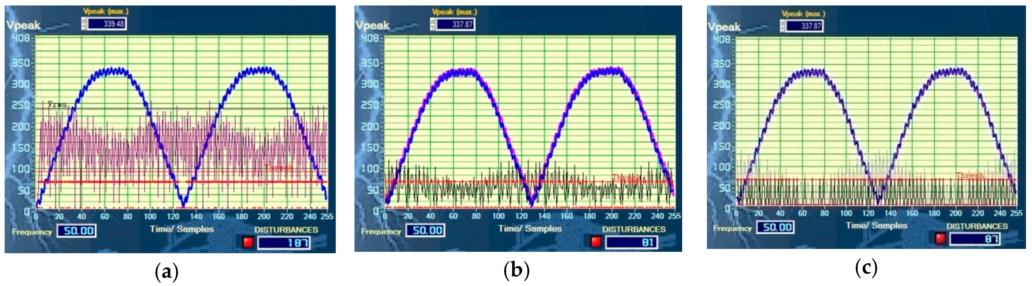
4.1. Helmholtz-Based Method

• Voltage fluctuations testing: the slow voltage variation generates small differences values in the derivative algorithm given by Equation (13). This method is insensitive for phenomena such as sag or swell voltage.
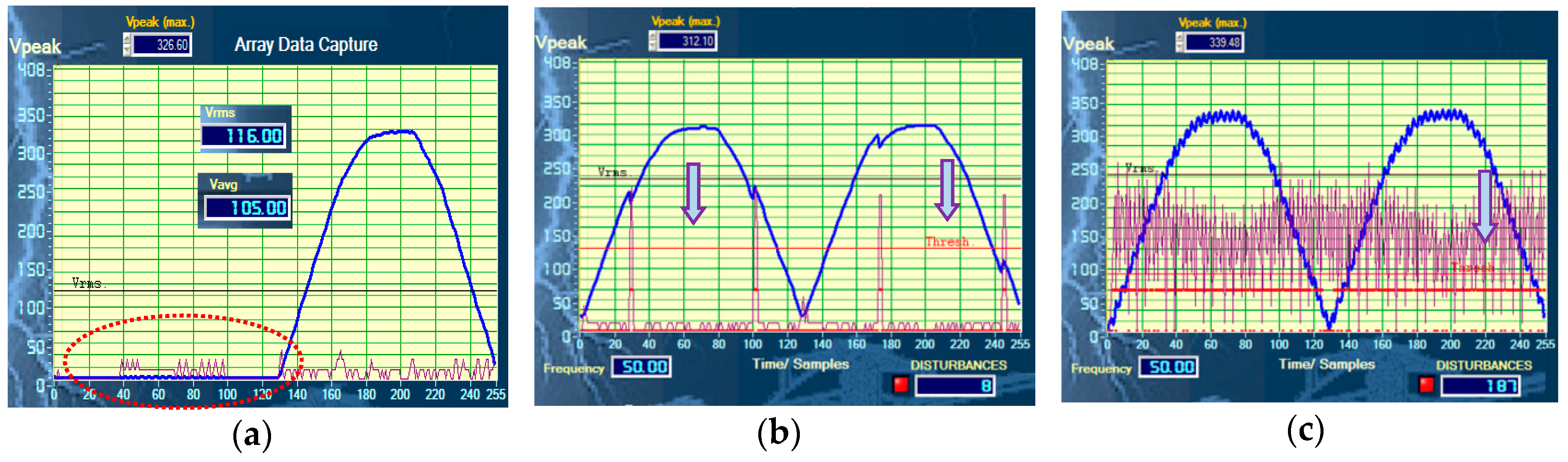
• The process is not sensitive to brief changes such as micro-interruption or sudden half-cycle missing failures (Figure 9a) because the algorithm requires a full period to compute completely the array of the sampled input voltage.
• When a square voltage (1 kHz or 100 Hz) is superimposed (Figure 9b) the algorithm presents a good detection response (relative threshold = 5% adjustable from 0 up to 30%). It also works correctly for high frequencies (10 kHz and 100 kHz, even greater than F_S (Section 4.4)

To detect up to 1 kHz order sinusoidal oscillation injected, it is necessary to decrease the detection threshold up to 2%. This causes any false alarms even when the AC voltage is normal (undistorted). In this situation, it is impossible to detect the 4th harmonic distortion using this method. However, it works properly for higher frequencies (as 10 kHz and 100 kHz > F_S) (Figure 9c).

4.2. Kalman Filter Detection

• Voltage fluctuations testing: Figure 10a shows a half-cycle sudden failure (blue). Thus, the filter predicts the half-cycle missing (magenta) and consequently detects the failure (the green line show the error value; the red one is the computed comparator result). Likewise, it also detects slow disturbances with a presence for a longer time than the period of the signal.
• Since detection is a strategy based on prediction, the code correctly detects the square transients (Figure 10b). When a square wave voltage is superimposed (frequencies of 10 Hz to 1 kHz), the algorithm presents a good differentiation (up to a relative threshold level of 6%, adjustable).
• Injecting a sine wave disturbance higher than 10 Hz, the system shows a good response, for different threshold values (Figure 10). In this case, it is possible to detect the harmonic distortion (4th-harmonic of the 50 Hz sine wave).

4.3. Method of Successive Integrations (LPF) and Comparison

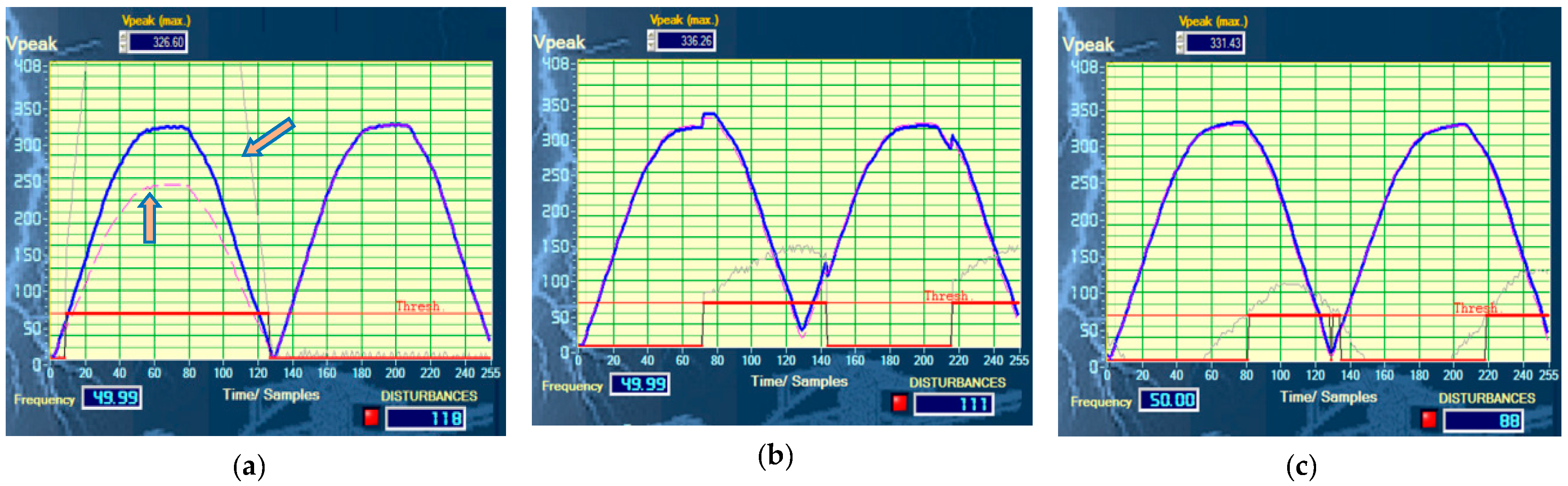
• Voltage fluctuations testing: since the algorithm obtains an arithmetic average of each similar phase sample (during previous periods), this process is slow with respect to any very fast event that may occur in the immediate preceding half-cycle. In these situations, sometimes the algorithm can produce an erroneous result. However, since the final average is obtained from the immediately previous samples, it works quite accurately when sudden events occur, lasting longer than a half-cycle. In this case, a swell voltage variation is detected perfectly.
• This method works properly when a square disturbance is injected (Figure 11b). For square wave voltage superimposing tests (10 Hz and 1 kHz), the algorithm presents a good differentiation and detection (using a threshold level of 6%). If the phenomenon is persistent, the transient will gradually dissolve in the averaged waveform array (due to the filter effect).
• For low-frequency sinusoidal oscillation (hundreds of Hz), the procedure has an equally good detection response because it compares the current signal samples with the previous averaged sine wave and without transients (Figure 11c). It could also detect the harmonic distortion (presence of the 4th harmonic).

4.4. Performance in High Frequency

To verify the effectiveness of the ADC and sampling bypassing the antialiasing filter, we compare results of the three previous algorithms, considering an oscillation injected of 10 kHz, near to sampling frequency (Figure 12). The response was also good for the highest frequencies (up to 100 kHz).

Table 2. The response of the different algorithms analyzed.

Disturbance	Helmholtz Equation	Kalman Filter	Successive Integrations and Comparison
Sag/Swell	NO, False detections	Yes	Yes
Half-cycle off	NO, False detections	Yes	NO, slow for half-cycle
Pulse 100 Hz/10%	count any sudden pulses	Yes	Yes
Pulse 1 kHz/10%	Yes	Yes	Yes
Pulse 10 kHz/10%	Yes	Yes	Yes
Oscillation 200 Hz/10%	No sure detection (low freq.)	Yes	Yes
Oscillation 1 kHz/10%	Yes	Yes	Yes
Oscillation 10 kHz/10%	Yes, best if F > F sampling	Yes, work F > F sampling	Yes, work to F > F sampling

summarizes the different results for each method discussed in this paper. Attending to the results, the Kalman algorithm has a better transient detections response. However, it represents a slight implementation complexity compared to other implemented algorithms.

The integration (LPF) and comparison method requires several previous integrations cycles to a precise detection. For this reason, it works incorrectly in half-cycle disruption failures. For this case, it is easy to implement an additional algorithm based on peak value measurement.

Similarly, the Helmholtz-based method does not detect voltage variations cases. Any additional algorithm can be used to mathematically analyze the peak voltage variations.

5. Conclusions

This work presents a low-cost sensor-node supported on a microcontroller platform. It is aimed to be integrated into a cooperative wireless sensor network. In order to simplify, an attenuator-rectifier adapter was proposed to connect the analog-to-digital converter to the power line. The rectifier process improves the dynamic range of the ADC, but introduces a low-intensity spectral content in 200 Hz and with lower intensity, in 400 Hz.

Several simple processing algorithms were also analyzed, implemented and tested to assess the transient detection capability and specific oscillation failures (PQ). In order to accelerate the computational work, it was essential to execute integer mathematical algorithms. The search and selection of implementable algorithms and real-time achievement is an additional difficulty. Therefore, these small integrated systems could act correctly as very low-cost and low-power instruments to become sensor nodes. Frequency, RMS voltage and transient voltage measurements are feasible. The ADC (10 bits) resolution could comply with some standards as a lot of IEC-61557-12 specific paragraphs. As the hall sensor was not included, it is not achievable at current or power measurements. However, the feature of simplicity makes them ideal parts of a PQ wireless sensor network.

In addition, a physical prototype based on an ATmega-328 microcontroller was built to verify the ideas and machine codes previously considered. It can also affirm that the use of embedded resources in simple microcontroller devices (ADC, interrupt vectors, counters, etc.) improves real-time execution performance. This prototype allows us to verify numerous detector algorithms and if necessary, we could replace the microcontroller architecture (e.g., replace ATmega by an ARM processor).

A software application (C++, LabWindows^TM) was developed and employed as an algorithms test-bench. Thus, it was possible to test the different detection methods described in this paper and to check the efficiency of each algorithm.

With this help, and as evidenced in Table 2, it can be considered that:

• In order to achieve a high penetration of sensor nodes, low-cost platforms are essential.
• For this reason, a special design is required, choosing low-energy and inexpensive hardware ad-hoc platforms and implementing specific algorithms to maximize the device performance.
• The 2nd-derivative Helmholtz method is quite sensitive to high-frequency interferences (brief oscillations) or pulses, while it is very insensitive to slow changes (harmonic distortion, sag or swell voltage).
• The Kalman filter option is the most effective and is able to show all kinds of anomalies that have been tested. The disadvantage is that it demands more memory and requires much more code implementation complexity.
• The ‘integration (LPF) and comparison’ method detects correctly for slow voltage variation or high-frequency disturbances (swell, sag, oscillations or short pulses, etc.). However, it is not capable of detecting short voltage variations with a shorter duration of a half cycle due to the integration time.

Future works may be conducted to complete the sensor network, increasing the number of nodes, to exploit the individual measurements acquired. It would also be interesting to design a breaker-node (remotely controlled) that disconnects a local section when an excessive phenomenon occurs and is detected by a remote sensor-node. In this way, this node could disconnect the power when another sensor node detects an anomaly (via radio 433 MHz).

Moreover, specific pattern recognition techniques may be considered for increasing nodes measurement capability and prediction. Thus, the node could allow predicting some anomalies.

References

1. IEEE Std. 1159-2009, IEEE Recommended Practice for Monitoring Electric Power Quality; IEEE: Piscataway, NJ, USA, 2009. [Google Scholar]
2. IEC 61000-4-30. Electromagnetic Compatibility (EMC), Part 4: Testing and Measurement Techniques. Section 30: Power Quality Measurement Methods; International Electrotechnical Commission, IEC Central Office: Geneva, Switzerland, 2008. [Google Scholar]
3. Neumann, R. The importance of IEC6100-4-30 Class A for the Coordination of Power Quality Levels. In Proceedings of the 9th International Conference Electrical Power Quality and Utilization, Barcelona, Spain, 9–11 October 2007. [Google Scholar] [CrossRef]
4. IEC 61557-12. Electrical Safety in Low Voltage Distribution Systems up to 1000 V a.c. and 1500 V d.c. - Equipment for Testing. Measuring or Monitoring of Protective Measures - Part 12: Performance Measuring and Monitoring Devices (PMD), 2nd ed.; International Electrotechnical Commission, IEC Webstore: Geneve, Switzerland, 2018; Available online: https://webstore.iec.ch/publication/64047 (accessed on 22 April 2019).
5. González de la Rosa, J.J.; Sierra-Fernández, J.M.; Palomares Salas, J.C.; Aguera Pérez, A.; Jiménez Montero, A. An application of spectral kurtosis to separate hybrid power quality events. Energies 2015. [Google Scholar] [CrossRef]
6. González de la Rosa, J.J.; Aguera Pérez, A.; Palomares Salas, J.C.; Florencia-Oliveiros, O.; Sierra-Fernández, J.M. A dual Monitoring Technique to detect Power Quality Transients Based on the Fourth-Order Spectrogram. Energies 2018, 11, 503. [Google Scholar] [CrossRef]
7. Palomares Salas, J.C.; González de la Rosa, J.J.; Sierra-Fernández, J.M.; Aguera Pérez, A. HOS Network-based classification of power quality events via regression algorithms. EURASIP J. Adv. Signal Process. 2015. [Google Scholar] [CrossRef]
8. Valtierra-Rodriguez, M.; De Romero-Troncoso, J.; Osornio-Rios, R.A.; Garcia-Perez, A. Detection and classification of single and combined power quality disturbances using neural networks. IEEE Trans. Ind. Electron. 2014, 61. [Google Scholar] [CrossRef]
9. Borges, F.A.S.; Fernandes, R.A.S.; Silva, I.N.; Silva, C.B.S. Feature Extraction and Power Quality Disturbances Classification Using Smart Meters Signals. IEEE Trans. Ind. Inform. 2016, 12, 824–833. [Google Scholar] [CrossRef]
10. Zygarlicki, J.; Zygarlicka, M.; Mroczka, J.; Latawiec, K.J. A Reduced Prony’s Method in Power-Quality Analysis Parameters Selection. IEEE Trans. Power Deliv. 2010, 25. [Google Scholar] [CrossRef]
11. Liu, Z.; Cui, Y.; Li, W. Combined Power Quality Disturbances Recognition Using Wavelet Packet Entropies and S-Transform. Entropy 2015. [Google Scholar] [CrossRef]
12. He, S.; Li, K.; Zhang, M. A Real-Time Power Quality Disturbances Classification Using Hybrid Methods Based on S-Transform and Dynamics. IEEE Trans. Instrum. Meas. 2013, 62. [Google Scholar] [CrossRef]
13. Dash, P.K.; Chilukuri, M.V. Hybrid S-Transform and Kalman Filtering Approach for Detection and Measurement of Short Duration Disturbances in Power Networks. IEEE Trans. Instrum. Meas. 2004, 53. [Google Scholar] [CrossRef]
14. Granados, D.; Romero, R.J.; Osornio, R.A.; Garcia, A. Techniques and methodologies for power quality analysis and disturbances classification in power systems: A review. IET Gener. Transm. Distrib. 2011, 5. [Google Scholar] [CrossRef]
15. Barros, J.; Diego, R.I. Review of signal processing techniques for detection of transient disturbances in voltage supply systems. In Proceedings of the IEEE Instrumentation and Measurement Technology Conference, Minneapolis, MN, USA, 6–9 May 2013. [Google Scholar] [CrossRef]
16. Artioli, M.; Pasini, G.; Peretto, L.; Sasdelli, R. Low-cost DSP-based equipment for the real-time detection of transients in power systems. IEEE Trans. Instrum. Meas. 2004, 53. [Google Scholar] [CrossRef]
17. Gallo, D.; Landi, C.; Luiso, M.; Bucci, G.; Fiorucci, E. Low Cost Smart Power Metering. In Proceedings of the 2013 IEEE International Instrumentation and Measurement Technology Conference (I2MTC), Minneapolis, MN, USA, 6–9 May 2013; pp. 763–776. [Google Scholar] [CrossRef]
18. Granados, D.; Valtierra, M.; Morales, L.A.; Romero, R.J.; Osornio, R.A. A Hilbert Transform-Based Smart Sensor for detection, Classification and Quantification of Power Quality Disturbances. Sensors 2013. [Google Scholar] [CrossRef]
19. Yingkayun, K.; Premrudeepreechacharn, S.; Watson, N.R.; Higuchi, K. Power Quality monitoring system based on embedded system with network monitoring. Sci. Res. Essays 2012, 7. [Google Scholar] [CrossRef]
20. Quiros-Olozabal, A.; Gonzalez-de-la-Rosa, J.J.; Cifredo-Chacon, M.A.; Sierra-Fernandez, J.M. A novel FPGA-based system for real-time calculation of the Spectral Kurtosis: A prospective application to harmonic detection. Measurement 2016, 86. [Google Scholar] [CrossRef]
21. Asha Kiranmai, S.; JayaLaxmi, A. Hardware for classification of power quality problems in three phase system using Microcontroller. Cogent Eng. 2017, 4. [Google Scholar] [CrossRef]
22. Alam, K.; Chakraborty, T.; Pramanik, S.; Sardda, D.; Mal, S. Measurement of Power Frequency with Higher Accuracy Using PIC Microcontroller. Procedia Technol. 2013, 10. [Google Scholar] [CrossRef]
23. Malekpour, M.; Pouramin, A.; Malekpour, A.; Phung, T.; Ambikairajah, E. Monitoring and measurement of high-frequency oscillatory transient recovery voltage of circuit breakers. IET Sci. Meas. Technol. 2018, 12. [Google Scholar] [CrossRef]
24. Gajjar, S.; Choksi, N.; Sarkar, M.; Dasgupta, K. Comparative analysis of Wireless Sensor Network Motes. In Proceedings of the 2014 International Conference on Signal Processing and Integrated Networks (SPIN), Noida, India, 20–21 February 2014; ISBN 978-1-4799-2865-1. [Google Scholar] [CrossRef]
25. Maurya, M.; Shukla, S.R.N. Current Wireless Sensor Nodes (MOTES): Performance metrics and Constraints. Int. J. Adv. Res. Electron. Commun. Eng. 2013, 2. Available online: http://ijarece.org/wp-content/uploads/2013/08/IJARECE-VOL-2-ISSUE-1-45-48.pdf) (accessed on 19 February 2019).
26. Zhong, D.; Li, H.; Han, J.; Wei, Q. A Practical Combining Wireless Sensor Networks and Internet of Things: Safety Management System for Tower Crane Groups. Sensors 2014. [Google Scholar] [CrossRef]
27. Alonso-Rosa, M.; Gil-de-Castro, A.; Medina-Gracia, R.; Moreno-Munoz, A.; Cañete-Carmona, E. Novel Internet of Things Platform for In-Building Power Quality Submetering. Appl. Sci. 2018, 8, 1320. [Google Scholar] [CrossRef]
28. Viciana, E.; Alcayde, A.; Montoya, F.G.; Baños, R.; Arrabal-Campos, F.M.; Manzano-Agugliaro, F. An Open Hardware Design for Internet of Things Power Quality and Energy Saving Solutions. Sensors 2019, 19, 627. [Google Scholar] [CrossRef] [PubMed]
29. Microchip—Atmel. Internet of Things Page Application. Available online: https://www.microchip.com/design-centers/internet-of-things/google-cloud-iot/avr-iot (accessed on 22 April 2019).
30. Kalman, R.E. A new approach to linear filtering and prediction problems. Trans. Am. Soc. Mech. Eng. J. Basic Eng. 1960, 82, 35–45. [Google Scholar] [CrossRef]
Figure 1. (a) Wireless sensor network for transient detection and self-protection: a proposal; (b) diagram of the presented node platform.
Energies 12 01561 g001
Figure 2. Alternating current (AC) power line attenuator and high-frequency equalization proposed for interfacing. A full-wave rectifying of a sine-wave permits an easy Vpeak, VRMS and Vavg interrelation.
Energies 12 01561 g002
Figure 3. (a) Average voltage and root mean square (RMS) value applying digital processing. (b) A fast calculation method to get VRMS and Vavg values from the peak value acquired (applying Vpeak, VRMS and Vavg relationships).
Energies 12 01561 g003
Figure 4. (a) Oscilloscope image showing the sync pulses (green) and the average value (blue) of the full-wave rectified voltage (yellow), from the power board (left); (b) a prototype photograph: the microcontroller unit (at right) and the high voltage board (rectifier + attenuator, at center).
Energies 12 01561 g004
Figure 5. (a) Input voltage (a full-wave rectified 50 Hz sine wave) and two oscillatory signals (1 kHz sine wave and 10.8 kHz square wave) sampled to 12.8 kHz. (b) FFT of each waveform: when the disturbance spectrum is greater than Fs, the spectrum is reflected and overlapped; transients may be qualitatively identified into the below zone from the Nyquist frequency. (Simulated by OctaveTM (GNU) to N = 256 points/period, FS = 12.8 kHz and 50 Hz equivalent FFT spectral resolution).
Energies 12 01561 g005
Figure 6. LabWINDOWS™ /CVI-C ++ test bench application that shows real-time acquired data from the hardware prototype.
Energies 12 01561 g006
Figure 7. A timing diagram of the acquisition state machine. Each zero-crossing (positive slope) starts the acquisition of 256 samples per block.
Energies 12 01561 g007
Figure 8. Transients pattern generator: auxiliary circuit arrangement diagram modified from the acquiring circuit shown in Figure 2.
Energies 12 01561 g008
Figure 9. Helmholtz equation method detection test (Blue line: sampled voltage; Magenta line: magnified value resulting from (13); red line: threshold level. The VRMS value is computed from Vpeak measurement): (a) half-cycle missing, Vavg = 105 V (with respect to 326 V peak). No detection in this case. (b) Superimposed square wave of A = 10% of Vpeak, F = 100 Hz, with 8 detections/cycle as resulting. (c) Oscillation, sine wave, 10% of Vpeak (0.1p.u.), adjust. th. = 5%, F = 10 kHz, with 187 detections/cycle.
Energies 12 01561 g009
Figure 10. Kalman filter (Blue line: sampled input voltage; Magenta line: Kalman prediction; Green line: error) (a) Half-cycle missing, Vavg = 104 V, Veffective = 115 V RMS and 125 disturbance detections (aprox. 256/2). (b) Superimposed square wave, 10% of Vpeak, F = 100 Hz, relative threshold adjusted to 6%, with 4 failure detections/cycle. (c) Oscillation, sine wave, 10% of Vpeak, F = 1 kHz and relative threshold 6%, with 78 detections/cycle.
Energies 12 01561 g010
Figure 11. Integrator (LPF) and comparator method (Blue line: sampled input voltage; magenta: accumulative previous-integration (average); gray line: difference; Red line: error). (a) Swell: only detect half-cycle to full-cycle correcting cases. Detected disturbances: 118 D./cycle. (b) Square wave superimp., 10% of Vpeak, 100 Hz, relative threshold 5%, 111 detections/cycle. (c) Oscillation, sine, 100 Hz, 10% of Vpeak, and threshold level to 5%, up to 88 detections/cycle.
Energies 12 01561 g011
Figure 12. The response of each algorithm analyzed for a sinusoidal stimulus of 10% of Vpeak and 10 kHz: (a) Helmholtz based method; (b) Kalman filter; (c) Successive Integrations (LPF) and comparison.
Energies 12 01561 g012