Reactive Power Optimization for Transient Voltage Stability in Energy Internet via Deep Reinforcement Learning Approach

Abstract

The existence of high proportional distributed energy resources in energy Internet (EI) scenarios has a strong impact on the power supply-demand balance of the EI system. Decision-making optimization research that focuses on the transient voltage stability is of great significance for maintaining effective and safe operation of the EI. Within a typical EI scenario, this paper conducts a study of transient voltage stability analysis based on convolutional neural networks. Based on the judgment of transient voltage stability, a reactive power compensation decision optimization algorithm via deep reinforcement learning approach is proposed. In this sense, the following targets are achieved: the efficiency of decision-making is greatly improved, risks are identified in advance, and decisions are made in time. Simulations show the effectiveness of our proposed method.

1. Introduction

With the development of renewable energy related technology, our dependence on conventional energy has been gradually declining. As the core of the third industrial revolution, a new concept named as the energy Internet (EI) has been proposed and investigated extensively [1,2], in which a new architecture of energy supply and demand is constructed through the integration of information and energy [3,4,5]. Typically, an EI scenario can have access to the utility grid. Alternatively, when disconnected from the main power grid, multiple sub-grids interconnected via energy routers are able to function normally [6,7]. For the detailed definition, architecture and key technologies of EI, readers can refer to [8,9], and the references therein.

Due to the increase of uncertainty in power generation and usage, compared with traditional power grids, one of the challenges faced by EI is how to match power demand with supply and how to maintain the safety and reliability of the whole network. The problem of resilient multi-scale coordination control against a set of adversarial or non-cooperative nodes in directed networks has been investigated in [10]. In power systems, static and transient voltage stability analysis have been extensively studied; see, e.g., [11]. Transient voltage stability problems, such as voltage sag, may occur in a local network that is not robust in the event of a large disturbance. It is notable that such transient voltage stability issues also exist in the field of EI, which is worth investigation [12].

The loss of reactive power can increase the voltage loss and may also lead to voltage fluctuation. Reactive power compensation is of great significance for the safe and reliable operation of EI. The following four targets can be achieved by proper reactive power compensation: (1) stabilizing the grid voltage, (2) increasing the power factor, (3) improving the equipment utilization rate, (4) reducing the loss of network active power; see, e.g., [13]. In order to guarantee the normal operation of EI, the dilemma caused by reactive power consumption can be solved by installing a static var generator (SVG) [14]. The SVG, also known as STATCOM, is a commonly used device to solve the reactive power consumption problem [15]. The work principle of SVG is as follows: the voltage source inverter is connected in parallel to EI. Amplitude and phase of output voltage on the AC side is adjusted, or the current on the AC side is directly adjusted to absorb or emit reactive power. Thus, reactive power compensation can be dynamically implemented. On the basis of stability assessment and prediction, SVG is installed to maintain the safe and stable operation of EI. For the case that voltage stability is not restored by the self-healing ability of EI, the installation of SVGs at different locations and the setting of different SVGs’ output reactive power affects the voltage stability and the time of restoring stability. For the case of restoring voltage stability through the self-healing ability of EI, the restoration speed can be accelerated by installing the SVG. Additionally, the influence on the power consumption on the customer side can be reduced [16].

Within EI scenarios, transient short-circuit failure may cause great economic loss [17]. The judgment of transient voltage stability is not only the basis for subsequent decision optimization of reactive power compensation, but also the key to maintaining the normal operation of EI. Additionally, the credibility of subsequent decision optimization is affected by the accuracy of the judgment of the stability state. At present, the mainstream conventional methods used for the judgement of the transient voltage stability state are mainly time domain simulation approaches [18] and direct methods [19], which are based on deterministic analysis. Due to the intermittence and volatility of power generation by renewable energy sources, judgement of the transient voltage stability state cannot be analyzed via deterministic approaches.

In recent years, with the development of big data technology and data mining technology, machine learning algorithms have been applied to the judgement of the transient voltage stability state [20]. The aforementioned algorithms mainly include artificial neural network, decision tree, support vector machine (SVM) [21] and other shallow machine learning algorithms. To illustrate, an intelligent algorithm using forward feedback neural network for online voltage stability assessment and monitoring has been studied in [22], where voltage, active power, reactive power of generators and loads are used as characteristic inputs for online voltage stability evaluation. In [21], the SVM algorithm was applied to select the voltage level, generator rate and rotor angle as input features for the prediction and evaluation of transient voltage stability after any fault occurs. In [23], the authors propose a voltage safety evaluation method through regularly updating the decision tree. The multi-layer perceptron neural network is employed to select new characteristics of voltage value and reactive power generation for online voltage stability testing and evaluation [24]. In [25], the extreme learning machine is used for voltage stability margin evaluation.

It is notable that the rapidity and accuracy of optimization is difficult to be achieved simultaneously by conventional evaluation methods. The shallow machine learning algorithm that processes the input characteristics of complex classification problems has limited computing power, which cannot meet the accuracy requirement of transient voltage stability prediction and evaluation in EI. In recent years, extensive applications of deep learning in the field of transient voltage stability prediction and evaluation have been used to solve the aforementioned challenge. Deep learning has a strong feature extraction ability and can solve dimensional disaster problems including multi-nodes and multi-features in EI; see, e.g., [26]. At present, the commonly used deep learning algorithms include the deep belief network [27,28], recurrent neural network [29], stacked denoising auto-encoders [30] and convolutional neural network (CNN) [31]. The combination of deep learning and reinforcement learning forms the deep reinforcement learning approach [32,33]. Reinforcement learning can be viewed as a process of exploration in the unknown environment [34]. From environment mapping to action, the subject not only obtains the action with the maximum reward value through exploration, but also receives the ultimate optimal effect by continuous trials and errors. Thus, as the ultimate goal, the maximum cumulative reward value is obtained. Reinforcement learning mainly includes four key aspects: strategy, reward, evaluation and environment. Such methods explore the unknown environment, and different strategic selection actions are performed to obtain different reward and punishment values, such that the quality of the strategy is evaluated. It is worth mentioning that the quality of the evaluation goal is limited to the reward value obtained after the completion of an action. Besides, it depends on the follow-up action and the reward value obtained eventually. Based on the environment of discrete-time Markov decision process, the Q learning algorithm is one of the most important algorithms in reinforcement learning [35].

The data in EI include information about the state of each node at each time point and information about the network topology, and such data has both time and spatial correlation. The conventional simplified power network model [36] based on simulation fails to make full use of the real-time information obtained by massive data acquisition devices. In addition, the decision-making on reactive power compensation in existing power grids is mainly based on manual operations. In this paper, reactive power optimization for transient voltage stability in EI is studied. Based on data with sufficient information, a deep reinforcement learning model is used to judge the transient voltage stability state. In order to avoid losing information about time and space while training the model, CNN is selected to predict the transient voltage stability. Next, based on the stability prediction results, the deep reinforcement learning algorithm is applied to the decision optimization of reactive power compensation. Simulations show the effectiveness of the proposed method.

The contribution of this paper can be outlined as follows:

(1)

A judgement model for stability state of EI based on a deep learning algorithm is proposed. Compared to the conventional simplified power network models [36], this paper proposes a data-based method for reactive power optimization, such that transient voltage stability is achieved. Compared to a model-based method, the error caused by a data-based method is smaller. In this sense, the efficiency of data processing has been improved. Therefore, the efficiency of decision-making of reactive power compensation is greatly improved, such that the desired reliable operation of EI can be achieved.

(2)

By analyzing the data in each node of the EI within the feature time period, the deep learning algorithm is used to train the stability judgement model. In this sense, whether the voltage would return to a stable state or not after the short-circuit failure occurs can be estimated, which provides delay stability information for decision optimization. Meanwhile, based on the mainstream power simulation software Bonneville Power Administration (BPA) [37], the data batch processing toolkit is developed to facilitate the change of data card in batches and to extract data in batches.

(3)

Traditional power grid decision-making is mainly based on the experience of grid operators and manual operation. In this paper, an advanced artificial intelligence-based method is applied to the decision-making optimization of reactive power compensation in EI. In this sense, the efficiency of decision-making and the accuracy of optimization has been greatly improved.

The rest of this paper is organized as follows. Section 2 provides the problem formulation. Section 3 constructs the flow of reactive power decision optimization algorithm. Section 4 provides some simulations. Finally, we conclude our paper in Section 5.

2. Problem Formulation

The goal of this paper is to achieve the stability of high voltage buses, complete distributed reactive power compensation, and minimize the total compensation of the SVG. In this paper, for the training model, deep learning and reinforcement learning are combined to provide the installation strategy of SVGs.

2.1. Voltage Stability in EI and Construction of the Simulation Model

The local microgrids can be integrated into the large power grid, or they can be operated in the islanded mode. When the local-area grid network is disconnected from the large power grid, voltage stability issues occur, which potentially affects the reliability of the system operation.

Normally, an EI scenario functions in a stable state for most of the operation time, and an unstable state caused by short-circuit faults rarely occurs. Thereby, the gaps between the number of stable and unstable samples collected by phasor measurement unit (PMU) in EI are extremely large. If real data is used for prediction and all the selected classifiers are stable, the accuracy of the trained classifier would still be relatively high (no less than 99%). In this manner, there is no training effect. Hence, for the considered EI scenario in this paper, the simulation data is generated by BPA software. The power grid simulation model is shown in Figure 1. The sequence numbers 1–60 in Figure 1 represent network nodes 1–60. We consider $n$ voltage-grade substations, namely, ${\mathrm{n}}_i$ kV, and $A_i$ substation, $1\le i\le n$. Here, $A_i$ is a custom symbol.

2.2. Judgment of Transient Voltage Stability

The data extraction program file was written, and the data in each BPA output file was extracted. The voltage $U$, frequency $f$, active power $P$ and reactive power $Q$ of each node measured each half cycle in the first $n$ cycles is taken as the input data in the process of training the stability evaluation model. The data of voltage $U$ in the last five cycles is taken to determine whether the value of voltage in the stable state is finally restored. The judgment result is used as the output data in the process of training the stability evaluation model.

The results of the stability prediction are evaluated by three indexes: precision, recall, and f1-score (known as the harmonic mean of precision and recall [38]), which are as follows:

$$\begin{gathered} precision=\frac{true positive}{true positive+false positive} \\ recall=\frac{true positive}{true positive+false negative} \\ f1-score=2\times \frac{precision\times recall}{precusuib+recall} \end{gathered}$$

The interpretations of true positive, false positive, false negative and true negative are shown in

Table 1. Evaluation of classification results.

Predicted Value	Actual Value
	1	0
1	true positive	false positive
0	false negative	true negative

. True means that the classification is correct, and false means that the classification is false. Positive means that classification is positive sample “1”, and negative means that classification is negative sample “0”. By developing a general mathematical framework based upon the percolation model, [39] investigates attack robustness analytically with a false positive/negative rate.

3. Optimization Algorithm

In this section, we introduce the flow of reactive power decision optimization algorithm based on the judgement of the transient voltage stability state.

3.1. The Algorithm for Judging the Transient Voltage Stability State Based on CNN

For the prediction of transient voltage stability, normally, the selected input characteristics are only time domain data. Single-node historical data is mainly considered, without taking into account the overall spatial characteristics of the grid. Therefore, the historical data of other nodes which contain a large amount of valid information that is useful for the stability prediction of such nodes is missed. In addition, the massive collected PMU data fails to be properly processed. In this paper, the judgment algorithm of the transient voltage stability state is designed based on the analysis of each node’s data acquired by PMU. Meanwhile, the distance between the time period of the selected characteristic and the time to be predicted is enlarged. In this sense, the prediction effect can be achieved in advance.

The detailed algorithm for judging the transient voltage stability is as follows:

Step 1: Establishment of the model input sample matrix.

Real-time data is acquired from the data acquisition device PMU deployed at each key node of the real power grid. The output data can be obtained by simulation software. The data values of voltage $U$, frequency $f$, active power $P$ and reactive power $Q$ of the key nodes in EI during a characteristic time period $T$ are obtained. The input sample matrix that makes up the model is as follows:

$$\left[\begin{array}{c}{U}_{1,1} f_{1,1} P_{1,1} Q_{1,1} \cdots U_{1,M} f_{1, M} P_{1,M} Q_{1,M}\\ U_{2,1} f_{2,1} P_{2,1} Q_{2,1} \cdots U_{2,M} f_{2, M} P_{2,M} Q_{2,M}\\ U_{3,1} f_{3,1} P_{3,1} Q_{3,1} \cdots U_{3,M} f_{3, M} P_{3,M} Q_{3,M}\\ ⋮ ⋮ ⋮ ⋮ \ddots ⋮ ⋮ ⋮ ⋮\\ U_{N,1} f_{N,1} P_{N,1} Q_{N,1} \cdots U_{N,M} f_{N, M} P_{N,M} Q_{N,M}\end{array}\right]$$

where the subscript of voltage $U$, frequency $f$, active power $P$ and reactive power $Q$ is ($i, j$). The first subscript $i$ represents the $i$-th sample. The second subscript $j$ represents the $j$-th time collection point.

Step 2: Determination and labeling of the input data stability.

According to the industrial standard, the stability of the input sample data is labeled. The value of voltage $U$ at a specific time is used to determine whether the voltage is stable or not. If the value of node voltage $U$ returns to 0.8 times of the standard value, it is regarded as stable and is denoted as “1”. Conversely, if it is considered as unstable, it is denoted as “0”.

Step 3: Expansion of data.

Considering the imbalance of positive and negative samples under the situation of stability and instability, the input sample data is expanded by translating window, in order to avoid deflection in the training process. Such process is illustrated in Figure 2.

Step 4: Construction of CNN.

The CNN is constructed by input layer, convolution layer, pooling layer, fully connected layer and output layer. The appropriate number of CNN layers, convolutional cores and parameters are selected to achieve a better prediction effect.

Step 5: Offline training and online evaluation.

The combination model of offline training and online evaluation is shown in Figure 3. According to the transient stability rule, the transient stability assessment model is obtained by offline training using historical data or simulation data. Then, real time data is used in the trained model for online testing, and the stability assessment results are obtained.

3.2. Reactive Power Decision Optimization Algorithm

Based on the judgement of the transient voltage stability state, the process of the reactive power decision optimization algorithm is proposed as follows:

Step 1: State perception.

The output data is obtained through BPA. During a characteristic time period $T$, voltage $U$, frequency $f$, active power $P$ and reactive power $Q$ of each key node are selected to form an input sample matrix of the model as the current state $s$.

Step 2: Stability prediction.

According to the judgement in Section 3.1, the state information perceived in Step 1 is taken as the input data of the model, and the output is whether the grid would restore stability or not within a certain time period. The stable output is used as an important basis for calculating the reward value by the subsequent deep reinforcement learning approach.

Step 3: Capture of action.

The location of SVGs and compensation value of each SVG are used as action $a$ of operator $Agent$ in the deep reinforcement learning algorithm. The action value is acquired according to the setting mode in the effective action collection and then converted into a $one-hot$ form.

Step 4: Perception of the next state.

In the case of the perceived state $s$ in Step 1, the position and compensation value of SVGs are set in BPA by executing action $a$ obtained in Step 3. The next state value $s_{\prime }$ is obtained by performing the simulation.

Step 5: Reward value setting.

There are two goals for reactive power optimization. The first one is to enable the grid to recover in a certain time period after a short-circuit fault occurs. The other is to use distributed reactive power compensation, so as to reduce the compensation value of each reactive power compensator. The calculation rule of the reward value $r$ is set in conjunction with the stability prediction in Step 2. The action value is acquired in Step 3.

Step 6: Experiential playback.

The collected status, action, reward and other data are stored in the database memory_replay which is self-defined. The training data is randomly selected in small batches during training. In this sense, the dependency relationship of the observed data can be avoided. In addition, the effect of the operator $Agent$ influenced by the recent operation can also be avoided. Otherwise, what happens before would be “forgotten”. The correlation of the samples is weakened, the efficiency of data usage can be improved, and the correlation between data can be reduced. Therefore, the algorithm can be easily convergent, and the generalization ability can be improved.

Step 7: Training of $Q$ network.

The CNN is used to fit $Q$ value function. The experiential playback technique in Step 6 is adopted. The small batch is randomly taken from the database memory_replay for training.

The goal is to obtain the action combination of the highest $Q$ value and to output this value.

4. Simulation Results

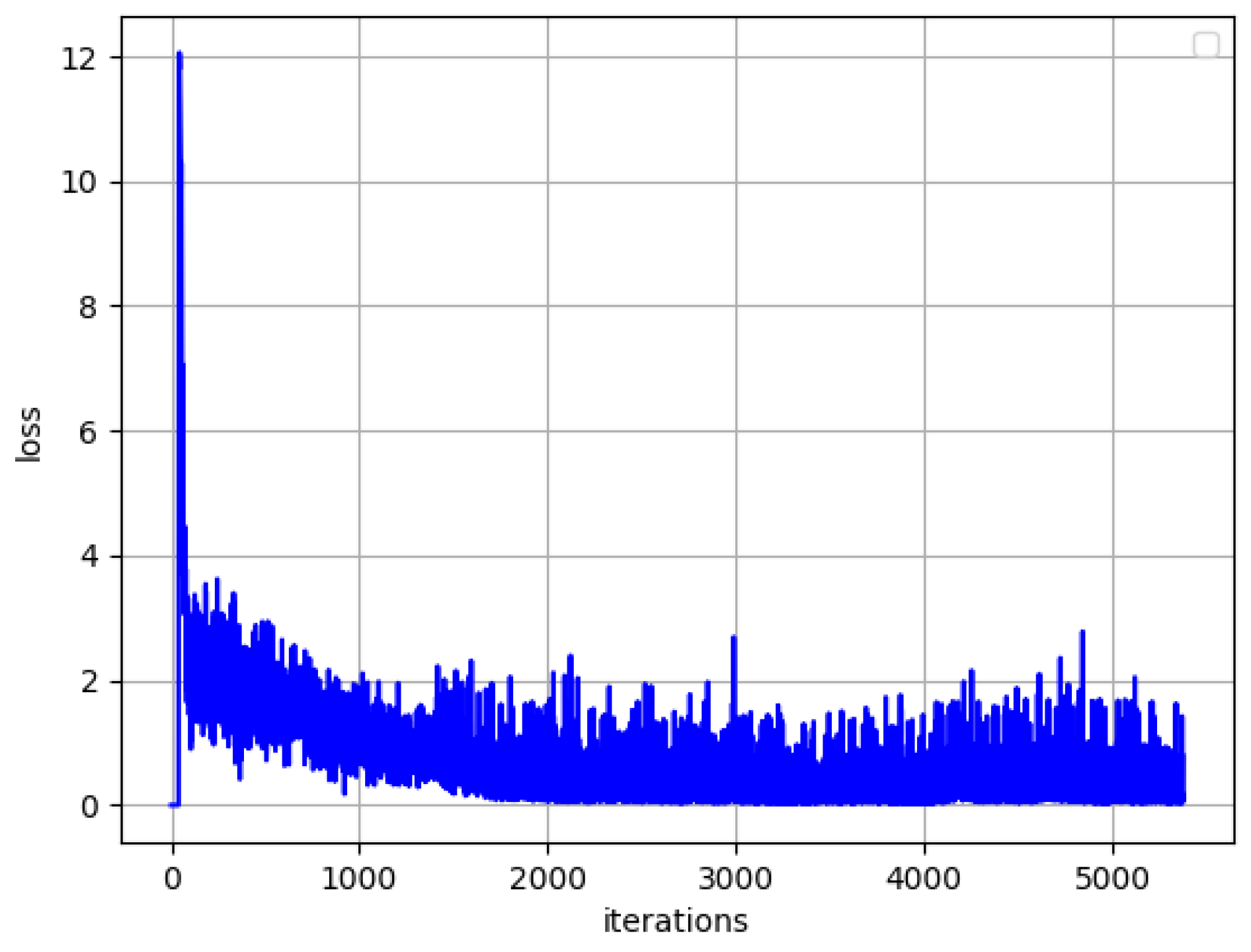
4.1. Experimental Results and Analysis

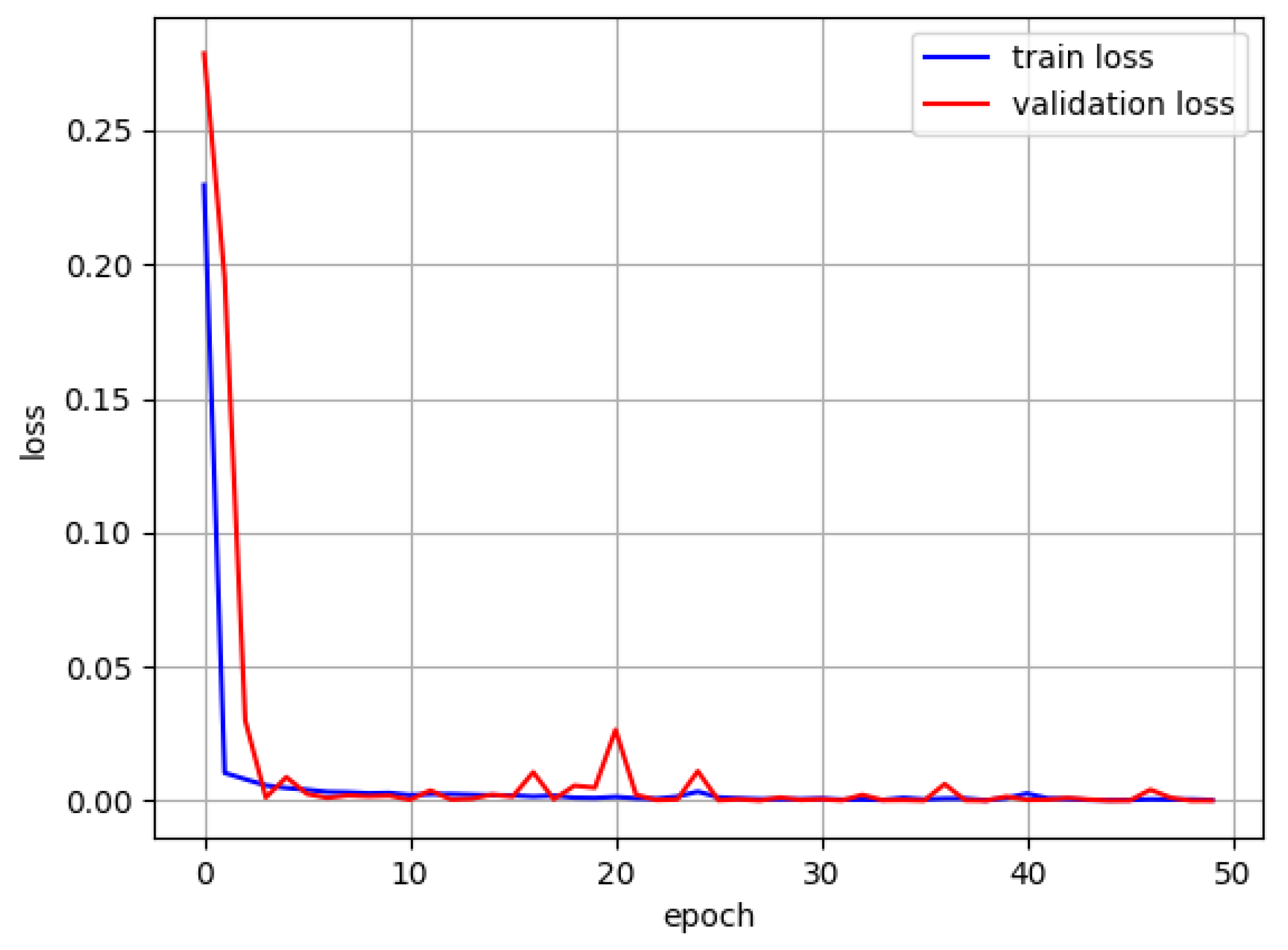
According to Section 2.2, we select $N=500$ and $n=200$. The loss value curve of the experimental results is shown in Figure 4.

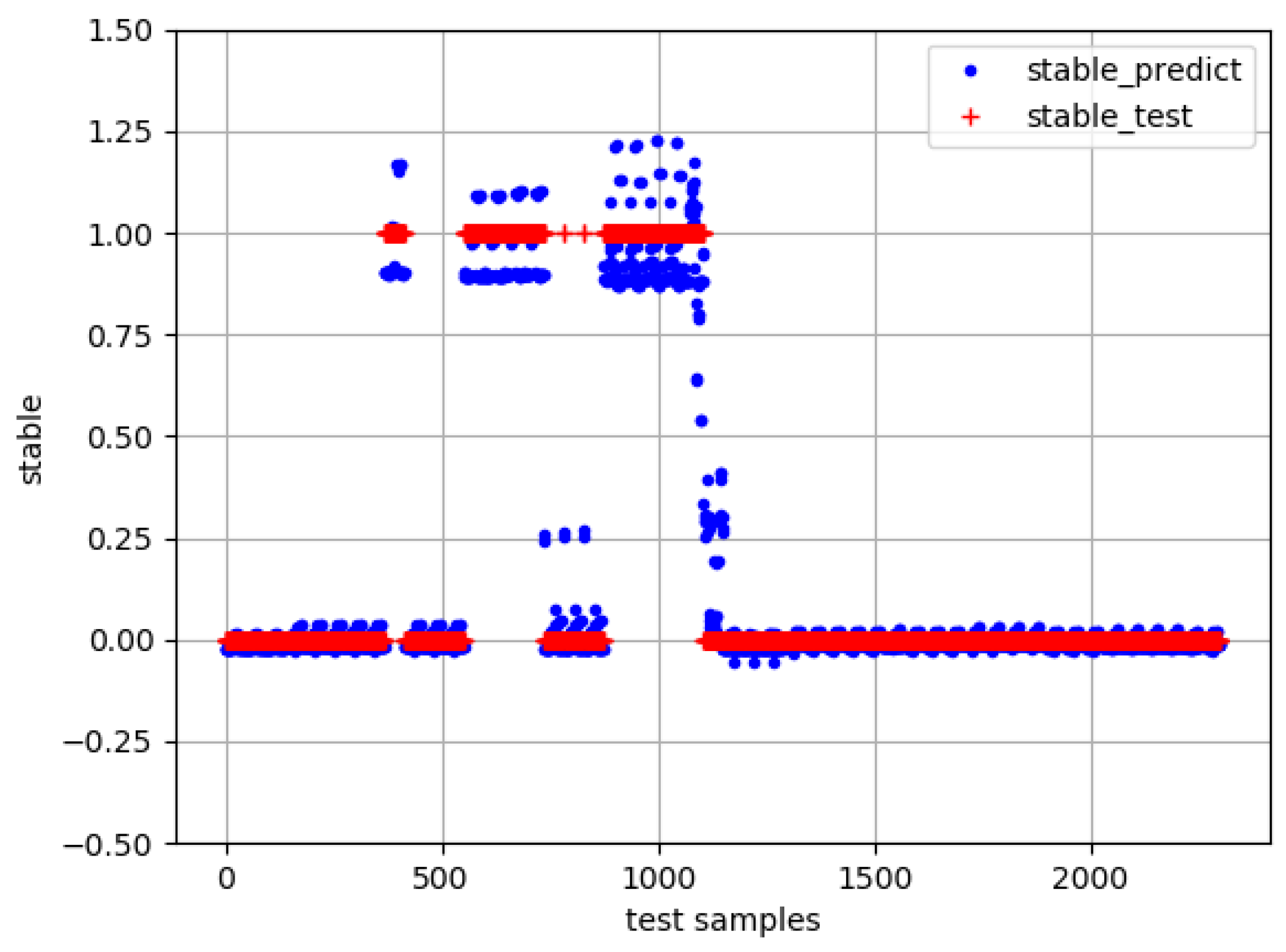
The results of the stability prediction on the test set are shown in Figure 5. Taking $0.5$ as the dividing line, the value that is greater than $0.5$ is classified as “1”, which is considered as stable. The value that is less than $0.5$ is classified as “0”, which is considered as unstable. The accuracy is $2294/2300$.

It is shown in

Table 2. Stability prediction results (first 200 cycles).

Predicted Value	Actual Value
	Stable	Unstable
Stable	462	0
Unstable	6	1832

that the false negative value is 6, i.e., six samples are actually stable. However, the prediction result is unstable. In order to maintain the stable operation of EI, it is acceptable to consider appropriate over-warning in real scenarios. While the false positive value is 0, i.e., the actual unstable sample is correctly predicted, which meets our requirements. In this paper, the threshold of accuracy is set to be 99%. The calculation is available with a precision of 1, a recall of 98.7%, and an f1-score of 99.4%.

The evaluation of stability prediction at this stage is to prepare for the decision optimization of subsequent reactive power compensation. In order to know in advance whether the EI would return to a stable state in the future, the characteristic time period is expected to be reduced. The data from the first 100 cycles would be intercepted, and the aforementioned CNN is still used for training. The accuracy is 2252/2300, which also meets the expected requirements.

The results of stability prediction are specifically analyzed in

Table 3. Stability prediction results (first 100 cycles).

Predicted Value	Actual Value
	Stable	Unstable
Stable	465	45
Unstable	3	1787

. Through calculating, the precision, the recall and the f1-score are 91.2%, 99.4% and 95.1%, respectively. The accuracy does not meet the requirement.

Although the precision of the prediction has achieved 97.9%, such rate is still relatively low and does not meet the requirement. Therefore, the structure of CNN is determined to be optimized. The parameters in the CNN is set to be fixed. The size of the convolution kernel is selected as $3\times 3$. The depth of the network is adjusted by changing the number of convolution layers. The number of feature extractions is altered by changing the number of convolution kernels per layer, which makes the extraction effect much better. After twenty experiments are conducted, the average value of the training results of different CNN structures with different parameters is obtained. The results are shown in

Table 4. Parameter settings of the convolutional neural network (CNN).

Number of Layers	Number of Convolution Kernels	Computation Time (s)	Precision (%)	Recall (%)	f1-Score (%)
4	64	3	91.2	99.4	95.1
4	128	6	95.3	87.4	91.2
4	256	15	95.0	97.9	96.4
6	64	4	99.5	89.3	94.1
6	128	7	95.0	98.3	96.6
6	256	19	98.6	93.4	96.0
8	64	4	94.0	80.8	86.9
8	128	8	94.3	84.4	89.1
8	256	21	94.8	93.6	94.2

.

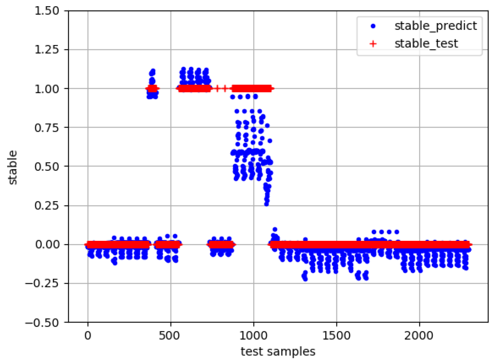
It can be seen from Table 4 that as the number of convolution kernels increases, the time for calculation increases substantially. The effect of increasing the number of the convolution layer on the calculation time is not obvious. The setting of the number of convolution layers and convolution kernels affects the prediction results. After twenty experiments are implemented, when the 6-layer convolution is set, and the number of convolution kernels per convolution layer is 64, the duration of calculation becomes shorter, and the accuracy is higher. The false positive value is smaller. More than half of the false positive values in the experimental results are all 0, which implies that the samples that are actually unstable are successfully predicted to be unstable. In this sense, the goal of stability prediction in this paper has been achieved. Thus, the model of CNN is selected. The results of the stability prediction on the test set are shown in Figure 6. The accuracy is 2236/2300, which meets the expected target.

The analysis of the stability prediction results is shown in

Table 5. Stability prediction results after optimization (first 100 cycles).

Predicted Value	Actual Value
	Stable	Unstable
Stable	404	0
Unstable	64	1832

. The false negative value is 64, i.e., 64 samples are actually stable. However, the prediction result is unstable, which is acceptable in the real engineering scenario. The false positive value is 0, i.e., the actual unstable samples are not predicted to be stable, which meets the expected requirements. Compared with the result before optimization, although the false negative value has increased, such value is reduced to be 0. In real-world applications, a false negative is acceptable, and a false positive is unacceptable. Therefore, the optimized results appear to meet the expected requirements. Through computation, the precision, the recall and the f1-score are 1, 86.3% and 92.7%, respectively.

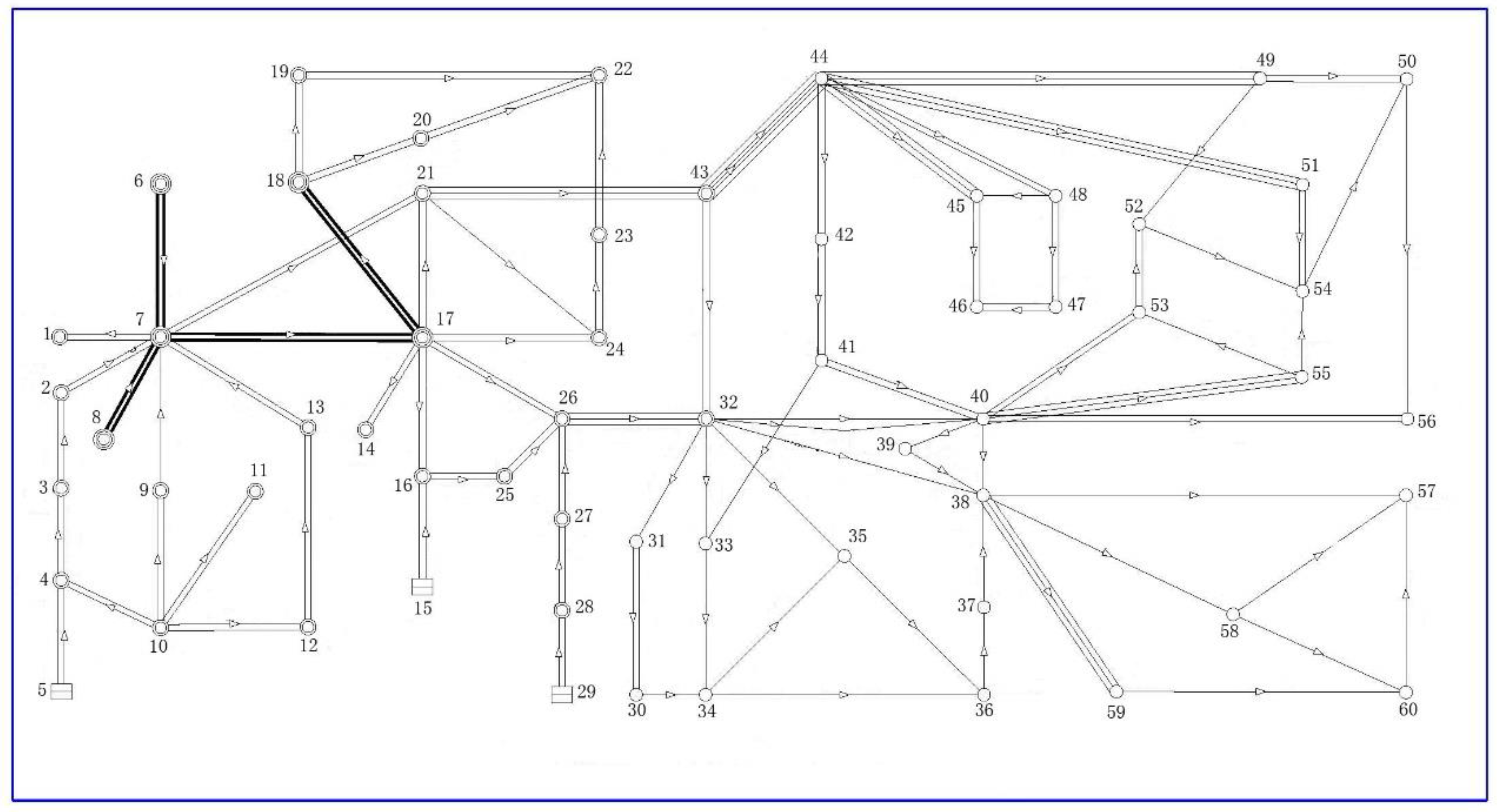
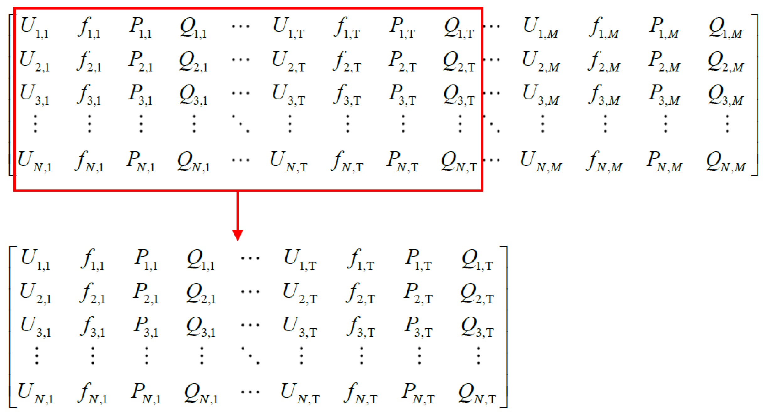
The output of existing research on stability prediction is mainly based on the analysis of single node data. Differently, this study selects the data of each node of the whole network as input data. Meanwhile, the data format is different. In order to verify the feasibility and effectiveness of the study as a comparative experiment, the SVM algorithm [16] is used for training. The false negative value is 141, i.e., 141 samples are stable. However, the prediction result is unstable, which is acceptable. The false positive value is 25, i.e., 25 samples are unstable but these samples are predicted to be stable. In real engineering practice, important information about voltage instability would be missed in such results. The future unstable states are difficult to be predicted accurately. Therefore, it is difficult to make a judgement, which is unacceptable. The obtained precision, the recall and the f1-score are 92.9%, 69.9% and 79.7%, respectively, which are much lower than the result obtained by our algorithm.

In summary, when data for each node in the whole grid system is used as high-dimensional input feature data within a certain characteristic time period, feature extraction can be better performed by deep learning CNN than by the conventional machine learning algorithm. A satisfactory fitting effect is obtained, and the application result in transient voltage stability judgment of EI achieves the expected target. Based on the mainstream power simulation software, a data batch processing toolkit has been developed, which improves the efficiency of data processing.

4.2. Simulation Example of Reactive Power Decision Optimization

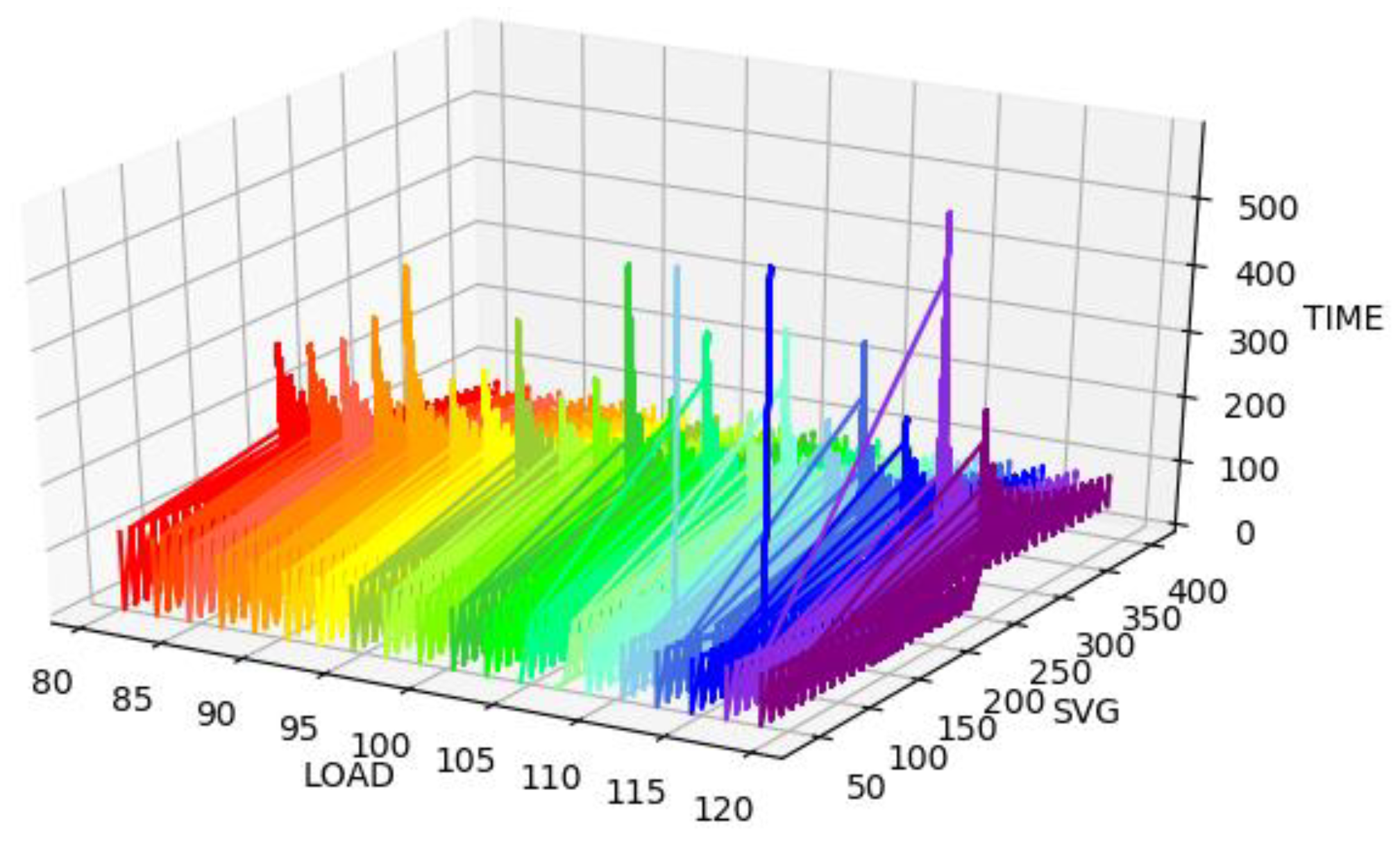
BPA is used to simulate different short-circuit faults. Since only the load model and load rate can be changed in BPA, the real-time load value cannot be collected. The system recovery time (cycle) corresponding to different load rates and the total SVG compensation is shown in Figure 7.

It can be seen that under the same load rate, as the amount of SVG compensation increases, the system fluctuates from an unstable state to a stable state, and the time of returning to the stable state decreases gradually.

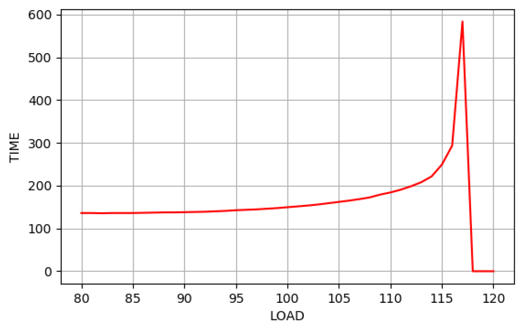
One set of SVG compensation was extracted. The load rate-time of returning to stable state (cycle) curve is drawn under the same SVG compensation. As is shown in Figure 8, with the increase in the load rate, the time of returning to a stable state increases gradually after the same SVG compensation is obtained until stability cannot be restored. In Figure 6, the system instability is represented by the time of returning to a stable state of $0$.

A numerical example is given in the following study where site A and site B represent for two cities. The load model is set as follows: (1) 30% constant resistance load, 40% constant current load and 30% constant power load at site A; and (2) 70% motor and 30% constant impedance with a load rate of 115% at site B. The short-circuit fault of single-circuit three-phase is set on buses with different voltage grades. Eight faults are considered in this example, including fault 1 (high-voltage level bus fault of 220 kV between site A and site B), fault 2 and fault 3 (220 kV high voltage grade bus fault on site B, i.e., the grid location studied in the experiment), as well as fault 4 to fault 8 (low voltage bus fault of 110 kV and 66 kV on site B).The fault clearing time is taken as 5 cycles, i.e., 0.1 s. Five SVGs are set at two 220 kV high voltage grade substations ($\mathrm{A}1$ substation and $\mathrm{A}2$ substation) and three 110 kV voltage grade substations ($\mathrm{A}3$ substation, $\mathrm{A}4$ substation and $\mathrm{A}5$ substation), respectively. The compensation values of five SVGs, which are intervals of the action in the proposed algorithm, are set as follows: [20 Mvar, 80 Mvar], [50 Mvar, 80 Mvar], [60 Mvar, 80 Mvar], [50 Mvar, 80 Mvar] and [50 Mvar, 80 Mvar]. In the proposed algorithm, the action space is discretized, and the discretized step is 10 Mvar. By this means, 1344 discrete actions are obtained. These actions are numbered from 1 to 1344. These actions are further converted into $one-hot$ form. The network is trained by CNN. The loss value is shown in Figure 9.

The optimization results based on deep reinforcement learning are shown in

Table 6. Decision Optimization Results.

Training Times	Number of Output Action
5000	34, 34, 34, 34, 34, 34, 34, 34
10,000	105, 105, 105, 105, 105, 105, 105, 105
15,000	389, 389, 389, 389, 389, 389, 389, 389
20,000	201, 201, 201, 241, 241, 241, 241, 241
25,000	19, 19, 19, 241, 241, 241, 241, 241

. The compensations value of each action in Table 5 for five SVGs are listed in

Table 7. Compensation Values.

Action	Compensation Value (Mvar)
19	20, 50, 70, 50, 70
34	20, 50, 80, 50, 60
105	20, 70, 60, 70, 50
201	30, 50, 60, 70, 50
241	30, 60, 60, 50, 50
389	40, 50, 60, 60, 50

. These two tables can be understood as follows. Taking the number in the first row of Table 6 as an example, when the network training times are 5000, the output action numbers of fault 1 to fault 8 are 34. According to the second line of Table 7, action 34 compensates for five SVGs with 20 Mvar, 50 Mvar, 80 Mvar, 50 Mvar and 60 Mvar, respectively.

Fault 1, fault 2 and fault 3 are in the high voltage bus. Thus, reactive compensation should be increased. It can be seen that at the initial stage of training, the differences from fault 1 to fault 3 and from fault 4 to fault 8 are not successfully identified. Similar action outputs with high compensation are given. However, the decision of reactive compensation for different grades could be given by increasing the training times. The difference can be seen in the results of later training.

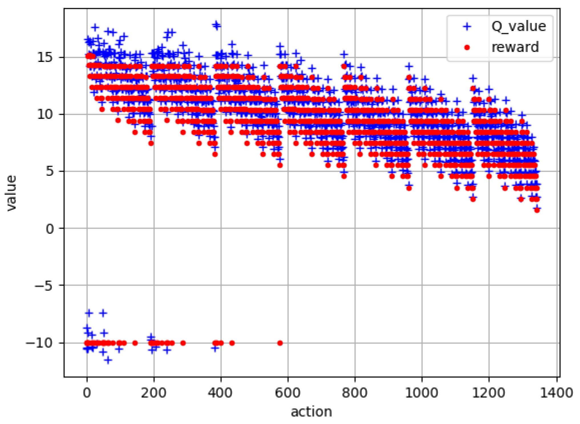
The contrast curve of $Q$ value and reward value are shown in Figure 10. It can be seen that the general trend of the $Q$ value is consistent with the general trend of the reward value. As the training time increases, the $Q$ value is constantly close to the reward value, which achieves the goal of training.

All buses with high voltage are set to be stable. The total compensation of SVG is the lowest. The decision scheme of the final test is shown in Table 6.

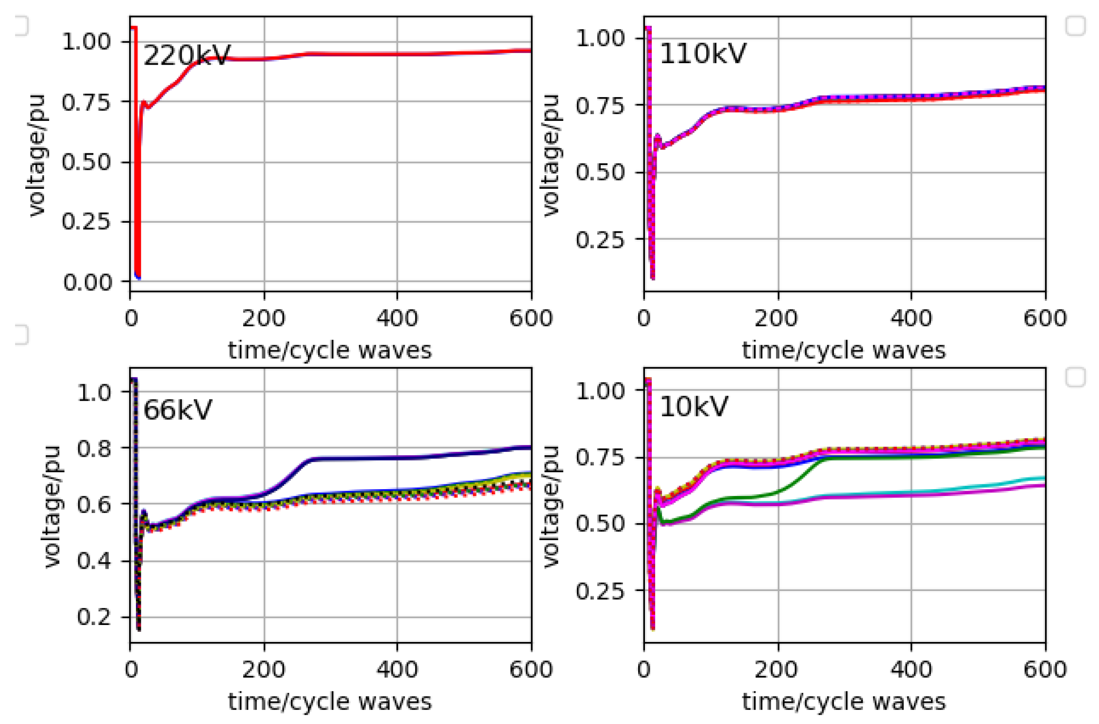
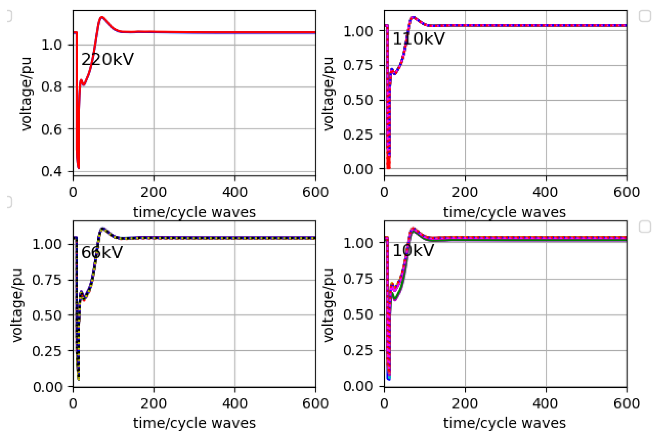
Fault 1 occurs on the highest level of the transmission bus between site A and site B. One of the decision schemes obtained by the model is action 19, i.e., five SVGs compensate 20 Mvar, 50 Mvar, 70 Mvar, 50 Mvar and 70 Mvar, respectively. It can be seen that the SVGs are distributed. The compensation value of each SVG is smaller than that of only two SVGs. The desired distributed setting of the reactive power compensation device is achieved. The stability result is shown in Figure 11. The time of returning to a stable state is about 550 cycles.

Fault 2 occurs on the high-voltage bus with 220 kV at site B. One of the decision schemes given by the model is action 34, that is, five SVGs compensate 20 Mvar, 50 Mvar, 80 Mvar, 50 Mvar and 60 Mvar, respectively. The stability result is shown in Figure 12. The time of returning to a state of stability is about 250 cycles.

Fault 3 occurs on the high-voltage bus with 220 kV at site B. One of the decision schemes given by the model is action 389, i.e., five SVGs compensate 40 Mvar, 50 Mvar, 60 Mvar, 60 Mvar and 50 Mvar, respectively. The time of returning to a stable state is about 295 cycles.

Fault 4 occurs on the high-voltage bus with 220 kV at site B. One of the decision schemes given by the model is action 34, i.e., five SVGs compensate 20 Mvar, 50 Mvar, 80 Mvar, 50 Mvar and 60 Mvar, respectively. The time of returning to the state of stability is about 50 cycles.

From the above analysis, the difference between the high voltage bus with 220 kV and 110 kV in the initial stage of training is not distinguished by the model. The scheme with the same total compensation amount is selected. Although the requirement of restoring stability can be met, the whole EI is subject to the impact of smaller short-circuit faulting with lower bus voltage level. In the later stage of training, a scheme for fault 4 to fault 8 is given by the model. Five SVGs compensate 30 Mvar, 60 Mvar, 60 Mvar, 50 Mvar and 50 Mvar, respectively. At this point, the total compensation amount is 250 Mvar. Fault 4 is set, and then action 241 is executed. The stability result is shown in Figure 13. The time of returning to a stable state is about 60 cycles. A better optimal decision scheme can be given by the model though training.

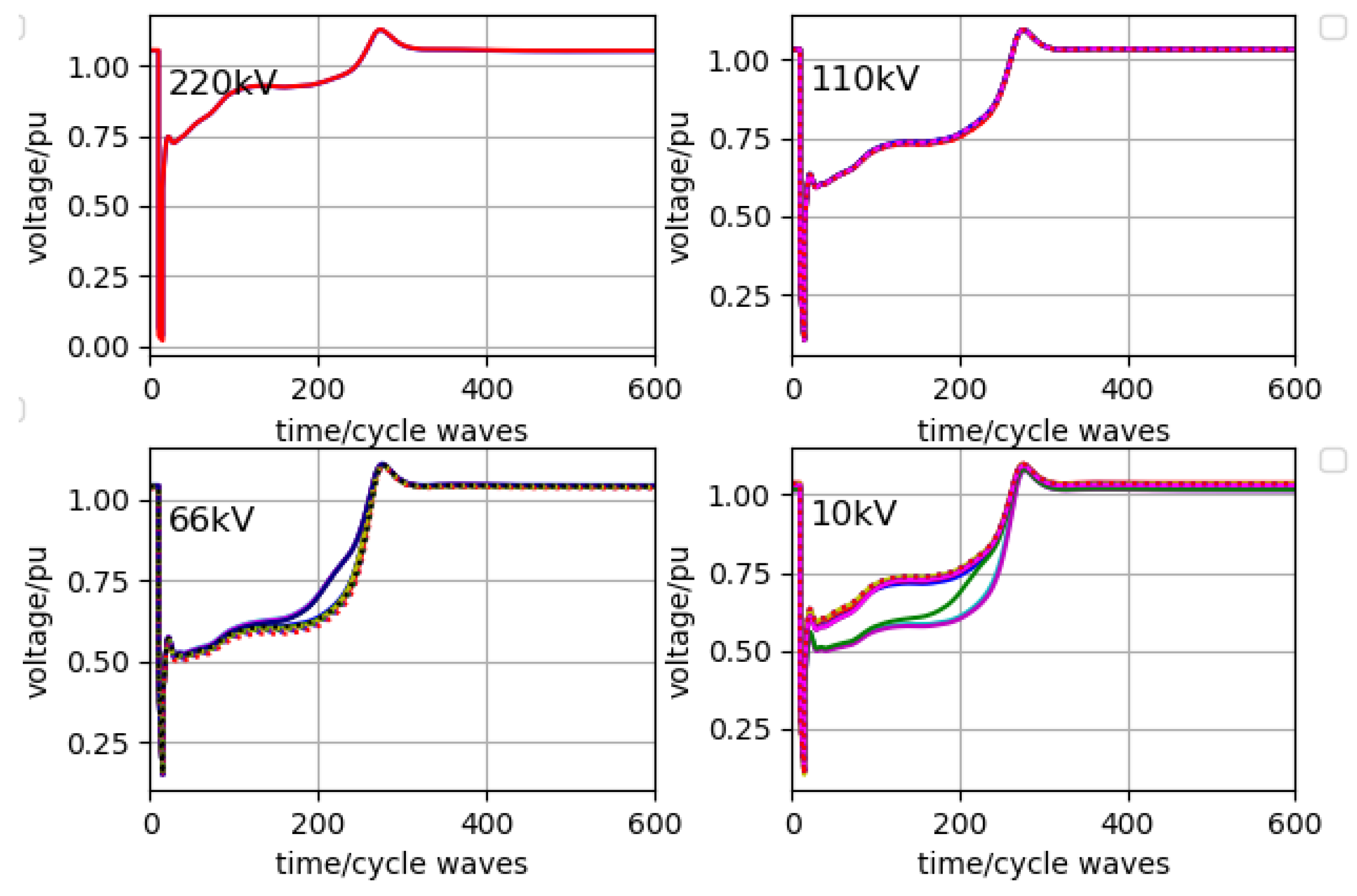
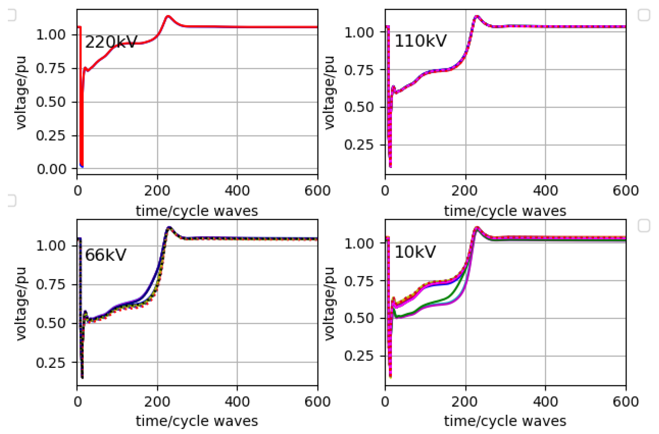
However, in the previous setting of the reward value calculation formula, only the requirement that buses with high voltage grade finally restore stability is considered. The time of returning to a stable state is not considered. Thereby, we can see from Figure 11 that although the strategy given by the algorithm ultimately achieves system stability, it is time consuming. The stable operation of the grid and the usage of the customer side’s load would also be affected. The calculation of rewards is changed by the choice. The time of returning to the stable state is taken into account. New and different strategies are given by the algorithm in the final experimental results. One of these strategies is action 673, i.e., five SVGs compensate 50 Mvar, 70 Mvar, 60 Mvar, 50 Mvar and 50 Mvar, respectively. Although the total compensation is slightly higher than the previous strategy, it can be seen that the compensation of each SVG is distributed more evenly.

Fault 1 is set, and action 673 is executed. The stable result is shown in Figure 14. When five SVGs compensate 50 Mvar, 70 Mvar, 60 Mvar, 50 Mvar and 50 Mvar, respectively, the time of returning to a stable state is about 200 cycles.

Based on the comparison of the above experimental results, it can be seen that the strategy proposed by the final algorithm meets the requirement of bus voltage stability. Meanwhile, the SVG presents distributed settings, and the output compensation is distributed uniformly. In addition, the distributed SVG conducts reactive compensation with a shorter timeframe, which greatly improves the efficiency of decision-making compared with conventional manual operations. The distributed SVG obtains stability within 200 cycles, which meets the requirement for secure and stable operation of the EI.

5. Conclusions

Based on EI architecture, this study proposes a decision optimization algorithm based on state judgment, in order to realize efficient, safe and stable operation of the EI. The experimental results show that the deep CNN is superior to the conventional machine learning algorithms with regards to feature extraction and prediction accuracy. In addition, a data batch processing toolkit based on BPA is developed to realize semi-automatic data batch processing, which improves the efficiency of data processing. Based on the stable state judgment, a deep reinforcement learning algorithm is proposed to optimize the reactive power compensation decision of EI. The experimental results not only show that this algorithm can achieve the system stability target, but can also fulfils the expectation of distributed reactive compensation and minimization of total reactive compensation.

Currently, a large number of simulation data can be generated off-line for training. The simulation and state feedback of continuous action changes cannot be realized. The action has to be discretized. In the future, it is necessary to realize the direct interface between simulation software and the deep learning platform, such that real-time simulation can be performed, and deep reinforcement learning algorithm can be used for continuous action learning and training.