Least Mean Squares and Recursive Least Squares Algorithms for Total Harmonic Distortion Reduction Using Shunt Active Power Filter Control

Abstract

This paper deals with the use of least mean squares (LMS, NLMS) and recursive least squares (RLS) algorithms for total harmonic distortion (THD) reduction using shunt active power filter (SAPF) control. The article presents a pilot study necessary for the construction of our own controlled adaptive modular inverter. The objective of the study is to find an optimal algorithm for the implementation. The introduction contains a survey of the literature and summarizes contemporary methods. According to this research, only adaptive filtration fulfills our requirements (adaptability, real-time processing, etc.). The primary benefit of the paper is the study of the efficiency of two basic approaches to adaptation ((N)LMS and RLS) in the application area of SAPF control. The study examines the impact of parameter settings (filter length, convergence constant, forgetting factor) on THD, signal-to-noise ratio (SNR), root mean square error (RMSE), percentage root mean square difference (PRD), speed, and stability. The experiments are realized with real current and voltage recordings (consumer electronics such as PC source without power factor correction (PFC), HI-FI amplifier, etc.), which contain fast dynamic transient phenomena. The realized model takes into account a delay caused by digital signal processing (DSP) (the implementation of algorithms on field programmable gate array (FPGA), approximately 1–5 μs) and a delay caused by the reaction time of the proper inverter (approximately 100 μs). The pilot study clearly showed that the RLS algorithm is the most suitable for the implementation of an adaptive modular inverter because it achieved the best results for all analyzed parameters.

1. Introduction

This paper deals with the topic of shunt active power filter (SAPF) control [1,2,3,4]. The aim of the study is to present a review of the methods of SAPF control used in practice. SAPFs are specially controlled voltage or current inverters, and they have to contain a very powerful computing unit that is able to react to the presence of higher harmonics immediately and reliably compensate these higher harmonics and reactive powers in the network.

Contemporary industrial enterprises usually have several types of electric equipment and loads, which can be separated into linear (heating, lamps, active loads, AC machine) and nonlinear (inverters, uninterruptible power supply (UPS) or LED lighting systems). Semiconductor inverters are the main source of negative effects on voltage quality in electricity distribution systems. These effects include the strain on the electric network from higher harmonics and reactive power.

Nowadays, two types of power filters are commonly used: passive [5] and active [6]. A passive power filter (PPF) consists of inductors and capacitors, and its circuit design is simple, but it has the following disadvantages [7]:

• An individual PPF is suitable only for a specific harmonic component since the harmonics are high or low enough to be eliminated. Designing a group of PPFs for various harmonics is uneconomical.
• Improving the power factor is less effective using a PPF, and in the case of change in the system architecture, the original design is not applicable.
• PPF implementation can lead to equipment damage due to the production of series of resonance parallel with the circuit impedance.
• The source impedance substantially affects PPF filtering properties.
• If a low-resistance circuit generates additional current harmonics, PPF becomes ineffective.
• The PPF takes more space.

Active filters can be classified as series active filters, shunt active filters, or a combination of these types. A series active filter solves problems related to voltage harmonics, such as voltage flicker, balancing, or sag. Conversely, a shunt active filter is used for solving current-related issues and reactive power compensation. For active power filter (APF) implementation, power switches, inductors, capacitors, and a control circuit are used. The control circuit calculates the compensation current necessary to prevent resonance by the elimination of current harmonics. The disadvantage of the APF is its greater switching loss than in the case of the passive filter. In addition, the complicated design of the APF controller results in low reliability. However, it is easy to develop microprocessors of power electronic components used in APF implementation, thanks to the modern level of technological advancement, so that these disadvantages can be overcome. The effectiveness of APFs is mainly influenced by determining the current harmonic, which can be obtained from either the frequency or time domain. The frequency domain calculation is based on Fourier analysis, and the time domain approach requires the use of instantaneous reactive power theory [7,8]. Using APFs, which are able not only to compensate harmonics but also improve the power factor and voltage regulation under different loads and unbalanced supply conditions, is the most effective solution. This fact has led researchers to develop and implement cost-effective control methods. Today, techniques such as instantaneous reactive power theory (d-q [9,10], p-q [11], modified d-q [12], p-q-r [13], vector [12]) are implemented to compensate current in the electrical grid [14].

The primary objective of the authors is to develop a controlled adaptive modular inverter, which will reflect the advantages of the adaptive systems. In the SAPF control area, these are new, still unused approaches. The adaptive systems are characterized by the ability to change their parameters according to information about the controlled system or processed signal. The real-time identification (adaptive) algorithm is the core of the adaptive system. Modern adaptive systems have already succeeded in many areas and industries (e.g., biological signal processing [15,16,17,18,19]; speech signal processing [20,21,22,23,24]; control and regulation area [25,26,27,28]; etc.), and current practice suggests that the same trend will continue in the future. For the practical use of these methods in real applications, theoretical and practical research of both new and current methods is needed. The application areas of these new approaches to digital signal processing are not very developed yet and are missing in some areas. This can also be said of the area of SAPF control. For this reason, there is a wide scope for further research and development. This paper presents a pilot study in this area.

The idea of adaptation is based on the properties of a living mass, so that we can talk about the so-called bio-inspired approach. It refers to inspiration from the ability of living organisms to adapt their behavior to changes in the environment, even though these changes are unfavorable. This phenomenon is called learning. Among systems that are capable of adaptation (learning), in addition to natural systems, we can now also include technical systems. Learning ability is sometimes considered as a definition of intelligence. It is natural that great effort is dedicated to equipping technical systems with this feature. Technical adaptive systems are characterized by the ability to adjust their parameters to current information about the controlled system or processed signal.

Currently, it is possible to observe a fast development of the methods of adaptive signal processing, e.g., various modifications of the basic adaptive algorithms with stochastic gradient [29,30,31] and recursive optimal adaptation [32,33,34], artificial neural networks [35,36], fuzzy systems [37,38], and their combination, known as fuzzy-neuro systems [38,39]. The area of adaptive signal processing is one of the fastest developing scientific/technical subjects. With the development of this area, there is often, and especially in technical practice, a question of how these new methods can be used to solve established goals in real applications. This paper focuses on the application of these methods in SAPF control.

In this study, currently used control methods for SAPF are analyzed in detail. The experimental part of the paper is focused primarily on adaptive methods for SAPF control. This progressive method of control has been increasingly applied over the last few years. Several basic approaches have evolved:

• Artificial intelligence techniques and soft computing techniques (adaptive neuro-fuzzy inference systems (ANFIS), adaptive linear neuron (ADALINE) ) [40,41,42,43,44,45]
• Adaptive algorithms (least mean squares (LMS) algorithm, normalized least mean squares (NLMS), recursive least mean squares (RLS) algorithm, etc.) [46,47,48].

This study deals with the implementation of LMS, NLMS, and RLS algorithms. The goal is to improve their behaviour for dynamically changing currents, where the nonlinear loads are quickly connected and disconnected. The experimental results are evaluated by total harmonic distortion (THD), signal-to-noise ratio (SNR), root mean square error (RMSE), and percentage root mean square difference (PRD).

2. Shunt Active Power Filter

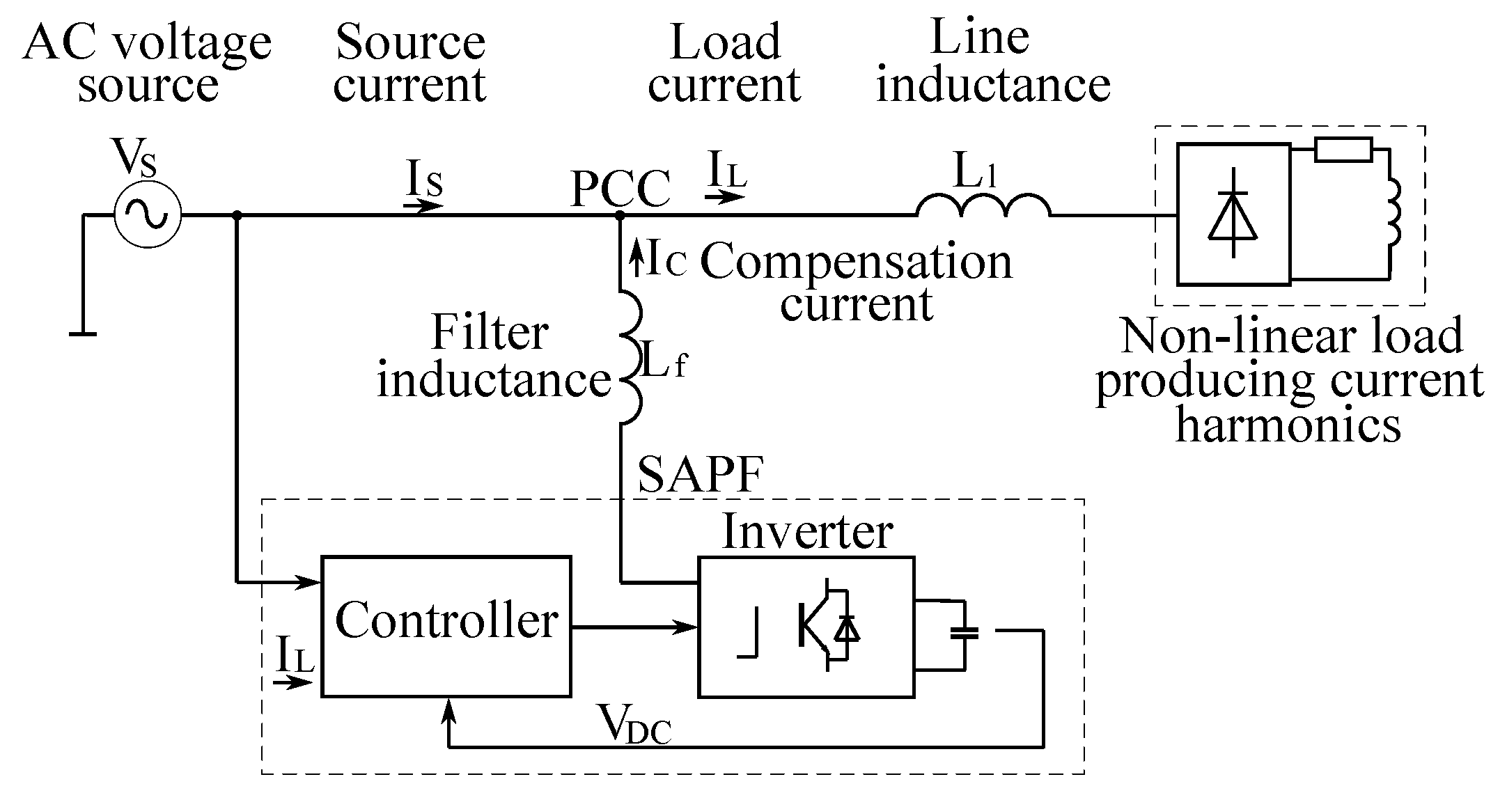
The parallel active filter forms the controlled current generator connected in parallel to a load. It can remove the unwanted higher harmonic components by generating the same components with the inverse phase and introducing them into the network. Thus, the current carried from the network is filtered and the deformations of the voltage, caused by non-sinusoidal voltage drops on power network impedance, are corrected. In this way, the compensation of the harmonic components can be carried out without the danger of unwanted resonance. Due to the generation of phase-shifted fundamental current harmonics, the filter is able to compensate the reactive power very quickly, eventually altering the asymmetric load to a symmetric one. The parallel filter is connected to the network via a coupling passive filter since the inverter of the active filter itself is the source of higher harmonics. The passive filter is a low-pass LC filter [6].

The current or voltage generator can consist of a bridge connection of semiconductor switches (insulated gate bipolar transistor (IGBT)). This generator in the three-phase system contains six switches and the current or voltage source. In practice, a solution with a voltage-source variant was proved. The desired shape of the current flowing to the filter can be obtained by the appropriate switching of transistors on the bridge. Figure 1 shows a simplified block diagram of a SAPF [6].

3. Control Methods for SAPF

Nowadays, SAPF control algorithms can be divided into two basic types of control: control in the time domain [1,49,50] and control in the frequency domain [49,51]. The control can be used both for one-phase [52] and three-phase connections [49,50,53] of SAPFs.

The control methods in the time domain can be separated according to a calculation of the compensation quantities (voltages or currents) using techniques working with the instantaneous powers in the power grid: p-q, unity power factor (UPF), perfect harmonic cancellation (PHC), and the synchronous detection method (SDM), or with the components of the instantaneous current values: synchronous reference frame (SRF), Id-Iq [49].

The control algorithm in the frequency domain uses a Fourier analysis, such as discrete Fourier transform (DFT), fast Fourier transform (FFT), or recursive discrete Fourier transform (RDFT), to obtain the reference values. This has the disadvantage of a long computing time and the generation of a time delay. One period of the signal is needed for the computation of FFT. Some publications compute FFT only from a half or a quarter of a period. This is suitable when the signal shape is symmetric over these stages [49].

3.1. Control in the Time Domain

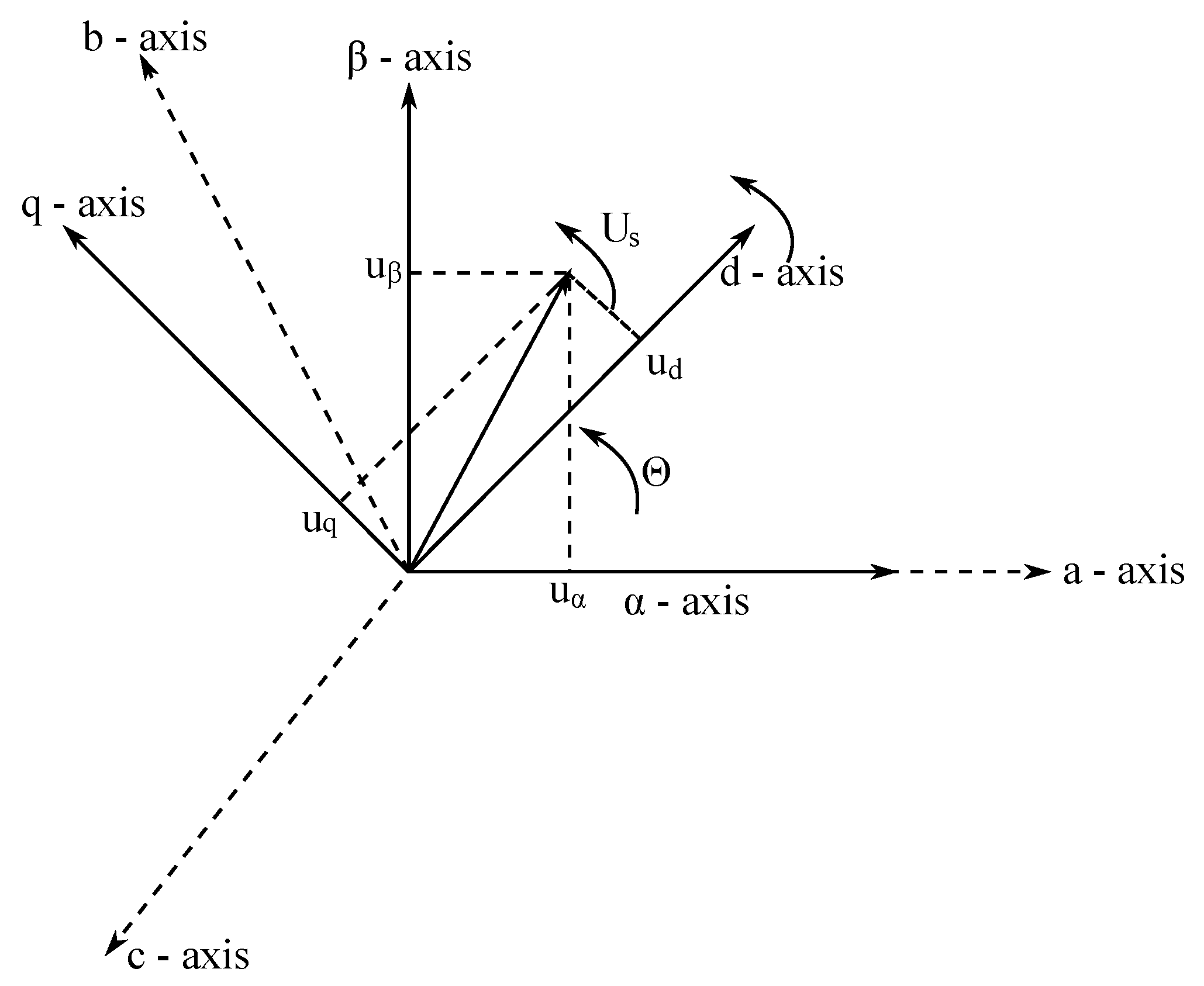
Methods using an instant value of the current or powers of the load are often used for this purpose. Some techniques employ suitable algebraic transformations (Clarke transform [9], transformation 3/2). The axis coordinates for these methods are shown in Figure 2.

3.2. Instantaneous Inactive Filter Control (p-q Theory)

The p-q method works with instant values in the three-wire or four-wire three-phase power system. It is suitable for the steady-state signals but also for a transition state. This theory is based on the Clarke transformation [9] of the three-phase voltages and currents in coordinates a-b-c into the coordinates $\alpha$-$\beta$-0, with a successive calculation of the instantaneous power components of p-q theory. After transformation, the following voltages and currents in coordinates $\alpha$-$\beta$-0 [11] are obtained:

$$\left[\begin{array}{c}{u}_0\\ u_{\alpha }\\ u_{\beta }\end{array}\right]=\sqrt{\frac{2}{3}}·\left[\begin{array}{ccc}\frac{1}{\sqrt{2}}& \frac{1}{\sqrt{2}}& \frac{1}{\sqrt{2}}\\ 1& -\frac{1}{2}& -\frac{1}{2}\\ 0& \frac{\sqrt{3}}{2}& -\frac{\sqrt{3}}{2}\end{array}\right]·\left[\begin{array}{c}{u}_{\mathrm{a}}\\ u_{\mathrm{b}}\\ u_{\mathrm{c}}\end{array}\right],$$

(1)

$$\left[\begin{array}{c}{i}_0\\ i_{\alpha }\\ i_{\beta }\end{array}\right]=\sqrt{\frac{2}{3}}·\left[\begin{array}{ccc}\frac{1}{\sqrt{2}}& \frac{1}{\sqrt{2}}& \frac{1}{\sqrt{2}}\\ 1& -\frac{1}{2}& -\frac{1}{2}\\ 0& \frac{\sqrt{3}}{2}& -\frac{\sqrt{3}}{2}\end{array}\right]·\left[\begin{array}{c}{i}_{\mathrm{a}}\\ i_{\mathrm{b}}\\ i_{\mathrm{c}}\end{array}\right].$$

(2)

$$p=u_{\alpha }·i_{\alpha }+u_{\beta }·i_{\beta }\mathrm{instantaneous}\mathrm{real}\mathrm{power}.$$

(3)

$$q=u_{\alpha }·i_{\beta }+u_{\beta }·i_{\alpha }\mathrm{instantaneous}\mathrm{imaginary}\mathrm{power}.$$

(4)

The power components p and q are related to the same $\alpha$-$\beta$ voltages and currents, and they can be written down together:

$$\left[\begin{array}{c}p\\ q\end{array}\right]=\left[\begin{array}{cc}{u}_{\alpha }& u_{\beta }\\ -u_{\beta }& -u_{\alpha }\end{array}\right]·\left[\begin{array}{c}{i}_{\alpha }\\ i_{\beta }\end{array}\right].$$

(5)

For detailed information, see [54,55].

3.3. Synchronous Reference Frame Method

Within the SRF method, the source currents ($i_{\mathrm{a}}$, $i_{\mathrm{b}}$, $i_{\mathrm{c}}$) are first detected and transformed into two-axis stationary coordinates $\alpha$-$\beta$-0 from the three-axis stationary coordinate a-b-c according to Equation (6) [10].

$$\left[\begin{array}{c}{i}_{\alpha }\\ i_{\beta }\\ i_0\end{array}\right]=\sqrt{\frac{2}{3}}·\left[\begin{array}{ccc}1& -\frac{1}{2}& -\frac{1}{2}\\ 0& \frac{\sqrt{3}}{2}& -\frac{\sqrt{3}}{2}\\ \frac{1}{\sqrt{2}}& \frac{1}{\sqrt{2}}& \frac{1}{\sqrt{2}}\end{array}\right]·\left[\begin{array}{c}{i}_{\mathrm{a}}\\ i_{\mathrm{b}}\\ i_{\mathrm{c}}\end{array}\right].$$

(6)

Two direct Park transformations [9] are used there. They enable the evaluation of the specific harmonic component of the input signals and low-pass filter. Next, the two-axis current quantities $i_{\alpha }$ and $i_{\beta }$ of the stationary axis $\alpha$-$\beta$ are transformed into a two-axis synchronous (rotating) coordinate d-q according to Equation (7), where cos$\Phi$ and sin$\Phi$ represent a synchronous unit of the vectors, which can be generated using a phase locked loop (PLL) [10].

$$\left[\begin{array}{c}{i}_{\mathrm{d}}\\ i_{\mathrm{q}}\end{array}\right]=\left[\begin{array}{cc}\cos \Phi & \sin \Phi \\ \sin \Phi & \cos \Phi \end{array}\right]·\left[\begin{array}{c}{i}_{\alpha }\\ i_{\beta }\end{array}\right].$$

(7)

The currents $i_{\mathrm{d}}$ and $i_{\mathrm{q}}$ contain both AC and DC components. The primary component of the current is the fixed DC part, and the AC component represents a harmonic part. This harmonic component can be easily extracted using the high-pass filter. The current $i_{\mathrm{d}}$ is the combination of the fundamental active current ($i_{\mathrm{d}\_\mathrm{DC}}$) and the harmonic current of the load ($i_{\mathrm{dh}}$). The primary component of the current rotates synchronously with the rotating axis, and it can be considered as the direct current. By the filtering of $i_{\mathrm{d}}$, the current representing the fundamental component of the current of the load in the synchronous axis is gained. Thus, the AC component $i_{\mathrm{dh}}$ can be obtained by subtracting $i_{\mathrm{d}\_\mathrm{DC}}$ from the total current $i_{\mathrm{d}}$, which leaves behind the harmonic component present in the current of the load. In the rotating axis, the current of axis q ($i_{\mathrm{q}}$) represents a sum of the fundamental reactive current and of the harmonic currents of the load. The current in axis q can be used for the calculation of the reference compensation current. The inverse transformation is made for the transformation of the currents from the two-axis synchronous axis d-q into a two-axis stationary axis $\alpha$-$\beta$ according to Equation (8) [10].

$$\left[\begin{array}{c}{i}_{\alpha }\\ i_{\beta }\end{array}\right]=\left[\begin{array}{cc}\cos \Phi & -\sin \Phi \\ \sin \Phi & \cos \Phi \end{array}\right]·\left[\begin{array}{c}{i}_{\mathrm{dh}}\\ i_{\mathrm{q}}\end{array}\right].$$

(8)

In the end, the current transformed from the two-axis stationary axis $\alpha$-$\beta$-0 back into the three-axis stationary axis a-b-c according to Equation (9) and the compensation reference currents $i_{\mathrm{ca}}^{*}$, $i_{\mathrm{cb}}^{*}$, and $i_{\mathrm{cc}}^{*}$ are obtained [10].

$$\left[\begin{array}{c}{i}_{\mathrm{ca}}^{*}\\ i_{\mathrm{cb}}^{*}\\ i_{\mathrm{cc}}^{*}\end{array}\right]=\sqrt{\frac{2}{3}}·\left[\begin{array}{ccc}1& 0& \frac{1}{\sqrt{2}}\\ -\frac{1}{2}& \frac{\sqrt{3}}{2}& \frac{1}{\sqrt{2}}\\ -\frac{1}{2}& -\frac{\sqrt{3}}{2}& \frac{1}{\sqrt{2}}\end{array}\right]·\left[\begin{array}{c}{i}_{\alpha }\\ i_{\beta }\\ i_0\end{array}\right].$$

(9)

3.4. Control of Instant Values of Current Components (ID-IQ Method)

This method uses the same system of coordinates as SRF, but unlike SRF, there is no need for a phase-locked loop (PLL) and synchronization. The currents $i_{\mathrm{d}}$ and $i_{\mathrm{q}}$ can be obtained from Equation (10) [50].

$$\left[\begin{array}{c}{i}_{\mathrm{d}}\\ i_{\mathrm{q}}\end{array}\right]=\sqrt{\frac{2}{3}}·\left[\begin{array}{ccc}\cos \Phi & \cos (\Phi -\frac{2\pi }{3})& \cos (\Phi -\frac{4\pi }{3})\\ -\sin \Phi & -\sin (\Phi -\frac{2\pi }{3})& -\sin (\Phi -\frac{4\pi }{3})\end{array}\right]·\left[\begin{array}{c}{i}_{\mathrm{a}}\\ i_{\mathrm{b}}\\ i_{\mathrm{c}}\end{array}\right],$$

(10)

where

$$cos\Phi =\frac{u_{\alpha }}{\sqrt{u_{\alpha }^2+u_{\beta }^2}},sin\Phi =\frac{u_{\beta }}{\sqrt{u_{\alpha }^2+u_{\beta }^2}},$$

(11)

where $u_{\alpha }$ and $u_{\beta }$ are from p-q theory. This method is also suitable for three-phase systems [50].

The conversion from coordinates d-q to coordinates a-b-c is the same as in the case of SRF. For detailed information see [56].

3.5. Control of Instantaneous Inactive Power in Coordinates p-q-r

This theory is characterized by a double transformation process: a first conversion of the voltages and currents from the coordinates a-b-c into coordinates $\alpha$-$\beta$-0 and a second conversion from the coordinates $\alpha$-$\beta$-0 to coordinates p-q-r according to the following equations [13]:

$$\left[\begin{array}{c}{i}_{\alpha }\\ i_{\beta }\\ i_0\end{array}\right]=\sqrt{\frac{2}{3}}·\left[\begin{array}{ccc}1& -\frac{1}{2}& -\frac{1}{2}\\ 0& \frac{\sqrt{3}}{2}& -\frac{\sqrt{3}}{2}\\ \frac{1}{\sqrt{2}}& \frac{1}{\sqrt{2}}& \frac{1}{\sqrt{2}}\end{array}\right]·\left[\begin{array}{c}{i}_{\mathrm{a}}\\ i_{\mathrm{b}}\\ i_{\mathrm{c}}\end{array}\right],$$

(12)

$$\left[\begin{array}{c}{u}_{\alpha }\\ u_{\beta }\\ u_{\beta }\end{array}\right]=\sqrt{\frac{2}{3}}·\left[\begin{array}{ccc}1& -\frac{1}{2}& -\frac{1}{2}\\ 0& \frac{\sqrt{3}}{2}& -\frac{\sqrt{3}}{2}\\ \frac{1}{\sqrt{2}}& \frac{1}{\sqrt{2}}& \frac{1}{\sqrt{2}}\end{array}\right]·\left[\begin{array}{c}{u}_{\mathrm{a}}\\ u_{\mathrm{b}}\\ u_{\mathrm{c}}\end{array}\right].$$

(13)

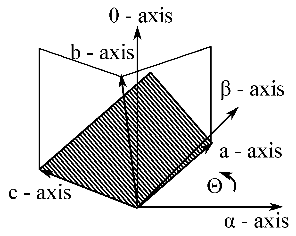
The physical importance of the coordinate transformation of the equations mentioned above is shown in Figure 3. The vertical angles from the plane $\alpha$-$\beta$ into coordinates a-b-c are the same, namely $\Phi =t{g}^{-1}(1/\sqrt{2})$, and axis a is located above axis $\alpha$ [13].

As shown in Figure 4a, the new coordinate ${\alpha }^{\prime }$-${\beta }^{\prime }$-0 is made by rotating axis 0 of the coordinate $\alpha$-$\beta$-0 using angle ${\Phi }_1$, which results in the alignment of axis $\alpha$ with a vector of the instantaneous spatial voltage ($e_{\alpha \beta }$) into the plane $\alpha$-$\beta$. The current of the spatial vector in coordinate ${\alpha }^{\prime }$-${\beta }^{\prime }$-0 can be expressed as [13]

$$\left[\begin{array}{c}{i}_{{\alpha }^{\prime }}\\ i_{{\beta }^{\prime }}\\ i_0\end{array}\right]=\left[\begin{array}{ccc}cos{\Phi }_1& sin{\Phi }_1& 0\\ -sin{\Phi }_1& cos{\Phi }_1& 0\\ 0& 0& 1\end{array}\right]·\left[\begin{array}{c}{i}_{\alpha }\\ i_{\beta }\\ i_0\end{array}\right]=\left[\begin{array}{ccc}\frac{e_{\alpha }}{e_{\alpha \beta }}& \frac{e_{\beta }}{e_{\alpha \beta }}& 0\\ -\frac{e_{\beta }}{e_{\alpha \beta }}& \frac{e_{\alpha }}{e_{\alpha \beta }}& 0\\ 0& 0& 1\end{array}\right]·\left[\begin{array}{c}{i}_{\alpha }\\ i_{\beta }\\ i_0\end{array}\right],$$

(14)

where

$$e_{\alpha \beta }=\sqrt{e_{\alpha }^2+e_{\beta }^2}.$$

(15)

Similarly, the coordinates p-q-r can occur by the rotation of axis ${\beta }^{\prime }$ of the coordinate ${\alpha }^{\prime }$-${\beta }^{\prime }$-0 using angle ${\Phi }_2$, as shown in Figure 4b. This results in the alignment of axis ${\alpha }^{\prime }$ with a vector of the instantaneous spatial voltage ($e_{\alpha \beta 0}$). The current of the spatial vector in the coordinate p-q-r is expressed as [13]

$$\left[\begin{array}{c}{i}_{\mathrm{p}}\\ i_{\mathrm{q}}\\ i_{\mathrm{r}}\end{array}\right]=\left[\begin{array}{ccc}cos{\Phi }_2& 0& sin{\Phi }_2\\ 0& 1& 0\\ -sin{\Phi }_2& 0& cos{\Phi }_2\end{array}\right]·\left[\begin{array}{c}{i}_{{\alpha }^{\prime }}\\ i_{{\beta }^{\prime }}\\ i_0\end{array}\right]=\left[\begin{array}{ccc}\frac{e_{\alpha }\beta }{e_{\alpha \beta 0}}& 0& \frac{e_0}{e_{\alpha \beta 0}}\\ 0& 1& 0\\ -\frac{e_0}{e_{\alpha \beta 0}}& 0& \frac{e_{\alpha }\beta }{e_{\alpha \beta 0}}\end{array}\right]·\left[\begin{array}{c}{i}_{{\alpha }^{\prime }}\\ i_{{\beta }^{\prime }}\\ i_0\end{array}\right],$$

(16)

where

$$e_{\alpha \beta 0}=\sqrt{e_{\alpha }^2+e_{\beta }^2+e_0^2}.$$

(17)

The axes ${\beta }^{\prime }$ and q are identical. By the combination of Equations (16) and (18), the transformation from coordinate $\alpha$-$\beta$-0 into coordinate p-q-r occurs [13]:

$$\left[\begin{array}{c}{i}_{\mathrm{p}}\\ i_{\mathrm{q}}\\ i_{\mathrm{r}}\end{array}\right]=\left[\begin{array}{ccc}\frac{e_{\alpha }}{e_{\alpha \beta 0}}& \frac{e_{\beta }}{e_{\alpha \beta 0}}& \frac{e_0}{e_{\alpha \beta 0}}\\ -\frac{e_{\beta }}{e_{\alpha \beta }}& \frac{e_{\alpha }}{e_{\alpha \beta }}& 0\\ -\frac{e_0·e_{\alpha }}{e_{\alpha \beta 0·e_{\alpha \beta }}}& -\frac{e_0·e_{\beta }}{e_{\alpha \beta 0·e_{\alpha \beta }}}& \frac{e_{\alpha \beta }}{e_{\alpha \beta 0}}\end{array}\right]·\left[\begin{array}{c}{i}_{\alpha }\\ i_{\beta }\\ i_0\end{array}\right].$$

(18)

3.6. Unity Power Factor

The UPF method requires that the load and active power filter are considered as a linear load.

If this is fulfilled, the source current after compensation is expressed as

$$i_{{\mathrm{s}}_{\mathrm{ref}}}=K·u_{\mathrm{s}},$$

(19)

where K according to Equation (20) is the conductivity of the nonlinear load and the power active filter. After compensation, the source current is sinusoidal with the same shape as the source voltage, and they are in phase. No higher harmonics are present in the current source, and the power factor is equal to one [1,52].

$$K=\frac{{\overrightarrow{p}}_{\mathrm{L}\alpha \beta }+{\overrightarrow{p}}_{\mathrm{L}0}}{{(u_0^2+u_{\alpha }^2+u_{\beta }^2)}_{\mathrm{DC}}}.$$

(20)

The power delivered by the source is

$$ps=u_{\mathrm{s}}·i_{{\mathrm{s}}_{\mathrm{ref}}}=u_{\mathrm{s}}·K·u_{\mathrm{s}}=K(u_0^2+u_{\alpha }^2+u_{\beta }^2).$$

(21)

The reference current of the source is defined as

$$\left[\begin{array}{c}{i}_{\mathrm{s}{0}_{\mathrm{ref}}}\\ i_{\mathrm{s}{\alpha }_{\mathrm{ref}}}\\ i_{\mathrm{s}{\beta }_{\mathrm{ref}}}\end{array}\right]=K·\left[\begin{array}{c}{u}_0\\ u_{\alpha }\\ u_{\beta }\end{array}\right]=\frac{{\overrightarrow{p}}_{\mathrm{L}\alpha \beta }+{\overrightarrow{p}}_{\mathrm{L}0}}{{(u_0^2+u_{\alpha }^2+u_{\beta }^2)}_{\mathrm{DC}}}·\left[\begin{array}{c}{u}_0\\ u_{\alpha }\\ u_{\beta }\end{array}\right].$$

(22)

3.7. Perfect Harmonic Cancellation

The result of these methods is the compensation of all of the harmonic currents and the fundamental reactive power taken by the load. The current of the source is in phase with a fundamental component of the voltage of the source at the point of common coupling (PCC) [1]. The reference source current is defined as

$$i_{{\mathrm{s}}_{\mathrm{ref}}}=K·u_1^{+},$$

(23)

where $u_1^{+}$ is the spatial vector of voltage with a fundamental harmonic of the source at the PCC.

The power delivered by the source is expressed as

$$ps=u_{\mathrm{s}}·i_{{\mathrm{s}}_{\mathrm{ref}}}=u_{\mathrm{s}}·K·u_1^{+}=K(u_{\alpha }·u_{\alpha 1}^{+}+u_{\beta }·u_{\beta 1}^{+}),$$

(24)

where

$$K=\frac{{\overrightarrow{p}}_{\mathrm{L}\alpha \beta }+{\overrightarrow{p}}_{\mathrm{L}0}}{u_{\alpha 1}^{+2}+u_{\beta 1}^{+2}}.$$

(25)

In the end, the reference current of the source is defined:

$$\left[\begin{array}{c}{i}_{\mathrm{s}{0}_{\mathrm{ref}}}\\ i_{\mathrm{s}{\alpha }_{\mathrm{ref}}}\\ i_{\mathrm{s}{\beta }_{\mathrm{ref}}}\end{array}\right]=K·\left[\begin{array}{c}0\\ u_{\alpha 1}\\ u_{\beta 1}\end{array}\right]=\frac{{\overrightarrow{p}}_{\mathrm{L}\alpha \beta }+{\overrightarrow{p}}_{\mathrm{L}0}}{u_{\alpha 1}^{+2}+u_{\beta 1}^{+2}}·\left[\begin{array}{c}0\\ u_{\alpha 1}^{+}\\ u_{\beta 1}^{+}\end{array}\right].$$

(26)

3.8. Synchronous Detection Method

This theory can work effectively in symmetric or asymmetric systems because the compensation currents are calculated by taking into account the voltages of individual phases. This theory is used to calculate the compensation currents, while the three-phase source powers a highly nonlinear load. The method of the uniform distribution of the SDM current is used in this study to compute three-phase compensation currents that are supplied by the active filter [53].

When calculating three-phase compensation currents using the method of equal distribution of SDM current, the following assumptions are taken into account: the voltage is not distorted and the loss in the neutral wire is negligible [53].

Assume that the maximal values of source currents are symmetric after compensation:

$$I_{\mathrm{am}}=I_{\mathrm{bm}}=I_{\mathrm{cm}}=I_{\mathrm{m}}.$$

(27)

The maximal values of the active curents in each phase after compensation are

$$I_{\mathrm{am}}=\frac{2P_{\mathrm{a}}}{U_{\mathrm{am}}},I_{\mathrm{bm}}=\frac{2P_{\mathrm{b}}}{U_{\mathrm{bm}}},I_{\mathrm{cm}}=\frac{2P_{\mathrm{c}}}{U_{\mathrm{cm}}},$$

(28)

where $P_{\mathrm{a}}$, $P_{\mathrm{b}}$, and $P_{\mathrm{c}}$ are the real powers of each phase, and $U_{\mathrm{am}}$, $U_{\mathrm{bm}}$, and $U_{\mathrm{cm}}$ are the maximal values of the voltages of each phase.

Overall average power is defined as

$$P_{\mathrm{Tav}}=P_{\mathrm{a}}+P_{\mathrm{b}}+P_{\mathrm{c}}.$$

(29)

By adjusting, we get

$$U_{\mathrm{t}}=U_{\mathrm{am}}+U_{\mathrm{bm}}+U_{\mathrm{cm}},$$

(30)

$$P_{\mathrm{a}}=\frac{U_{\mathrm{am}}}{U_{\mathrm{t}}}{P}_{\mathrm{av}},P_{\mathrm{b}}=\frac{U_{\mathrm{bm}}}{U_{\mathrm{t}}}{P}_{\mathrm{av}},P_{\mathrm{c}}=\frac{U_{\mathrm{cm}}}{U_{\mathrm{t}}}{P}_{\mathrm{av}}.$$

(31)

The currents of the reference active source are calculated as

$$i_{\mathrm{ac}\mathrm{c}}\left(t\right)=\frac{2P_{\mathrm{av}}}{U_{\mathrm{am}}·U_{\mathrm{t}}}{u}_{\mathrm{an}}\left(t\right),$$

(32)

$$i_{\mathrm{bc}\mathrm{c}}\left(t\right)=\frac{2P_{\mathrm{av}}}{U_{\mathrm{bm}}·U_{\mathrm{t}}}{u}_{\mathrm{bn}}\left(t\right),$$

(33)

$$i_{\mathrm{cc}\mathrm{c}}\left(t\right)=\frac{2P_{\mathrm{av}}}{U_{\mathrm{cm}}·U_{\mathrm{t}}}{u}_{\mathrm{cn}}\left(t\right),$$

(34)

where the compensation currents are defined as

$$i_{\mathrm{c}\mathrm{an}}\left(t\right)=i_{\mathrm{an}}\left(t\right)-i_{\mathrm{ac}\mathrm{c}}\left(t\right),$$

(35)

$$i_{\mathrm{c}\mathrm{bn}}\left(t\right)=i_{\mathrm{bn}}\left(t\right)-i_{\mathrm{bc}\mathrm{c}}\left(t\right),$$

(36)

$$i_{\mathrm{c}\mathrm{cn}}\left(t\right)=i_{\mathrm{cn}}\left(t\right)-i_{\mathrm{cc}\mathrm{c}}\left(t\right).$$

(37)

3.9. Selection of the Optimal Method

Revuelta et al. [12] analyzed the strategies gained from five formulations of the instantaneous power theory (d-q [9,10], p-q [11], modified d-q [12], p-q-r [13], and vector [12]) applied on symmetrical, asymmetrical, and non-sinusoidal symmetrical nonlinear systems. They compare the performance of the compensation using two quantities measured in the source currents after compensation: the value of THD and the effective value of the current in the neutral wire in a three-phase four-wire system. The methods p-q, p-q-r, d-q, and vector obtained a zero current through the neutral wire, but the modified p-q methods did not obtain these results.

The vector and d-q methods only gained zero THD after compensation. The p-q and p-q-r techniques reached distortion below 10%. The modified p-q method exceeds this value in both cases.

The effective value of the current through the neutral wire is zero in the case of the symmetric system. Thus, when Equation (38) is valid,

$$I_1+I_2+I_3=0.$$

(38)

Since we work with a modular inverter that can work in both single-phase and three-phase systems, there is a requirement that an algorithm also works in both systems. Neither of the above-mentioned three-phase algorithms satisfies this requirement. Of course, there are different variants for single-phase systems, e.g., p-q theory [57,58], but this requires modification of the algorithm for each system. The next requirement is the real-time operating of the algorithms. Neither of the former methods met both conditions, which led us to the idea of using adaptive filtration, with which the authors have extensive experience in other areas. The advantage of the proposed concept is that the adaptive algorithms could effectively work in non-symmetric system, thus a zero current could be reached in the neutral wire. Its next benefit is the possibility of optimal settings of the adaptive filters for the individual phases. It can be expected that these settings will be different for each phase, resulting in better results than in the case of existing methods.

4. Adaptive Filtration

Adaptive filters are in practice used in an unknown environment, where the preliminary identification is challenging, or in a time-variant environment, which is unpredictable. In these cases, the digital finite impulse response (FIR) or infinite impulse response (IIR) filters with adaptive coefficients, which vary in time, are used. These filters are named adaptive filters [59,60,61,62,63].

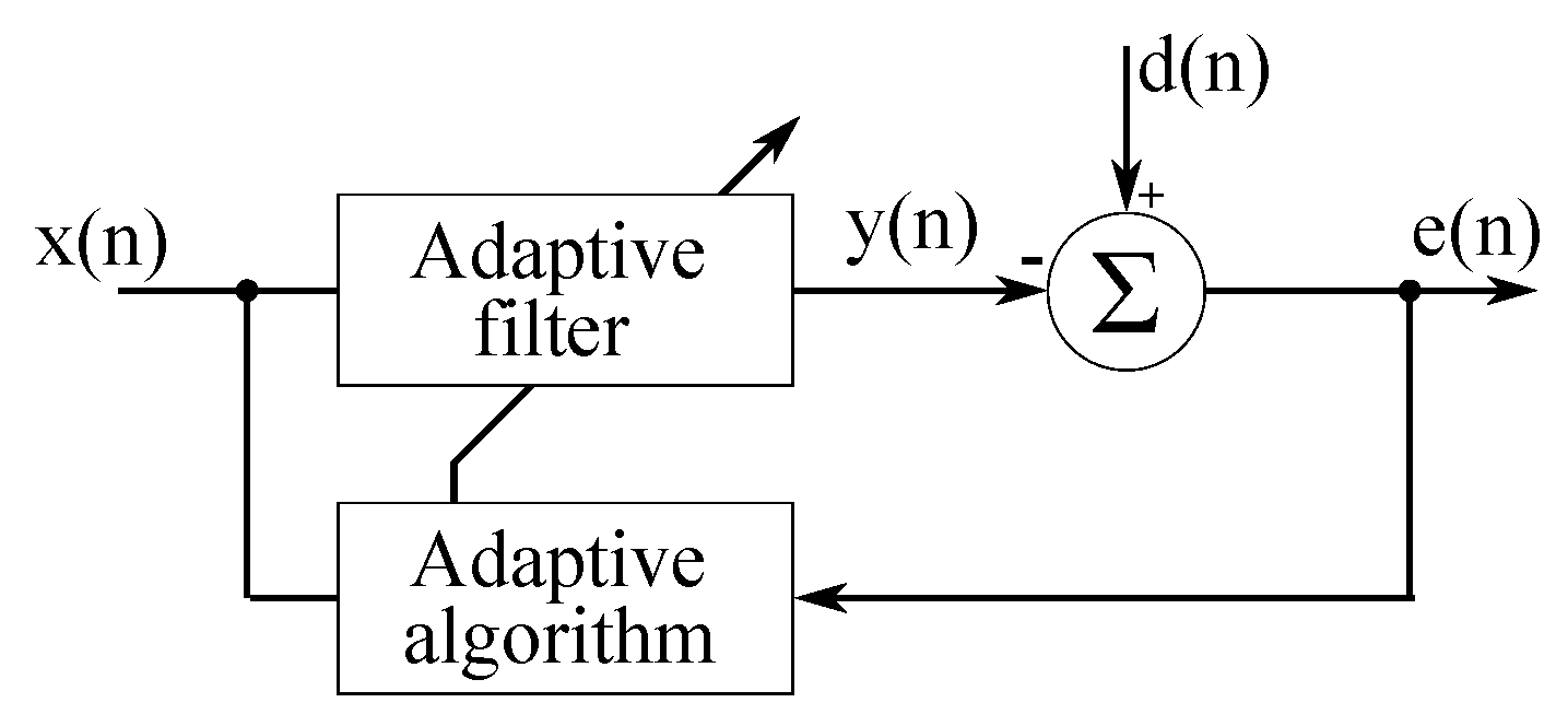
Figure 5 shows the general structure of an adaptive filter, where n is the number of iterations, $x\left(n\right)$ is the reference signal, $d\left(n\right)$ is the input signal, $e\left(n\right)$ is the output error signal, and $y\left(n\right)$ is the output desired signal. The error signal $e\left(n\right)$ is defined as $e\left(n\right)=d\left(n\right)-y\left(n\right)$ and is used to create a purpose function $\xi \left(n\right)$, which is needed in the adaptive algorithm to determine the appropriate optimal adaptive filter coefficient. The result of the process is the gradual reduction of the purpose function value to its minimum [59].

The purpose function for the LMS algorithm is defined as

$$\xi \left(n\right)=E\left[e^2\left(n\right)\right]=E\left[{(d\left(n\right)-y\left(n\right))}^2\right],$$

(39)

and the purpose function for the RLS algorithm is expressed as

$$\genfrac{}{}{0pt}{}{\xi \left(n\right)={\displaystyle \sum _{\mathrm{k}=1}^{\mathrm{n}}}{p}_{\mathrm{n}}\left(k\right)e_{\mathrm{n}}^2\left(k\right),}{p_{\mathrm{n}}\left(k\right)={\lambda }^{\mathrm{n}-\mathrm{k}},}$$

(40)

where $k=1,2,3,\dots n$ and parameter $\lambda$ is denoted as a factor for forgetting in the range of 0 to 1, but it is recommended to use values ranging from 0.95 to 1.

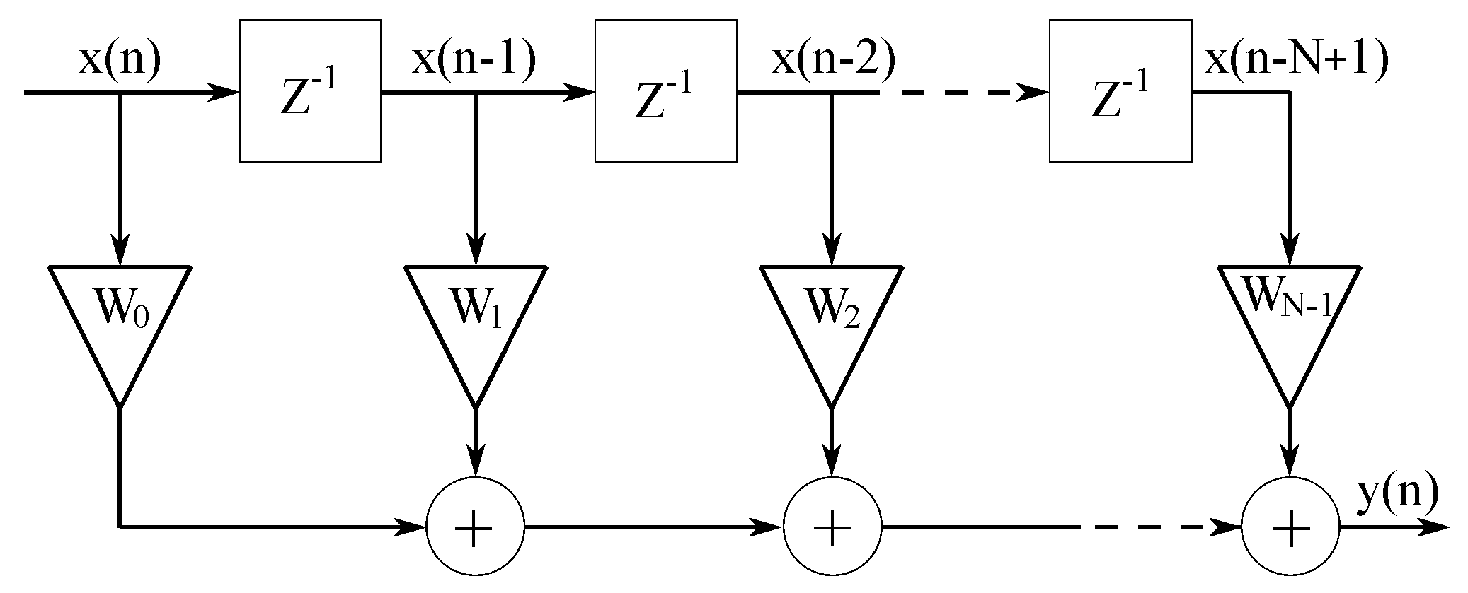
The block diagram of the adaptive filter is shown in Figure 6, where $w_{\mathrm{i}}$ represents the coefficients of the scale vector of the transversal FIR filter and $Z^{-1}$ represents the delay. This block diagram is valid both for LMS and RLS algorithms. In this study, the input signal is in the form of a column vector defined by the following equation:

$$\overrightarrow{x}\left(n\right)={[x\left(n\right)x(n-1)x(n-2)\dots x(n-N+1)]}^{\mathrm{T}}.$$

(41)

The scale vector of the transversal filter is

$$\overrightarrow{w}\left(n\right)={[w_0\left(n\right)w_1\left(n\right)w_2\left(n\right)\dots w_{\mathrm{N}-1}\left(n\right)]}^{\mathrm{T}}.$$

(42)

The output signal of the adaptive filter is expressed as

$$y\left(n\right)={\displaystyle \sum _{\mathrm{i}=0}^{\mathrm{N}-1}}{w}_{\mathrm{i}}\left(n\right)x(n-i).$$

(43)

More information about the adaptive filtration is provided in [62,63,64,65,66,67]. The algorithms used in this study are further described from the point of view of proper implementation. In [68,69,70,71], the algorithms are explained in detail. It is essential to state that all algorithms were implemented based on virtual instrumentation in the LabVIEW development environment [72,73,74].

4.1. Least Mean Squares Algorithm

The LMS algorithm is the main performer in the class of stochastic gradient algorithms based on the theory of Wiener filtration, stochastic averaging, and the least squares method [48].

Each iteration of the LMS algorithm requires three different steps, in this order:

• Filter output $y\left(n\right)$ is calculated according to Equation (43).
• The value of the estimated error is calculated as $e\left(n\right)=d\left(n\right)-y\left(n\right)$.
• The weights of the filter vector are updated according Equation (44) [48].

  $$\overrightarrow{w}(n+1)=\overrightarrow{w}\left(n\right)+2\mu e\left(n\right)\overrightarrow{x}\left(n\right).$$

  (44)

The parameter $\mu$ is called the convergence constant or the step size of the LMS algorithm. It is a low positive constant that influences the properties of algorithm adaptation (the speed of convergence, filter stability, etc.) [48].

4.2. Normalized Least Mean Squares Algorithm

If the input signal $x\left(n\right)$ gets relatively high values, the use of the LMS algorithm results in amplification of the noise. The normalized LMS (NLMS) algorithm employs a variable convergence constant for each iteration, which is calculated using the input signal power [75,76,77].

$$\overrightarrow{w}(n+1)=\overrightarrow{w}\left(n\right)+\frac{\mu }{\parallel \overrightarrow{x}\left(n\right)\parallel }\overrightarrow{x}\left(n\right)e\left(n\right),$$

(45)

where

$$\mu \left(n\right)=\frac{\mu }{\parallel \overrightarrow{x}{\left(n\right)\parallel }^2}.$$

(46)

4.3. Discussion of the Choice of Coefficient $\mu$ Value

A quantity $\mu$ represents a step size. This constant has a significant influence on the speed and stability of the adaptive algorithm convergence. Substitution of the correct value (typically a small positive constant) for $\mu$ is necessary for the proper operation of the LMS algorithm:

• If the selected value of $\mu$ is too small, the time required to find the optimal solution by an adaptive filter is too long.
• If the chosen value of $\mu$ is too high, the adaptive filter becomes unstable, and the output brings deviations.

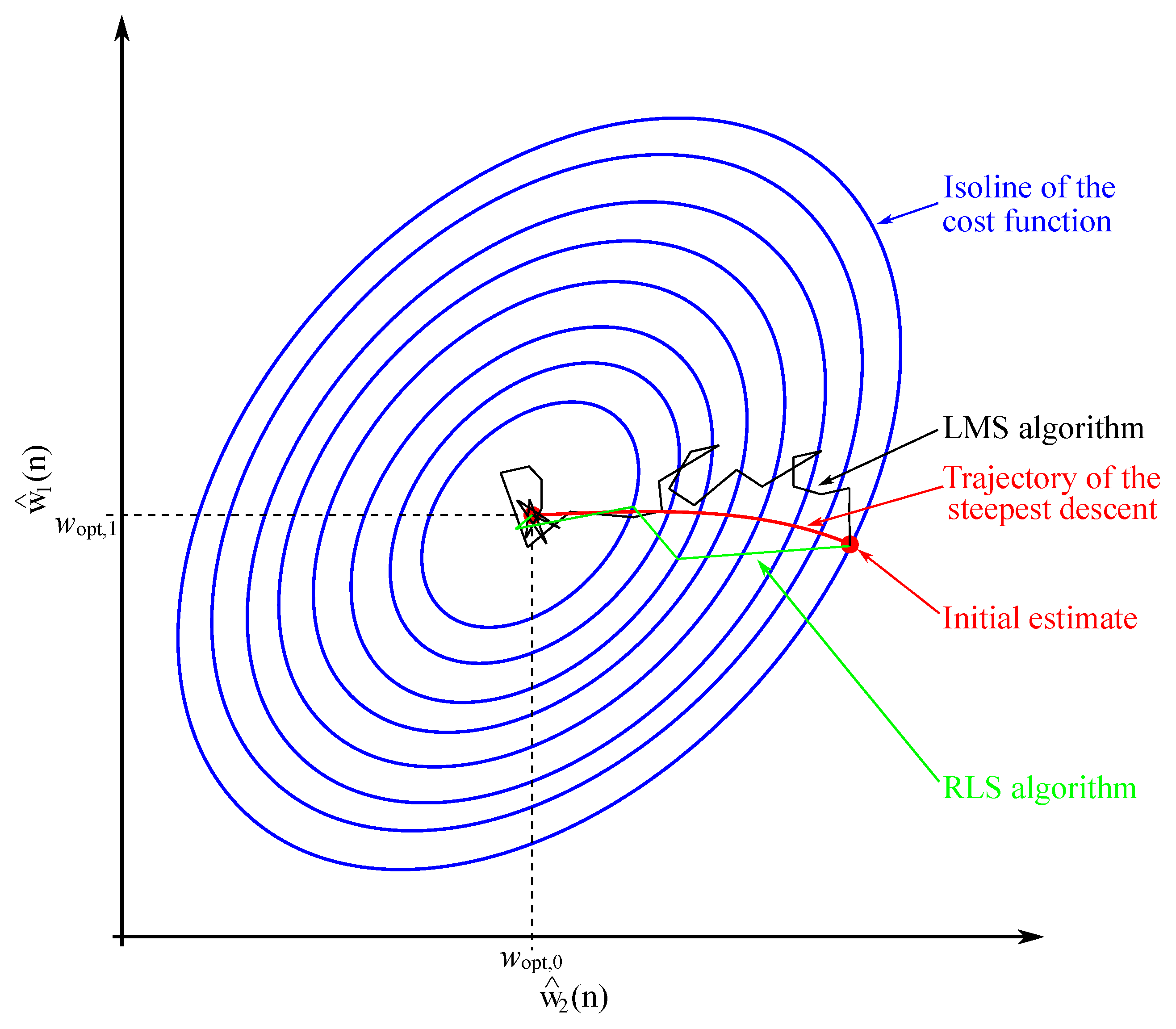
In Figure 7, the red line shows the optimal trajectory corresponding to the steepest process. Black (LMS algorithm) and green lines (RLS algorithm) represents a way for the coefficients estimation to get closer to the right (optimal) value. It takes several number of iterations n to get to optimal value. Also, it is evident that the given optimization process has its beginning provided by the initial estimation and its ending given by the terminal (optimized) estimation, i.e., $P=[w_{(\mathrm{opt},0)},w_{(\mathrm{opt},1)}]$.

4.4. Recursive Least Squares Algorithm

The RLS algorithm is a primary performer in the class of recursive algorithms, which are based on the theory of Kalman filtration, time averaging, and the least squares method. In contrast to the LMS algorithm, the RLS algorithm has its own statistic conception. It works with average values of quantities, which are calculated from time outputs [48].

For RLS algorithm implementation, the following steps have to be taken in this order:

• The filter output is calculated using filter weights from the previous iteration and the present input vector:

  $${\overrightarrow{y}}_{\mathrm{n}-1}\left(n\right)={\overrightarrow{w}}^{\mathrm{T}}(n-1)\overrightarrow{x}\left(n\right).$$

  (47)
• The vector of the mean gain is estimated using the following equation:

  $$\genfrac{}{}{0pt}{}{\overrightarrow{u}\left(n\right)={\tilde{\psi }}_{\lambda }^{-1}(n-1)\overrightarrow{x}\left(n\right),}{\overrightarrow{k}\left(n\right)=\frac{1}{\lambda +{\overrightarrow{x}}^{\mathrm{T}}\left(n\right)\overrightarrow{u}\left(n\right)}\overrightarrow{u}\left(n\right).}$$

  (48)
• The value of the estimated error is calculated according to following equation:

  $${\overrightarrow{e}}_{\mathrm{n}-1}\left(n\right)=d\left(n\right)-{\overrightarrow{y}}_{\mathrm{n}-1}\left(n\right).$$

  (49)
• The filter weights vector is updated using Equation (49) and the vector of the gain is calculated from Equation (47):

  $$\overrightarrow{w}\left(n\right)={\overrightarrow{w}}^{\mathrm{T}}(n-1)+k\left(n\right){\overrightarrow{e}}_{\mathrm{n}-1}\left(n\right).$$

  (50)
• The inverse matrix is computed according to following equation:

  $${\tilde{\psi }}_{\lambda }^{-1}\left(n\right)={\lambda }^{-1}({\tilde{\psi }}_{\lambda }^{-1}(n-1)-\overrightarrow{k}\left(n\right)[x^{\mathrm{T}}\left(n\right){\tilde{\psi }}_{\lambda }^{-1}(n-1)]).$$

  (51)

4.5. Discussion of the Choice of Coefficient $\lambda$ Value

In [78], the coefficient $\lambda$ is labeled as the so-called forgetting coefficient, taking values $\lambda \in (0,1\rangle$. If $\lambda =1$, then we talk about the estimation without forgetting. Due to the form ${\lambda }^{\mathrm{n}-\mathrm{i}}$, we can speak of weighting. The input values of the individual signal before $i=1$ are considered as zero; the values from the last n sets of values are significant. So, the previous autocorrelation matrix or correlation vector tends to be weighted, adding a correction for the actual values of the autocorrelation matrix or the correlation vector.

During practical implementation, we usually take into account values from $\lambda =0.98$ to $\lambda =1$. For small values of the coefficient $\lambda$, a small contribution of the previous samples into the covariance matrix exists. The filter is more sensitive to the actual samples. When $i-n$, i.e., ${\lambda }^{\mathrm{n}-\mathrm{n}}={\lambda }^0=1$, the mathematical description of the RLS algorithm is reduced to the description of LMS algorithm $[\Delta \left(n\right)={\lambda }^{\mathrm{n}-(\mathrm{i}=\mathrm{n})}=1]$.

4.6. Comparison of Mathematical Requirements

From the point of view of the implementation of the adaptive algorithms into digital signal processing (DSP), the computational cost and the memory requirements are especially important. These parameters are shown in

Table 1. Computational cost of the least mean squares (LMS) and recursive least mean squares (RLS) algorithms.

Algorithm	Plus/Minus in One Iteration	Multiplication in One Iteration	Memory Requirements
LMS	M + 1	2M	2M
RLS	M2 + M	2M2 + 3M + 50	M2 + 3M

, where M is the filter order.

By comparing the mathematical requirements, we can conclude that the RLS algorithm, which obtains better results than the LMS algorithm, has a high computational cost, which has an impact on the hardware requirements (processor and memory) the algorithm works on.

5. Experiments

Figure 8 shows the block diagram of the experiments, which were made with measured data (PFC is power factor correctio). During the experiments, both voltage and current on one-phase load were measured using National Instruments data acquisition hardware. The voltage was measured by an NI 9225 voltage input module and the current was measured by an NI 9227 current input module. Both NI 9225 and NI 9227 modules were plugged into a cDAQ 9185 chassis, and the chassis was connected to a PC by Ethernet. Voltage and current modules were configured to measure instant voltage and current values using simultaneous sampling with a sampling rate of 50 kSamples/s per channel. The software uses a time window Tw of 10 periods of the fundamental frequency (200 ms for a 50 Hz frequency) according to the IEC 61000-4-30 Ed.2.0. The amplitude of the fundamental harmonic, which serves as the amplitude of the reference sinus waveform, is settled using FFT.

The compensating current is obtained based on the sinusoidal reference current, the nonlinear current of the load, and the settings of the adaptive filter. The compensating current, which is obtained by the adaptive filter, is sent to the inverter, where the compensating current is generated, and then it is sent in the opposite phase to the PCC. However, we did not use the inverter, and were working in simulation mode when the delay of 100 $\mathsf{\mu }$s was implemented. A 100 $\mathsf{\mu }$s delay value was chosen because this value will also be performed in our modular inverter. After injecting compensation current, the sinusoidal waveform of the current in the electrical network should occur. Then, the parameters evaluating the filtration quality are computed. Loading of loads from the recorded data was made as if the loads were plugged into a socket. We did not work with the voltage because we are not able to observe a reverse effect of the current after compensation, when a deformation adjustment would occur, without the inverter.

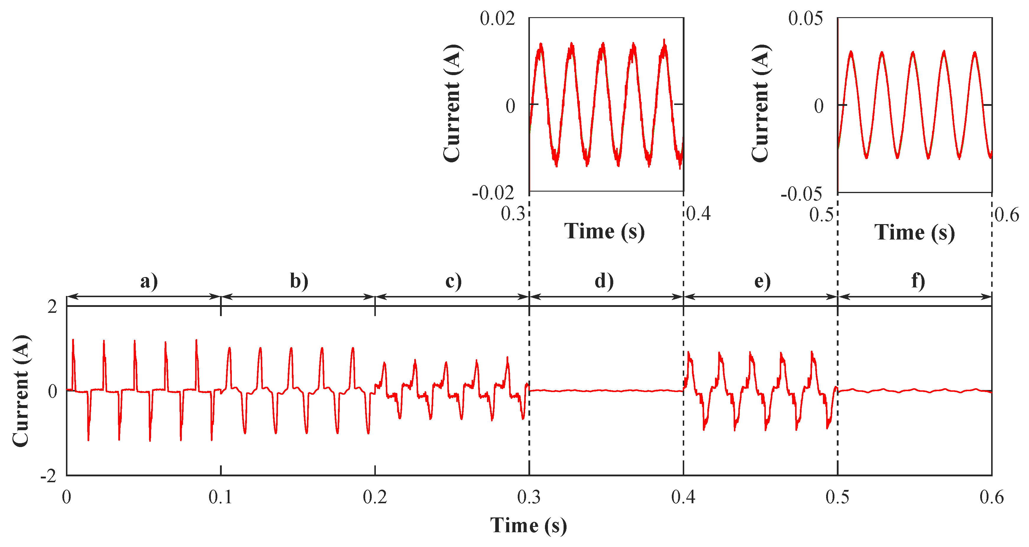
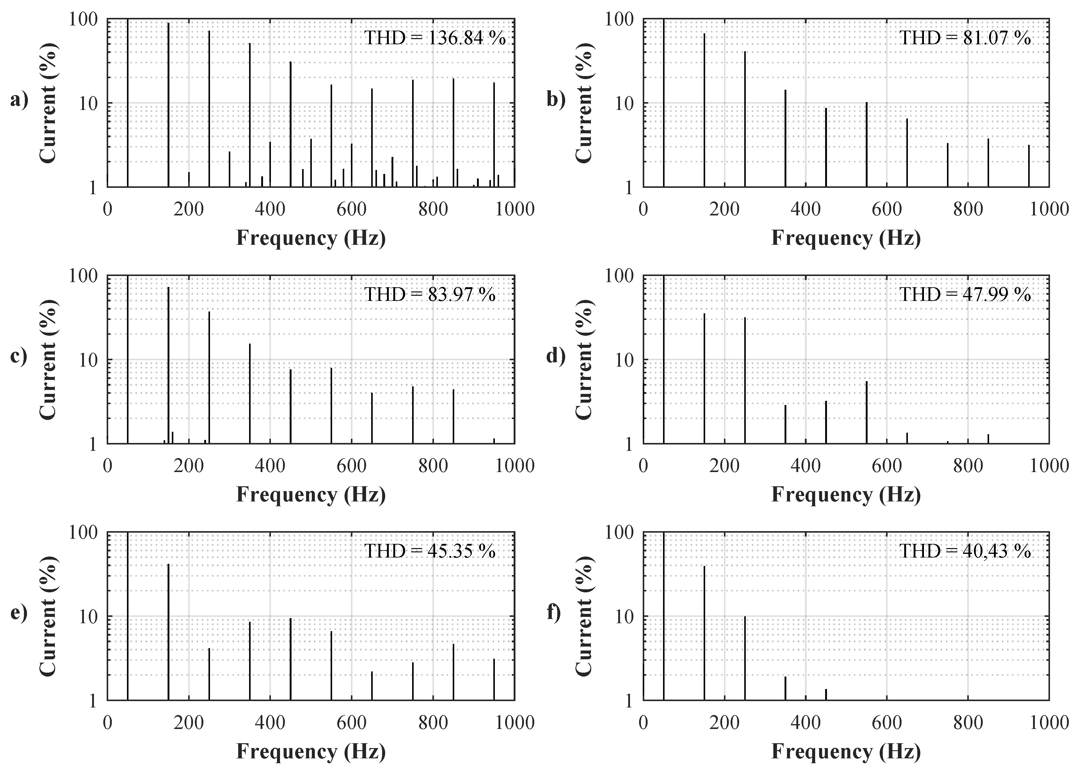
Figure 9 shows the one-phase waveform of the current with a substantial distortion of six nonlinear loads when each load has a time window length 100 ms. These loads were immediately changed for the verification of the robustness of the adaptive algorithm. The THD of the signal shown in Figure 9 is 63.27%. Figure 10 shows the FFT and THD for each load, in lengths of 100 ms.

Voltage input module NI 9225 has three direct voltage inputs. The incoming analog signal on each channel was conditioned, buffered, and then sampled by a 24-bit Delta-Sigma AD converter. The operating input range of NI 9225 is 850 Vpp (peak–peak). Loads were connected to a low-level distribution system with a nominal voltage of 230 V, 50 Hz, and this voltage was measured.

Current input module NI 9227 has four direct current inputs using a 12 m$\Omega$ shunt resistor as a current sensor. The incoming analog signal on each channel was conditioned, buffered, and then sampled by a 24-bit Delta-Sigma AD converter. The operating input range of NI 9227 is 28 App(peak–peak). Thanks to the enormous dynamic range of the 24-bit AD converter, the typical scaling coefficient (SC) was 1.785 $\mathsf{\mu }$A/LSB.

$$SC=\frac{I_{\mathrm{pp}}}{2^{\mathrm{N}}}=\frac{28}{2^{24}}=1.785\mathsf{\mu }\mathrm{A}.$$

(52)

From the set of loads presented in Figure 9, the smallest currents were measured for the following two loads: (d) HI-FI amplifier in standby mode had a peak–peak current of 30 mA and (f) the audio-tape recorderhad the peak–peak current of 80 mA. From the information above can be calculated the number of AD converter levels used to represent the smallest measured current, 30 mA${}_{\mathrm{pp}}$:

$$\frac{30\mathrm{m}{\mathrm{A}}_{\mathrm{pp}}}{1.785\mathsf{\mu }\mathrm{A}}=16806\mathrm{levels}.$$

(53)

To calculate the AD converter output word width from the known number of AD converter levels, the following formula can be used:

$$I={\log }_{2}16806=14.037\mathrm{bit}.$$

(54)

From this formula, it is evident that even the measured current peak-to-peak value (30 m${\mathrm{A}}_{\mathrm{pp}}$) is very small in comparison with the input range of the current module (28 A). Thanks to the huge dynamic range of the 24-bit AD converter used, the small signal is theoretically divided into 16806 levels and this corresponds to 14-bit AD converter.

For the measurement equipment, the effective number of bits (ENOB) has to be considered to respect the whole signal-chain and the real AD converter parameters. In the documentation for NI 9227, the ENOB cannot be found, but even subtracting 4 bits because of noise, the smallest measured signal was converted into digital form using a 14 − 4 = 10 bit AD converter. Regular oscilloscopes use 8 bit AD converters, the high-end oscilloscopes use 10 bit AD converters, and only the best oscilloscopes use 12 bit AD converters [79].

6. Results

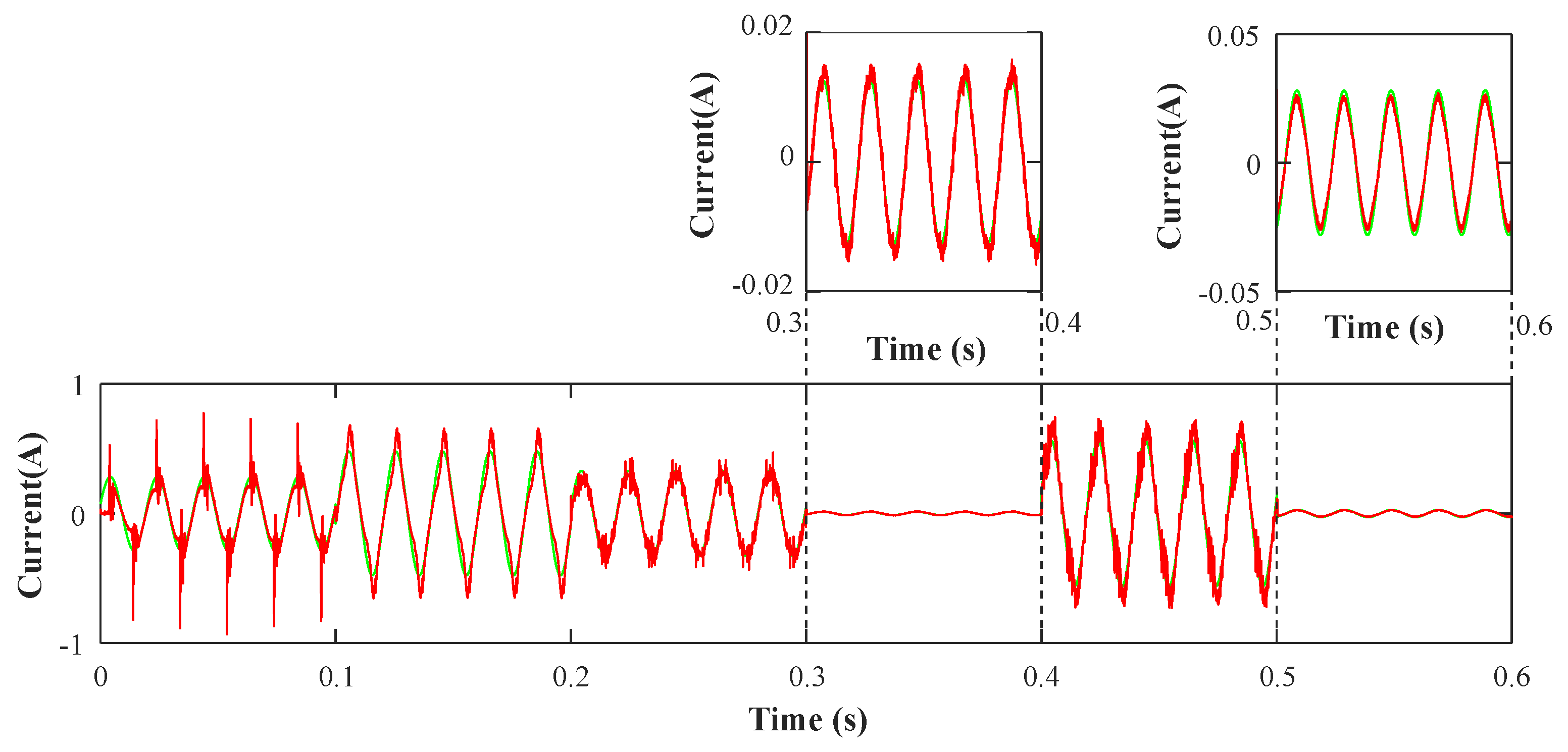
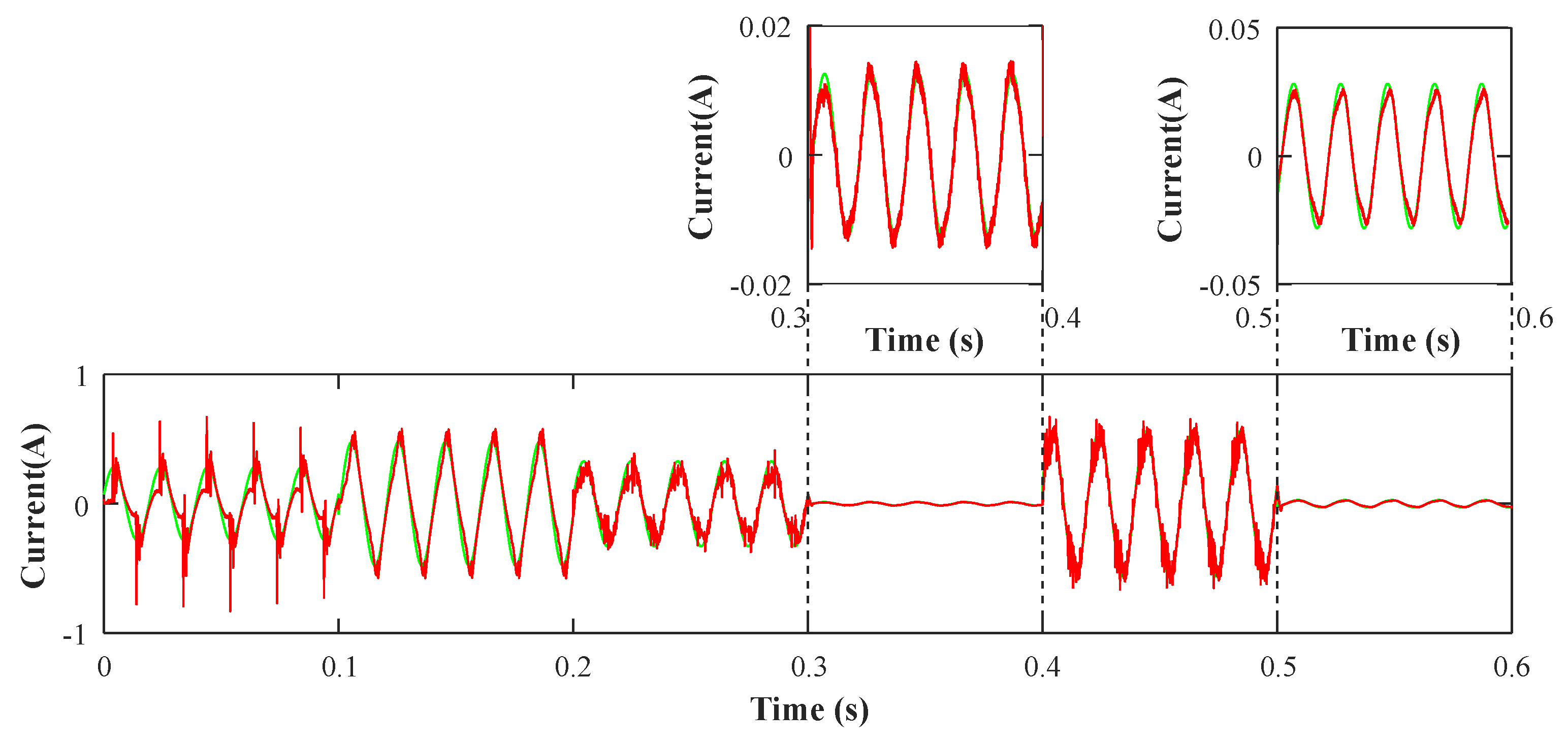
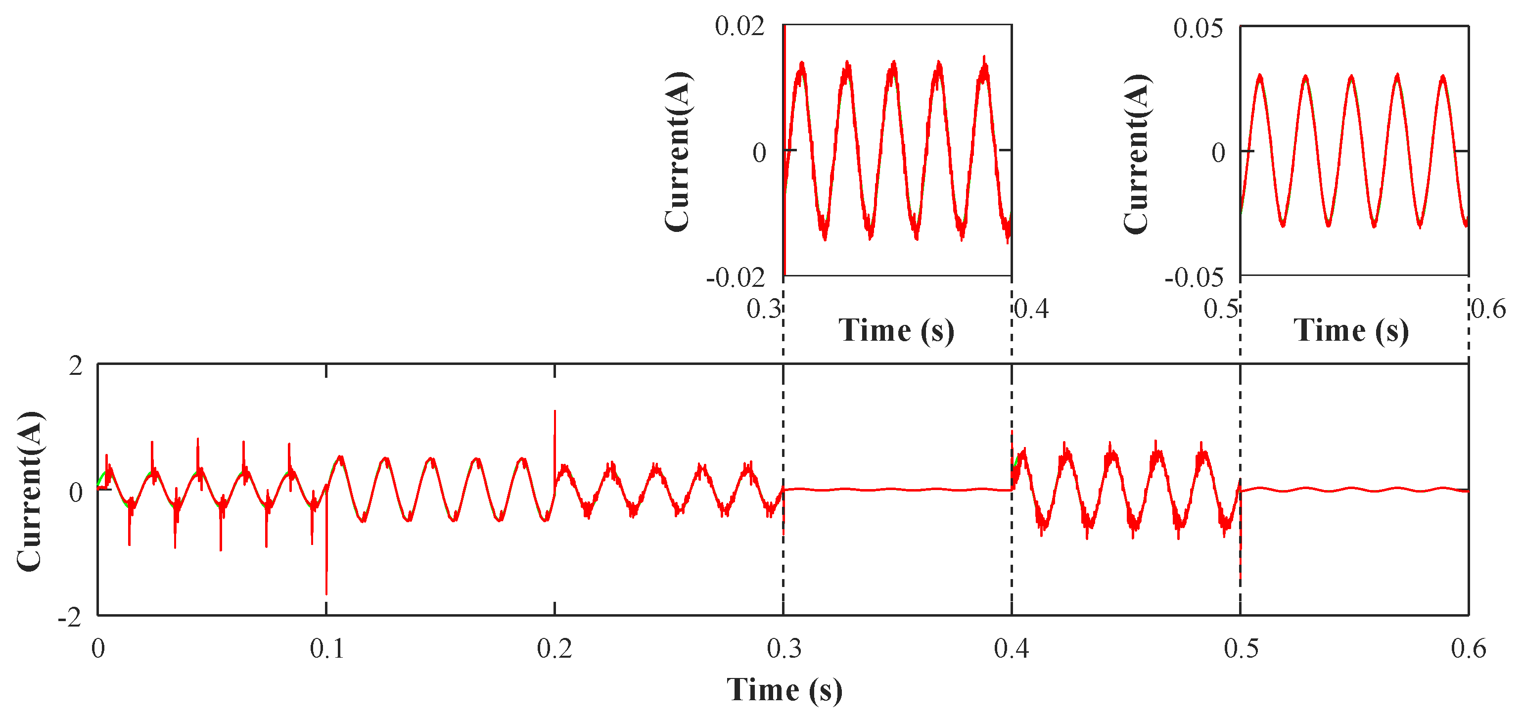
For the purpose of simulation, a delay of 100 $\mathsf{\mu }$s was added, which corresponds to the delay of the inverter, on which we will apply the algorithms. This delay resulted in the current after compensation not having the clearly sinusoidal waveform that was obtained in the case of adaptive algorithms without delay. However, from the view of the THD, this is a substantial improvement, namely from 63.27 % to 12.51 % when using LMS; to 14.3 % when applying NLMS, and to 6.43 % when utilizing the RLS algorithm. Figure 11, Figure 12 and Figure 13 show the waveform of the reference (green) and input (red) signals after filtration. The overshoots in the first 100 ms are caused by the delay of the inverter and by the type of compensated load. The overshoots are not so evident in the case of other types of load.

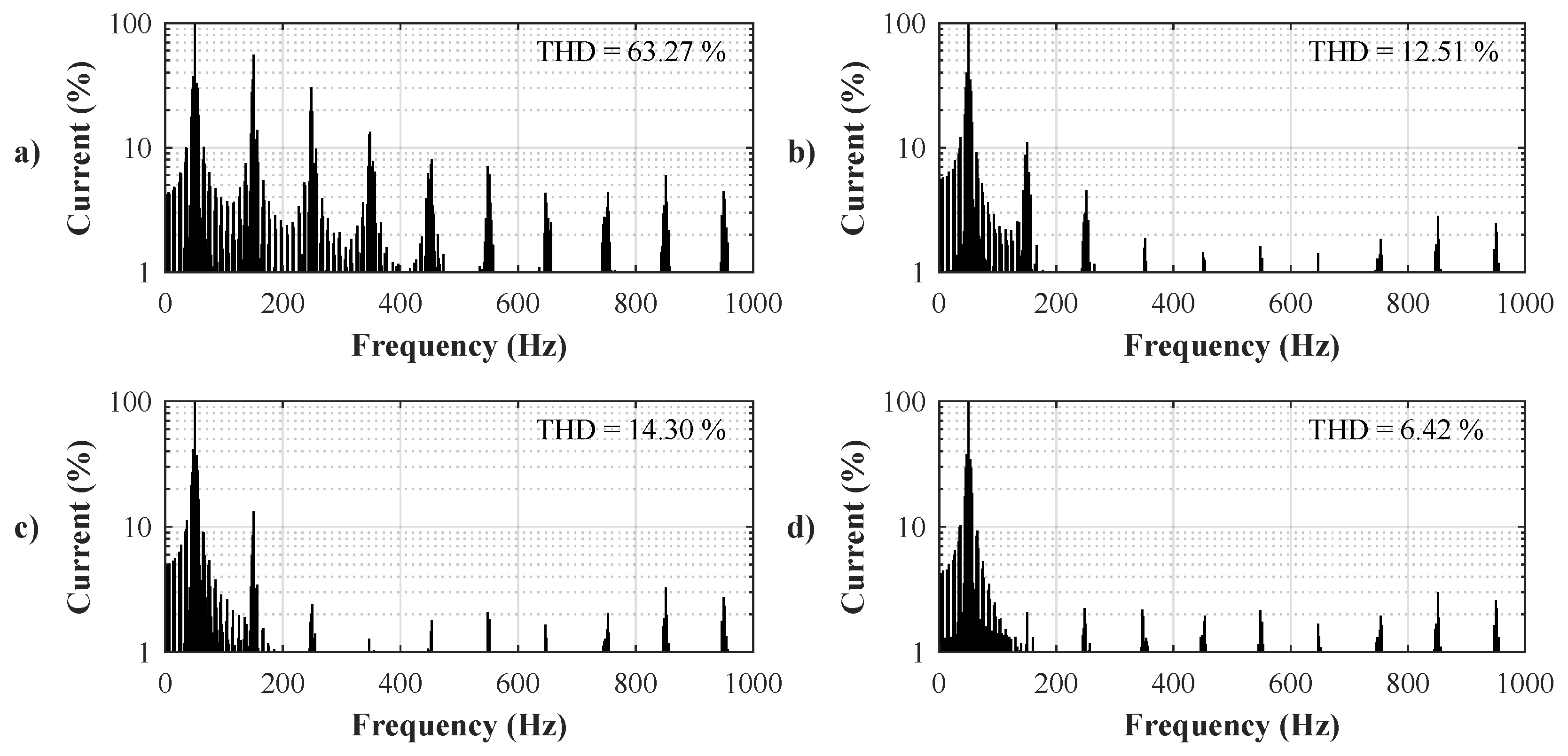
In Figure 14, the frequency spectras of the signal before and after filtration are shown. Before filtration, there exists a significant level of the third and fifth harmonics in the spectra. Those harmonics are suppressed by filtration using all three adaptive algorithms.

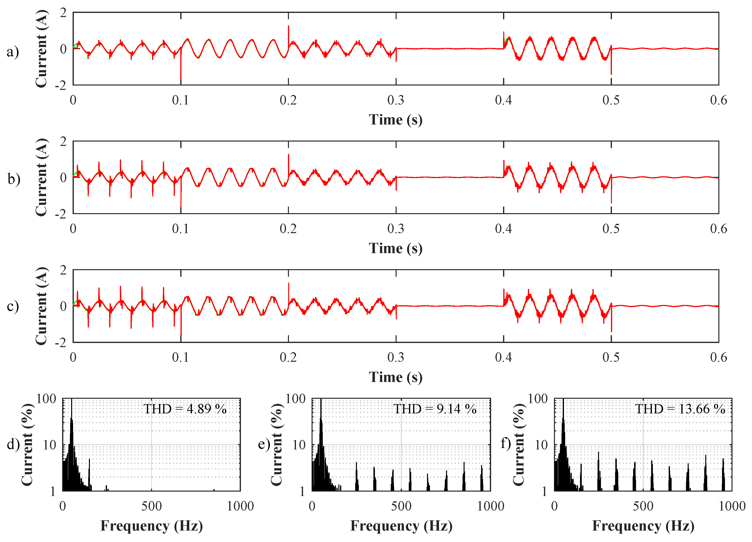
In Figure 15, you can see that the effect of the inverter delay on the THD was tested as part of adaptive filtration testing when the RLS algorithm was used. It was found that with a filter length of 2 and forgetting factor of 0.999, the delay set from 50 $\mathsf{\mu }$s to 200 $\mathsf{\mu }$s had an effect on the THD in the range of ±8%. This range varies depending on the filter settings, so the correct adaptive algorithm settings will be crucial for our application.

6.1. Total Harmonic Distortion

The THD defines the distortion of the sinus signal, indicated as a percentage. It is defined as a ratio of the sum of all powers of harmonic components and the power of the fundamental harmonic [80,81].

$$\mathrm{THD}=\frac{\sqrt{P_2^2+P_3^2+P_4^2+\cdots +P_{\mathrm{n}}^2}}{P_1}·100,$$

(55)

where $P_1$ is the power of the fundamental harmonic, and $P_2,\dots ,P_{\mathrm{n}}$ are the powers of higher harmonics.

6.2. Signal-to-Noise Ratio

The SNR is defined as the useful signal standoff from the noise, and it is indicated in decibels (dB). If the SNR is higher than 0 dB, the useful signal is greater than the noise. For the calculation, there is a need to know the ideal (reference) signal [82].

$${\mathrm{SNR}}_{\mathrm{OUT}}=10·{\log }_{10}\left(\frac{{\sum }_{\mathrm{i}=1}^{\mathrm{N}-1}{\left[{\mathrm{sig}}_{\mathrm{ideal}}\left(i\right)\right]}^2}{{\sum }_{\mathrm{i}=1}^{\mathrm{N}-1}{[{\mathrm{sig}}_{\mathrm{out}}\left(i\right)-{\mathrm{sig}}_{\mathrm{ideal}}\left(i\right)]}^2}\right).$$

(56)

6.3. Root Mean Square Error

The RMSE is defined as the mean quadratic error. It settles the difference between real and ideal values. The unit is established according the measured quantity [83].

$${\mathrm{RMSE}}_{\mathrm{OUT}}=\frac{1}{n}\sqrt{{\displaystyle \sum _{\mathrm{i}=1}^{\mathrm{n}}}{\left({\mathrm{sig}}_{\mathrm{out}}\left(i\right)-{\mathrm{sig}}_{\mathrm{ideal}}\left(i\right)\right)}^2}.$$

(57)

6.4. Percentage Root Mean Square Difference

The PRD is defined as the percent difference of the mean quadratic error [84,85].

$${\mathrm{PRD}}_{\mathrm{OUT}}=\sqrt{\frac{{\sum }_{\mathrm{i}=1}^{\mathrm{N}}{[{\mathrm{sig}}_{\mathrm{ideal}}\left(i\right)-{\mathrm{sig}}_{\mathrm{out}}\left(i\right)]}^2}{{\sum }_{\mathrm{i}=1}^{\mathrm{N}}{\mathrm{sig}}_{\mathrm{ideal}}^2\left(i\right)}}·100.$$

(58)

The filtration quality can be evaluated using the parameters THD, RMSE, and PRD when the values should be as low as possible and the parameter SNR when the values should be as high as possible.

The LMS and NLMS algorithms have a time of convergence under 100 ms with suitable settings and the RLS algorithm takes approximately 10 ms to stabilize the initial overcoming oscillation. Thus, we examined this time and the steady time separately.

From

Table 2. Results of the experiment using adaptive algorithms for the initial stage (from 0 to 100 ms).

LMS	Filter Length (-) = 10				Filter Length (-) = 30
$\mu$	THD	SNR${}_{\mathrm{OUT}}$	RMSE${}_{\mathrm{OUT}}$	PRD${}_{\mathrm{OUT}}$	THD	SNR${}_{\mathrm{OUT}}$	RMSE${}_{\mathrm{OUT}}$	PRD${}_{\mathrm{OUT}}$
(-)	(%)	(dB)	(A)	(%)	(%)	(dB)	(A)	(%)
0.01	31.41	7.25	0.0012	43.42	70.68	2.09	0.0022	78.57
0.001	49.31	4.19	0.0018	62.02	31.92	6.55	0.0013	47.06
0.005	28.69	7.57	0.0012	41.83	41.48	5.41	0.0015	53.65
NLMS	Filter Length (-) = 50				Filter Length (-) = 100
$\mu$	THD	SNR${}_{\mathrm{OUT}}$	RMSE${}_{\mathrm{OUT}}$	PRD${}_{\mathrm{OUT}}$	THD	SNR${}_{\mathrm{OUT}}$	RMSE${}_{\mathrm{OUT}}$	PRD${}_{\mathrm{OUT}}$
(-)	(%)	(dB)	(A)	(%)	(%)	(dB)	(A)	(%)
0.01	56.43	4.38	0.0017	60.38	55.95	4.33	0.0017	60.78
0.001	52.16	4.07	0.0018	62.57	44.98	4.31	0.0017	60.85
0.005	42.34	5.61	0.0015	52.44	38.59	5.90	0.0014	50.70
RLS	Filter Length (-) = 2				Filter Length (-) = 30
$\lambda$	THD	SNR${}_{\mathrm{OUT}}$	RMSE${}_{\mathrm{OUT}}$	PRD${}_{\mathrm{OUT}}$	THD	SNR${}_{\mathrm{OUT}}$	RMSE${}_{\mathrm{OUT}}$	PRD${}_{\mathrm{OUT}}$
(-)	(%)	(dB)	(A)	(%)	(%)	(dB)	(A)	(%)
0.99	84.37	1.41	0.0024	84.97	Unstable	Unstable	Unstable	Unstable
0.999	29.63	8.41	0.0011	37.98	29.55	7.95	0.0011	40.06
0.9999	31.71	8.10	0.0011	39.36	31.29	7.71	0.0011	41.15
1	31.95	8.06	0.0011	39.52	31.52	7.68	0.0012	41.31

$\mu$ is the step size; $\lambda$ is the forgetting factor.

and

Table 3. Results of the experiment using adaptive algorithms for a settled filter (from 100 to 600 ms).

LMS	Filter Length (-) = 10				Filter Length (-) = 30
$\mu$	THD	SNR${}_{\mathrm{OUT}}$	RMSE${}_{\mathrm{OUT}}$	PRD${}_{\mathrm{OUT}}$	THD	SNR${}_{\mathrm{OUT}}$	RMSE${}_{\mathrm{OUT}}$	PRD${}_{\mathrm{OUT}}$
(-)	(%)	(dB)	(A)	(%)	(%)	(dB)	(A)	(%)
0.01	19.33	8.65	0.00060	36.95	37.03	5.21	0.00089	54.89
0.001	5.96	18.08	0.00020	12.47	7.59	14.17	0.00032	19.57
0.005	10.86	12.69	0.00037	23.19	26.68	6.92	0.00073	45.09
NLMS	Filter Length (-) = 50				Filter Length (-) = 100
$\mu$	THD	SNR${}_{\mathrm{OUT}}$	RMSE${}_{\mathrm{OUT}}$	PRD${}_{\mathrm{OUT}}$	THD	SNR${}_{\mathrm{OUT}}$	RMSE${}_{\mathrm{OUT}}$	PRD${}_{\mathrm{OUT}}$
(-)	(%)	(dB)	(A)	(%)	(%)	(dB)	(A)	(%)
0.01	24.92	9.37	0.00055	33.99	24.03	9.93	0.00051	31.89
0.001	8.79	11.70	0.00042	26.00	8.50	11.92	0.00041	25.35
0.005	13.44	11.23	0.00044	27.44	12.58	12.76	0.00037	23.02
RLS	Filter Length (-) = 2				Filter Length (-) = 30
$\lambda$	THD	SNR${}_{\mathrm{OUT}}$	RMSE${}_{\mathrm{OUT}}$	PRD${}_{\mathrm{OUT}}$	THD	SNR${}_{\mathrm{OUT}}$	RMSE${}_{\mathrm{OUT}}$	PRD${}_{\mathrm{OUT}}$
(-)	(%)	(dB)	(A)	(%)	(%)	(dB)	(A)	(%)
0.99	40.65	3.57	0.00107	66.32	Unstable	Unstable	Unstable	Unstable
0.999	5.40	16.92	0.00023	14.26	7.55	16.44	0.00024	15.07
0.9999	7.11	18.23	0.00020	12.27	6.89	18.25	0.00020	12.24
1	7.50	18.08	0.00020	12.47	7.38	18.13	0.00020	12.41

$\mu$ is the step size; $\lambda$ is the forgetting factor.

, it can be seen that during the application of the LMS and NLMS algorithms, the THD is lower with a smaller step size. However, there is a longer time of convergence. For this reason, it is suitable to also compare the signal based on other parameters, such as SNR, RMSE, or PRD. Therefore, the most suitable settings of the LMS algorithm are a filter length of 10 and a step size of 0.001, and for the NLMS algorithm, a filter length of 100 and a step size of 0.001.

Table 2 and Table 3 lead to the conclusion that in the case of the RLS algorithm, it is not appropriate to set the value of the forgetting factor under 0.999 because these settings are non-stable or the parameters of the electrical network get worse. The best results were obtained using a forgetting factor of 0.999. The size of the filter length has an impact primarily in transitions where the amplitude changes, and in the case of a large filter length, the overcoming oscillations, which can reach up to multiple of the desired amplitude, occur.

6.5. Discussion

The designed conception, “least mean squares and recursive least squares algorithms for total harmonic distortion reduction using shunt active power filters control”, can also be used in a three-phase system. It is obvious that the proposal of three independent adaptive systems is needed for the three-phase design. The authors have solved the problematics in [40,41,42,46,48].

The next objective of the research, which will continue on from this study, will be the construction of a proper adaptive modular inverter. Different methods of SAPF control will be tested based on this system. The authors will focus on the development of a current generator designed to inject harmonics into the power grid and a set of nonlinear loads. The system will contain three independent one-phase generators and a module with a separate chokefor the possibility of inserting a defined impedance in the power grid. The generators can be used individually in a one-phase power grid or as a common assembly in a three-phase power grid. It will then be possible to test on this system.

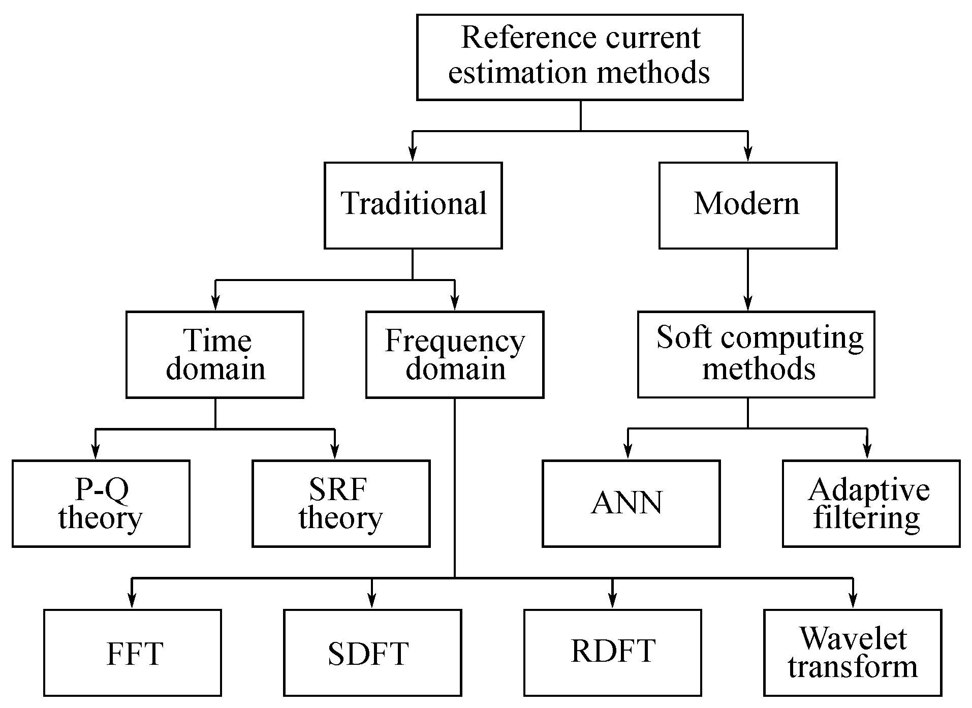
In the authors’ opinion, a comparative study of all methods mentioned above (traditional and modern) should be the object of subsequent research (see Figure 16), where ANN is artificial neural network, SRF is synchronous reference frame, SDFT is sliding discrete Fourier transform, and RDFT is recursive discrete Fourier transform. Currently, only a limited amount of comparative studies have been conducted, e.g., [86,87]. It is evident that the advanced techniques of signal processing are beginning to be applied in the SAPF control area, where they are still new. Nowadays, no comparative studies, which would compare the individual methods from the view of dynamic properties, THD improvement, implementation complexity, etc., exist.

Current trends in the domain of advanced methods of signal processing show that it would be possible to use some of the soft-computing methods for SAPF control [86,88], namely

• Adaptive systems [89,90,91,92,93],
• Methods based on techniques of artificial intelligence [94,95,96,97,98].

7. Conclusions

Within the experiments conducted, the simulation of an adaptive system, which was used to test the representatives of both basic families of adaptive algorithms, LMS and RLS, was undertaken. This system was used for the suppression of higher harmonic components. The practical use may rest in the suppression of higher harmonics and reactive power in an electrical network, primarily in an industry where nonlinear loads are abundantly represented.

The system was tested using real data, which were measured on consumer electronics. In the case of the LMS algorithm, the impact of the filter length and size of the convergence constant on the properties of the examined system was evaluated, specifically the signal distortion and the convergence time. It was shown that the requirements for these two properties are contradictory. By setting the filter length and the convergence constant, we can get either a system with fast adaptation but with a high distortion value, or the converse. In the case of the RLS algorithm, the impact of the filter length and the forgetting factor, which determines how many samples the system remembers, were examined. With an increasing filter length, higher overcoming oscillations occurred with changes in amplitude. With a decreasing value of the forgetting factor, the algorithm was more sensitive to recent samples, and it did not reach the desired accuracy, or it did not become stable.

Thus, in general, the RLS algorithm was found to be faster, and it showed better filtration results but at the expense of computational difficulty. The LMS algorithm did not have as good results as the RLS algorithm, but due to its low computational cost, it is suitable for practical use. In the future, we can expect an increase in computing power, which will lead to a more powerful DSP. Thus, the requirement of low computational costs for individual algorithms will disappear, and it will be possible to realize more powerful algorithms.

References

- Montero, M.I.M.; Cadaval, E.R.; Gonzalez, F.B. Comparison of control strategies for shunt active power filters in three-phase four-wire systems. IEEE Trans. Power Electron. 2007, 22, 229. [Google Scholar] [CrossRef]
- Kanjiya, P.; Khadkikar, V.; Zeineldin, H.H. Optimal control of shunt active power filter to meet IEEE Std. 519 current harmonic constraints under nonideal supply condition. IEEE Trans. Ind. Electron. 2015, 62, 724–734. [Google Scholar] [CrossRef]
- Mehrasa, M.; Pouresmaeil, E.; Zabihi, S.; Rodrigues, E.M.; Catalao, J.P. A control strategy for the stable operation of shunt active power filters in power grids. Energy 2016, 96, 325–334. [Google Scholar] [CrossRef]
- Panigrahi, R.; Subudhi, B.; Panda, P.C. A robust LQG servo control strategy of shunt-active power filter for power quality enhancement. IEEE Trans. Power Electron. 2016, 31, 2860–2869. [Google Scholar] [CrossRef]
- Rahman, N.F.A.; Hamzah, M.K.; Noor, S.Z.M.; Hasim, A.S.A. Single-phase hybrid active power filter using single switch parallel active filter and simple passive filter. In Proceedings of the 2009 International Conference on Power Electronics and Drive Systems (PEDS), Taipei, Taiwan, 2–5 November 2009; pp. 40–45. [Google Scholar] [CrossRef]
- Korenc, V.; Holoubek, J. Reactive Power Compensation in Practice; Electronics Libraries: Prague, Czech Republic, 1999. [Google Scholar]
- Chen, M.H. Development of shunt-type three-phase active power filter with novel adaptive control for wind generators. Sci. World J. 2015, 2015, 963456. [Google Scholar] [CrossRef] [PubMed]
- Chavan, U.M.; Thorat, A.R.; Bhosale, S.S. Shunt Active Filter for Harmonic Compensation Using Fuzzy Logic Technique. In Proceedings of the 2018 International Conference on Current Trends towards Converging Technologies (ICCTCT), Coimbatore, Tamilnadu, India, 1–3 March 2018; pp. 1–6. [Google Scholar] [CrossRef]
- Bula, D.; Pasko, M. Model of hybrid active power filter in the frequency domain. Anal. Simul. Electr. Comput. Syst. 2015, 15–26. [Google Scholar] [CrossRef]
- Sawant, D.P.; Chavan, P.P. SRF Method for Compensation of Source Current Harmonics using Shunt Active Filter. Int. J. Innov. Technol. 2016, 4, 3652–3655. [Google Scholar]
- Afonso, J.L.; Couto, C.; Martins, J.S. Active filters with control based on the pq theory. IEEE Ind. Electron. Soc. Newslett. 2000, 47, 5–10. [Google Scholar]
- Revuelta, P.S.; Herrera, R.S. Application of the instantaneous power theories in load compensation with active power filters. In Proceedings of the 10th European Conference on Power Electronics and Applications, Toulouse, France, 2–4 Semptember 2003. [Google Scholar]
- Kim, H.; Akagi, H. The instantaneous power theory on the rotating pqr reference frames. In Proceedings of the IEEE 1999 International Conference on Power Electronics and Drive Systems, PEDS’99, Hong-Kong, China, 27–29 July 1999; Volume 1, pp. 422–427. [Google Scholar] [CrossRef]
- Diab, M.; El-Habrouk, M.; Abdelhamid, T.H.; Deghedie, S. Survey of Active Power Filters Configurations. In Proceedings of the 2018 IEEE International Conference on System, Computation, Automation and Networking (ICSCA), Pondicherry, India, 6–7 July 2018; pp. 1–14. [Google Scholar] [CrossRef]
- Thakor, N.V.; Zhu, Y.S. Applications of adaptive filtering to ECG analysis: noise cancellation and arrhythmia detection. IEEE Trans. Biomed. Eng. 1991, 38, 785–794. [Google Scholar] [CrossRef]
- Stein, J.Y. Digital Signal Processing: A Computer Science Perspective; John Wiley & Sons, Inc.: Hoboken, NJ, USA, 2000. [Google Scholar]
- Uncini, A. Fundamentals of Adaptive Signal Processing; Springer International Publishing: Cham, Switzerland, 2015. [Google Scholar]
- Taebi, A.; Mansy, H.A. Noise cancellation from vibrocardiographic signals based on the ensemble empirical mode decomposition. J. Biotechnol. Bioeng. 2017, 2, 00024. [Google Scholar] [CrossRef]
- Aslam, M.S.; Raja, M.A.Z. A new adaptive strategy to improve online secondary path modeling in active noise control systems using fractional signal processing approach. Signal Process. 2015, 107, 433–443. [Google Scholar] [CrossRef]
- Clarkson, P.M. Optimal and Adaptive Signal Processing; Routledge: Abingdon-on-Thames, UK, 2017. [Google Scholar]
- Mowlaee, P.; Saeidi, R.; Stylianou, Y. Advances in phase-aware signal processing in speech communication. Speech Commun. 2016, 81, 1–29. [Google Scholar] [CrossRef]
- Mars, P. Learning Algorithms: Theory and Applications in Signal Processing, Control and Communications; CRC Press: Hoboken, NJ, USA, 2018. [Google Scholar]
- Chan, W.; Jaitly, N.; Le, Q.; Vinyals, O. Listen, attend and spell: A neural network for large vocabulary conversational speech recognition. In Proceedings of the 2016 IEEE International Conference on Acoustics, Speech and Signal Processing (ICASSP), Shanghai, China, 20–25 March 2016; pp. 4960–4964. [Google Scholar] [CrossRef]
- Saegrov, A.; Kamben, R.U.S. Method and System for Long-Range Adaptive Mobile Beam-Forming Ad-Hoc Communication System With Integrated Positioning. U.S. Patent No. 9,516,513, 6 December 2016. [Google Scholar]
- Wang, J.; Su, W.; Sabatti, C.; Owen, A.B. Detecting Replicating Signals using Adaptive Filtering Procedures with the Application in High-throughput Experiments. arXiv 2016, arXiv:1610.03330. [Google Scholar]
- Imani, M.; Braga-Neto, U.M. Maximum-likelihood adaptive filter for partially observed boolean dynamical systems. IEEE Trans. Signal Process. 2017, 65, 359–371. [Google Scholar] [CrossRef]
- Shi, Y.; Shen, C.; Fang, H.; Li, H. Advanced control in marine mechatronic systems: A survey. IEEE/ASME Trans. Mechatron. 2017, 22, 1121–1131. [Google Scholar] [CrossRef]
- Srinivas, M.; Hussain, I.; Singh, B. Combined LMS–LMF-based control algorithm of DSTATCOM for power quality enhancement in distribution system. IEEE Trans. Ind. Electron. 2016, 63, 4160–4168. [Google Scholar] [CrossRef]
- Schmidt, M.; Le Roux, N.; Bach, F. Minimizing finite sums with the stochastic average gradient. Math. Program. 2017, 162, 83–112. [Google Scholar] [CrossRef]
- Ruder, S. An overview of gradient descent optimization algorithms. arXiv 2016, arXiv:1609.04747. [Google Scholar]
- Mandt, S.; Hoffman, M.D.; Blei, D.M. Stochastic gradient descent as approximate bayesian inference. J. Mach. Learn. Res. 2017, 18, 4873–4907. [Google Scholar]
- Wu, Z.; Shi, J.; Zhang, X.; Ma, W.; Chen, B.; Senior Member, I.E. Kernel recursive maximum correntropy. Signal Process. 2015, 117, 11–16. [Google Scholar] [CrossRef]
- Shanechi, M.M.; Orsborn, A.L.; Carmena, J.M. Robust brain-machine interface design using optimal feedback control modeling and adaptive point process filtering. PLoS Comput. Biol. 2016, 12, e1004730. [Google Scholar] [CrossRef]
- Wang, J.; Yu, C.; Li, S.E.; Wang, L. A forward collision warning algorithm with adaptation to driver behaviors. IEEE Trans. Intell. Transp. Syst. 2016, 17, 1157–1167. [Google Scholar] [CrossRef]
- Elobaid, L.M.; Abdelsalam, A.K.; Zakzouk, E.E. Artificial neural network-based photovoltaic maximum power point tracking techniques: A survey. IET Renew. Power Gener. 2015, 9, 1043–1063. [Google Scholar] [CrossRef]
- Ali, J.B.; Fnaiech, N.; Saidi, L.; Chebel-Morello, B.; Fnaiech, F. Application of empirical mode decomposition and artificial neural network for automatic bearing fault diagnosis based on vibration signals. Appl. Acoust. 2015, 89, 16–27. [Google Scholar] [CrossRef]
- Qiu, J.; Ding, S.X.; Gao, H.; Yin, S. Fuzzy-Model-Based Reliable Static Output Feedback H∞ Control of Nonlinear Hyperbolic PDE Systems. IEEE Trans. Fuzzy Syst. 2016, 24, 388–400. [Google Scholar] [CrossRef]
- Jain, L.C.; Kandel, A.; Teodorescu, H.N.L. Fuzzy and Neuro-Fuzzy Systems in Medicine; CRC Press: Boca Raton, FL, USA, 2017. [Google Scholar]
- Pothal, J.K.; Parhi, D.R. Navigation of multiple mobile robots in a highly clutter terrains using adaptive neuro-fuzzy inference system. Robot. Auton. Syst. 2015, 72, 48–58. [Google Scholar] [CrossRef]
- Martinek, R.; Manas, J.; Zidek, J.; Bilik, P. Power quality improvement by shunt active performance filters emulated by artificial intelligence techniques. In Proceedings of the 2nd International Conference on Advances in Computer Science and Engineering (CSE 2013), Los Angeles, CA, USA, 1–2 July 2013; Atlantis Press: Paris, France, 2013. [Google Scholar] [CrossRef]
- Martinek, R.; Vanus, J.; Kelnar, M.; Bilik, P. Control methods of active power filters using soft computing techniques. In Proceedings of the 8th International scientific symposium on electrical power engineering (Elektroenergetika), Stara Lesna, Slovakia, 16–18 September 2015; pp. 363–366. [Google Scholar]
- Martinek, R.; Vanus, J.; Bilik, P.; Stratil, T.; Zidek, J. An efficient control method of shunt active power filter using adaline. IFAC-PapersOnLine 2016, 49, 352–357. [Google Scholar] [CrossRef]
- Bhattacharya, A.; Chakraborty, C. A shunt active power filter with enhanced performance using ANN-based predictive and adaptive controllers. IEEE Trans. Ind. Electron. 2011, 58, 421–428. [Google Scholar] [CrossRef]
- Elmitwally, A.; Abdelkader, S.; El-Kateb, M. Neural network controlled three-phase four-wire shunt active power filter. IEE Proc. Gener. Transm. Distrib. 2000, 147, 87–92. [Google Scholar] [CrossRef]
- Hamadi, A.; Al-Haddad, K.; Rahmani, S.; Kanaan, H. Comparison of fuzzy logic and proportional integral controller of voltage source active filter compensating current harmonics and power factor. In Proceedings of the 2004 IEEE International Conference on Industrial Technology, 2004, IEEE ICIT’04, Hammamet, Tunisia, 8–10 December 2004; Volume 2, pp. 645–650. [Google Scholar] [CrossRef]
- Martinek, R.; Bilik, J. New Strategies for Application of Recursive Least Square Algorithm in Active Power Filters. In Proceedings of the 8th International Scientific Symposium on Electrical Power Engineering (Elektroenergetika), Stara Lesna, Slovakia, 16–18 September 2015; pp. 344–347. [Google Scholar]
- Tamboli, D.A.; Chile, R.H. Reference signal generation for shunt active power filter using adaptive filtering approach. In Proceedings of the 2015 International Conference on Industrial Instrumentation and Control (ICIC), Pune, India, 28–30 May 2015; pp. 766–770. [Google Scholar] [CrossRef]
- Martinek, R.; Zidek, J.; Bilik, P.; Manas, J.; Koziorek, J.; Teng, Z.; Wen, H. The use of lms and rls adaptive algorithms for an adaptive control method of active power filter. Energy Power Eng. 2013, 5, 1126. [Google Scholar] [CrossRef]
- Paclt, Z. Active Power Filter Control; CVUT in Prague: Praha, Czech Republic, 2011. [Google Scholar]
- Emadi, A.; Nasiri, A.; Bekiarov, S.B. Uninterruptible Power Supplies and Active Filters; CRC Press: Boca Raton, FL, USA, 2015. [Google Scholar]
- Koupeny, J. Control Algorithms of Active Filters; CVUT in Prague: Praha, Czech Republic, 2008. [Google Scholar]
- Zhao, H.J.; Pang, Y.F.; Qiu, Z.M.; Chen, M. Study on UPF harmonic current detection method based on DSP. J. Phys. Conf. Ser. 2006, 48, 1327. [Google Scholar] [CrossRef]
- CH, S.; Kusam, S.; Shekar, K.C. Shunt active filter algorithms for a three phase system fed to adjustable speed drive. Int. J. Eng. Sci. Technol. 2011, 3, 7577–7586. [Google Scholar]
- Akagi, H.; Kanazawa, Y.; Nabae, A. Instantaneous reactive power compensators comprising switching devices without energy storage components. IEEE Trans. Ind. Appl. 1984, 3, 625–630. [Google Scholar] [CrossRef]
- Akagi, H.; Watanabe, E.H.; Aredes, M. Instantaneous Power Theory and Applications to Power Conditioning; John Wiley & Sons: Hoboken, NJ, USA, 2017; Volume 62. [Google Scholar]
- Bhattacharya, S.; Divan, D.M.; Banerjee, B. Synchronous frame harmonic isolator using active series filter. In Proceedings of the European Conference on Power Electronics and Applications, Firenze, Italy, 1–30 September 1991; Volume 3, p. 30. [Google Scholar]
- Pinto, J.G.; Neves, P.; Pregitzer, R.G.; Monteiro, L.F.; Afonso, J.L. Single-phase shunt active filter with digital control. Renew. Energies Power Qual. J. 2007, 1, 619–624. [Google Scholar] [CrossRef]
- Haque, M.T. Single-phase pq theory for active filters. In Proceedings of the 2002 IEEE Region 10 Conference on Computers, Communications, Control and Power Engineering, TENCOM’02, Beijing, China, 28–31 October 2002; Volume 3, pp. 1941–1944. [Google Scholar] [CrossRef]
- Paulo, S.D. Adaptive Filtering: Algorithms and Practical Implementation; The International Series in Engineering and Computer Science; Springer: New York, NY, USA, 2008; pp. 23–50. [Google Scholar]
- Poularikas, A.D.; Ramadan, Z.M. Adaptive Filtering Primer with MATLAB; CRC Press: Boca Raton, FL, USA, 2017. [Google Scholar]
- Arenas-Garcia, J.; Azpicueta-Ruiz, L.A.; Silva, M.T.; Nascimento, V.H.; Sayed, A.H. Combinations of adaptive filters: performance and convergence properties. IEEE Signal Process. Mag. 2016, 33, 120–140. [Google Scholar] [CrossRef]
- Sayed, A.H. Adaptive Filters; John Wiley & Sons: Hoboken, NJ, USA, 2011. [Google Scholar]
- Farhang-Boroujeny, B. Adaptive Filters: Theory and Applications; John Wiley & Sons: Hoboken, NJ, USA, 2013. [Google Scholar]
- Bellanger, M.; Bellanger, M. Adaptive Digital Filters; CRS Press: Boca Raton, FL, USA, 2001. [Google Scholar] [CrossRef]
- Saxena, G.; Ganesan, S.; Das, M. Real time implementation of adaptive noise cancellation. In Proceedings of the 2008 IEEE International Conference on Electro/Information Technology, Ames, IA, USA, 18–20 May 2008; pp. 431–436. [Google Scholar] [CrossRef]
- Mitra, S.K.; Kuo, Y. Digital Signal Processing: A Computer-Based Approach; McGraw-Hill: New York, NY, USA, 2006; Volume 2. [Google Scholar]
- Ifeachor, E.C.; Jervis, B.W. Digital Signal Processing: A Practical Approach; Pearson Education: London, UK, 2002. [Google Scholar]
- Haykin, S.S.; Widrow, B. Least-Mean-Square Adaptive Filters; Wiley-Interscience: New York, NY, USA, 2003; Volume 31. [Google Scholar]
- Bershad, N.J.; Bermudez, J.C.M.; Tourneret, J.Y. An affine combination of two LMS adaptive filters—Transient mean-square analysis. IEEE Trans. Signal Process. 2008, 56, 1853–1864. [Google Scholar] [CrossRef]
- Sayed, A.H.; Kailath, T. A state-space approach to adaptive RLS filtering. IEEE Signal Process. Mag. 1994, 11, 18–60. [Google Scholar] [CrossRef]
- Dhiman, J.; Ahmad, S.; Gulia, K. Comparison between Adaptive filter Algorithms (LMS, NLMS and RLS). Int. J. Sci. Eng. Technol. Res. (IJSETR) 2013, 2, 1100–1103. [Google Scholar]
- Szopos, E.; Hedesiu, H. LabVIEW FPGA based noise cancelling using the LMS adaptive algorithm. Acta Tech. Napoc. Electron. Telecommun. 2009, 50, 5–8. [Google Scholar]
- Kehtarnavaz, N.; Gope, C. DSP system design using LabVIEW and Simulink: a comparative evaluation. In Proceedings of the 2006 IEEE International Conference on Acoustics Speech and Signal Processing Proceedings, Toulouse, France, 14–19 May 2006; Volume 2, p. II. [Google Scholar] [CrossRef]
- Tian, H.; Duan, L.J. Design of multifunctional digital filter based on LabVIEW. Electron. Meas. Technol. 2011, 3. Available online: http://en.cnki.com.cn/Article_en/CJFDTotal-DZCL201103016.htm (accessed on 14 April 2019).
- Duttweiler, D.L. Proportionate normalized least-mean-squares adaptation in echo cancelers. IEEE Trans. Speech Audio Process. 2000, 8, 508–518. [Google Scholar] [CrossRef]
- Song, I.; Park, P.; Newcomb, R.W. A normalized least mean squares algorithm with a step-size scaler against impulsive measurement noise. IEEE Trans. Circuits Syst. II Express Briefs 2013, 60, 442–445. [Google Scholar] [CrossRef]
- Douglas, S.C. A family of normalized LMS algorithms. IEEE Signal Process. Lett. 1994, 1, 49–51. [Google Scholar] [CrossRef]
- Krejca, L. Implementation of the Channel Equalization Algorithms Used in FMT Modulation. Master’s Thesis, VUT in Brno, Brno, Czech Republic, 2010. [Google Scholar]
- IEC 61000-4-30 Ed.2.0 Electromagnetic Compatibility (EMC): Part 4-30: Testing and Measurement Techniques—Power Quality Measurement Methods; International Electrotechnical Commission: Geneva, Switzerland, 2008; 134p, ISBN 2-8318-1002-0.
- Qian, S.; Madsen, K.N.; Lucia, W.A.N.U.S. Total Harmonic Distortion (THD) Controlled Clip Detector and Automatic Gain Limiter (AGL). U.S. Patent Application No. 10/079,578, 12 August 2018. [Google Scholar]
- Srndovic, M.; Familiant, Y.; Grandi, G.; Ruderman, A. Time-domain minimization of voltage and current total harmonic distortion for a single-phase multilevel inverter with a staircase modulation. Energies 2016, 9, 815. [Google Scholar] [CrossRef]
- Proakis, J.G. Digital Signal Processing: Principles Algorithms and Applications; Pearson Educ. India: Chennai, India, 2001. [Google Scholar]
- Willmott, C.J.; Matsuura, K. Advantages of the mean absolute error (MAE) over the root mean square error (RMSE) in assessing average model performance. Clim. Res. 2005, 30, 79–82. [Google Scholar] [CrossRef]
- Javaid, R.; Besar, R.; Abas, F.S. Performance evaluation of percent root mean square difference for ecg signals compression. Signal Process. Int. J. (SPIJ) 2008, 48, 1–9. [Google Scholar]
- Blanco-Velasco, M.; Cruz-Roldan, F.; Godino-Llorente, J.I.; Blanco-Velasco, J.; Armiens-Aparicio, C.; Lopez-Ferreras, F. On the use of PRD and CR parameters for ECG compression. Med. Eng. Phys. 2005, 27, 798–802. [Google Scholar] [CrossRef]
- Singh, H.; Kour, M.; Thanki, D.V.; Kumar, P. A Review on Shunt Active Power Filter Control Strategies. Int. J. Eng. Technol. 2018, 7, 121–125. [Google Scholar] [CrossRef]
- Bajaj, M.; Rautela, S.; Sharma, A. A comparative analysis of control techniques of SAPF under source side disturbance. In Proceedings of the 2016 International Conference on Circuit, Power and Computing Technologies (ICCPCT), Nagercoil, India, 18–19 March 2016; pp. 1–7. [Google Scholar] [CrossRef]
- Rajagopal, R.; Palanisamy, K.; Paramasivam, S. A Technical Review on Control Strategies for Active Power Filters. In Proceedings of the 2018 International Conference on Emerging Trends and Innovations In Engineering And Technological Research (ICETIETR), Ernakulam, India, 11–13 July 2018; pp. 1–6. [Google Scholar] [CrossRef]
- Mu, X.; Wang, J.; Wu, W.; Blaabjerg, F. A modified multifrequency passivity-based control for shunt active power filter with model-parameter-adaptive capability. IEEE Trans. Ind. Electron. 2018, 65, 760–769. [Google Scholar] [CrossRef]
- Salimi, M.; Soltani, J.; Zakipour, A. Experimental design of the adaptive backstepping control technique for single-phase shunt active power filters. IET Power Electron. 2017, 10, 911–918. [Google Scholar] [CrossRef]
- Prabha, D.; Jain, L. Modified Recursive Least Square Algorithm for THD Reduction using Shunt Active Power Filter in Grid. Int. J. Online Sci. 2019, 5, 8. [Google Scholar]
- Panigrahi, R.; Subudhi, B. Performance Enhancement of Shunt Active Power Filter Using a Kalman Filter-Based H∞ Control Strategy. IEEE Trans. Power Electron. 2017, 32, 2622–2630. [Google Scholar] [CrossRef]
- Terriche, Y.; Golestan, S.; Guerrero, J.M.; Vasquez, J.C. Multiple-Complex Coefficient-Filter-Based PLL for Improving the Performance of Shunt Active Power Filter under Adverse Grid Conditions. In Proceedings of the 2018 IEEE Power & Energy Society General Meeting (PESGM), Portland, OR, USA, 5–10 August 2018; pp. 1–5. [Google Scholar] [CrossRef]
- Ray, S.; Gupta, N.; Gupta, R.A. Modified Three-Layered Artificial Neural Network-Based Improved Control of Multilevel Inverters for Active Filtering. In Proceedings of the Soft Computing for Problem Solving, Tamil Nadu, India, 17–19 December 2018; Springer: Singapore, 2018; pp. 547–558. [Google Scholar] [CrossRef]
- Krismanto, A.U.; Lomi, A.; Hartungi, R. Artificial neural network-based harmonics extraction algorithm for shunt active power filter control. J. Karya Dosen ITN Malang 2017, 4, 273–289. [Google Scholar] [CrossRef]
- Fei, J.; Wang, T. Adaptive fuzzy-neural-network based on RBFNN control for active power filter. Int. J. Mach. Learn. Cybern. 2018, 112, 1–12. [Google Scholar] [CrossRef]
- Badoni, M.; Singh, B.; Singh, A. Implementation of echo-state network-based control for power quality improvement. IEEE Trans. Ind. Electron. 2017, 64, 5576–5584. [Google Scholar] [CrossRef]
- Musa, S.; Radzi, M.; Hizam, H.; Wahab, N.; Hoon, Y.; Zainuri, M. Modified synchronous reference frame based shunt active power filter with fuzzy logic control pulse width modulation inverter. Energies 2017, 10, 758. [Google Scholar] [CrossRef]
Figure 1.
Block diagram of a shunt active power filter (SAPF).
Figure 2.
Axis coordinates used in transformations.