Solar Irradiance Forecast Using Naïve Bayes Classifier Based on Publicly Available Weather Forecasting Variables

Abstract

This paper develops an approach for two-day-ahead global horizontal irradiance (GHI) forecast using the naïve Bayes classifier (NB). Based on publicly available weather forecasting information about temperature, relative humidity, dew point, and sky coverage, they are used as a training set in NB classification with hourly resolution. To reduce having two times with the same GHI affecting the classification in the proposed model, two characteristics of the GHI under different weather conditions are considered: The daylight variation and diurnal cycle. More importantly, NB’s independence assumption-based on simple Bayes’ theorem makes the process speed faster and less constrained than other classification algorithms. The forecast performance is verified with several error criteria from established analytical practices using relevant statistics. Moreover, commonly used forecasting error criteria are discussed. This NB model shows improved results regarding error criteria and a good agreement for a clear day that satisfies the guideline for the evaluation of two-days-ahead forecast, when compared with other recent techniques.

1. Introduction

This paper presents a study for solar irradiance forecasting in order to improve the operation of photovoltaic (PV) systems. Presently, global environmental issues and energy demand are promoting the use of clean and sustainable energy sources on local utility grids. Among alternative energy sources, PV power is desirable for its minimal environmental impact, reduced reliance on oil, and improved secure electricity supply [1]. The contribution of power production to PV systems in electricity grids may likely increase in the future partly motivated by lower costs and up to 22% cell-efficiency improvement [2], with further cost reductions and efficiency improvements expected in the future. However, as grid-connected PV systems increase, grid operators and system planners will also be more concerned about PV systems’ power output fluctuation. Since PV power output may vary significantly depending on the solar irradiance, some potential issues could be expected by utility-grid operators associated with scheduling primary and spinning reserve capacity and voltage control. As an alternative plan, energy storage can compensate solar irradiance variability [3,4], but, in terms of developing adequate dispatching plans and transmission scheduling, a-day-ahead market expectations still require accurate solar irradiance forecast techniques with an hourly resolution [5].

Until recently, many studies have worked on forecasting global horizontal irradiance (GHI), which represents the total solar irradiance from the entire sky on a horizontal surface. It includes the sum of the direct-beam, the diffuse radiation from atmospheric scattering, and reflections and the reflected solar radiation from the ground [6]. These solar forecast techniques can be divided into two classes by data resolution. For high resolution (i.e., less than one hour), most time series techniques, such as regression, autoregressive integrated moving average (ARIMA) [7], artificial neural networks (ANN), and hybrid models that are combination of regressions with ANN, show good accuracy compared to the reference model in [8]. For the a-day-ahead forecast with hourly resolution, the study in [9] forecasted solar irradiance using ANN with a multilayer perception (MLP) model during sunny and cloudy days. For the sunny days, the forecast accuracy is verified with a correlation coefficient of 98.95% to 99.96% and a relative mean bias error (RMBE) of—6.43% to 32% (this negative error means under-estimated result). Similar to [9], the study in [10] proposed solar power forecast using ANN in several weather types. For sunny days, the correlation coefficient ranged from 98.43% to 99.39% and the mean absolute percentage error (MAPE) was between 8.29% and 10.8%. However, larger errors were observed in partially cloudy days because of weather forecast uncertainty in the cloud cover percentage during this type of days. That is, errors in cloud cover percentage are more likely in partially cloudy days than errors when a clear day is forecasted. The studies in [11,12] also developed solar irradiance forecast hour-by-hour or day-by-day using ANN. However, they produced results with large errors given the previous poorly forecasted value.

The ANN-forecast techniques are frequently used in many areas and work well, but they also have drawbacks. Complicated architecture, a large training data set, and choosing the optimal number of hidden layers and input nodes for the better results are still issues that need to be addressed. Furthermore, the use of different test criteria (i.e., comparison to the unclear reference model, normalization factors, or test duration) or performance testing under the several defined weather types (i.e., sunny, foggy, rainy, cloudy) make it difficult to compare with other developed models and to understand certain real-time weather patterns.

In order to solve these problems, this paper proposes a simple probabilistic classification method, the naïve Bayes (NB) classifier for two-days-ahead GHI forecast. Since the variability of solar irradiance generates the issues mentioned above, the proposed NB model considers two main characteristics of solar irradiance (diurnal cycle and daytime variability) in order to improve the hourly forecasted accuracy by avoiding having two times with the same GHI affecting the classification.

The two-day-ahead forecast accuracy is validated with several statistical metrics. For the whole data set (eight months), the proposed NB model indicates an RMBE of 2.73% based on the mean GHI of 333.04 Wh/m². Furthermore, different from previous studies, the results are not for a short period but for a total test period of eight months. More importantly, this paper discusses various weather condition tests in order to not only compare with the existing models but to also account for changes in real-time weather.

The paper is organized as follows. Section 2 describes solar irradiance properties and weather variables. Section 3 illustrates the proposed NB model, which is constructed by considering the effect of solar irradiance variability and the diurnal cycle. Section 4 evaluates forecast results based on several statistical metrics that can be clearly compared with other developed models. Finally, Section 5 concludes this paper.

2. Data Description

Hourly weather and GHI data sets were obtained at the city of Austin, TX, USA, from August 2013 to March 2014. Weather data were taken from the publicly available website of the National Oceanic and Atmospheric Administration (NOAA) [13]. Two types of weather data were collected daily: Hourly observations and two-day-ahead forecasts. Austin typically indicates a warm humid temperate climate with hot summers and no wet season [14]. However, uncommon drought conditions were predominant during the considered period.

2.1. Weather Variables

The available weather variables of interest for this work were temperature, relative humidity, dew point, sky coverage, visibility, wind speed, and wind direction. These weather variables can be categorized into continuous or discrete variables. Of the two categories, the former one includes temperature, relative humidity, dew point, and wind speed. The latter includes sky coverage, visibility, and wind direction. Continuous variables are better suited for the proposed NB model because discrete variables represent some finite states which cannot show in the process of classification various values between two states. Thus, three weather variables—temperature, relative humidity, and dew point—are used as features in the NB model. In particular, the sky coverage, which is discrete variable, is used to determine the impact on GHI variation before the NB classification is performed, as it is discussed in detail in the next section. In addition, the study in [9] supports the use of the three continuous weather variables, suggesting certain correlation with GHI.

2.2. Solar Irradiance

GHI measurements can be an important variable to produce and forecast PV power output. Since the values of GHI are proportional to the PV-power curve, GHI is appropriate for forecasting PV-power output.

Figure 1a shows actual hourly GHI, of which the maximum value is about 1000 Wh/m² in August. In order to classify GHI in the proposed NB model, the measured range of GHI values is divided into several levels so that the classified GHI according to weather features belongs to certain finite levels. First, GHI is transformed by the extraterrestrial solar radiation (ESR) called clear index kt in [15]. Since the ESR has greater values than those of the GHI, the calculation of kt is performed by applying a normalization factor for ESR, as shown in Figure 1b.

Equation (1) represents the ESR in which SC is the solar constant (1367 W/m², which represents a negligible difference to the most recent value of 1360.80 W/m², was used for this paper), and $R_{av}$ and $R$ in are the mean sun-earth distance ($1.496\times {10}^8\left[\mathrm{km}\right]$) and the actual sun-earth distance, respectively:

$$\mathrm{ESR}=\mathrm{SC}·{\left(\frac{R_{av}}{R}\right)}^2\left[\raisebox{1ex}{$\mathrm{W}$}\!\left/ \!\raisebox{-1ex}{${\mathrm{m}}^2$}\right.\right],$$

(1)

which varies depending on the day of the year. The variation in the actual sun-earth distance is defined by the following [6]:

$$R=\left\{1+0.017·sin\left[\frac{360\left(n-93\right)}{365}\right]\right\}·1.496\times {10}^8\left[\mathrm{km}\right]$$

(2)

where n is a number of the day (e.g., 31 December is the day number of 365).

ESR in Figure 1b has a range of 1320 W/m² to 1420 W/m², so the range of kt varies from 0 to 1. Figure 1c shows kt levels that have a similar profile with that of GHI (Figure 1a). In the proposed NB model, 100 kt levels were chosen based on a step size of 0.01. After the NB algorithm is performed, the classified kt levels one converted back to GHI values by multiplying kt by ESR as

$$GHI=ESR·kt.$$

(3)

3. Two-Days-Ahead Forecast Model

In this Section, the proposed NB model is constructed considering three steps. In the first step, the daytime hours in the NB model are partitioned into subsets in order to avoid having two times with the same GHI affecting the classification. In the second step, the observed weather variables are filtered by the five levels of forecasted sky coverage given by the U.S. National Oceanic and Atmospheric Administration (NOAA) in order to improve the classification accuracy. These five levels are clear (0–1% of covered sky), mostly clear (2–23%), partly cloudy (24–48%), mostly cloudy (49–81%), and overcast sky (82–100%). In the third step, the proposed NB classifier is performed based on a Gaussian kernel estimation and with the forecasted weather values as input.

3.1. Step 1: Deterministic Characteristic of Solar Irradiance

In many studies, GHI is considered as a random variable due to its uncertainty, which arises from the random weather changes. As shown in Figure 2, on a clear day, the values of GHI over time follow what can be best described as a bell-shaped curve, increasing until noon and decreasing thereafter until sunset. This profile indicates that there is a known deterministic component for the GHI (i.e., the sun’s position in the sky) that can be used to improve the estimation of the random component of the GHI due to weather conditions. However, this trend also causes several times with the same GHI value in the classification over a 24 h period. This trend is also observed on an overcast day. Therefore, the basic idea for step 1 is to prevent having two times with the same GHI in the classification by limiting the classification range to one hour.

Figure 3 shows that, after excluding the hours with no sunlight, a day can be partitioned into 14 hour-long subsets (i.e., daytime hours, 7 AM to 8 PM). In this paper, we assume that the daylight consists of 14 h, but it can be adjusted depending on location and season (i.e., latitude/longitude, summer/winter). The rows of the matrix correspond to each day in the training data (here 30 days), and the columns correspond to each daylight hour. The elements in the matrix, $W_{obs,h}=\left[V_{Temp,h}{V}_{RH,h}{V}_{DP,h}{V}_{SC,h}\right]\in {ℝ}^{1\times 4}$, represent the feature vectors consisting of temperature, relative humidity, dew-point, and sky-coverage observation values, respectively. The partitioning of the daily data set into hours increases the number of iterations the NB classifier requires to process the data. However, the speed of calculation is not impacted due to the simplicity of the NB classifier.

3.2. Step 2: Solar Irradiance Variation by Clouds

Sky coverage plays a pivotal role in the GHI-forecast model. Other factors may also affect GHI—e.g., dust, clouds, local obstacles—but most disturbances occur due to cloud movement. In contrast to the other observed variables (temperature, relative humidity, and dew point), sky coverage is presented as a group variable. According to the reported weather data observations [13], the sky coverage was grouped in the five aforementioned levels: Clear (0–1% of covered sky), mostly clear (2–23%), partly cloudy (24–48%), mostly cloudy (49–81%), and overcast sky (82–100%).

Figure 4 represents how the new training sets were obtained. The fourteen observations from a single day that form the training sets from step 1 were filtered individually by following these five states of the forecasted sky coverage.

For a better understanding of step 2, it is possible to consider the following example based on Figure 4. If the next day’s sky-coverage forecast anticipates that at 8 AM the sky is going to be clear, and if four days of the training data are assumed as in Equation (4), the same states (clear sky) of the feature vectors $W_{obs,8}$ in the matrix $ob{s}_8$ are selected. Additionally, the rest of the feature vectors including the other states (i.e., overcast and partly cloudy) are excluded in the $ob{s}_8$. Therefore, the new observation training set matrix, $ob{s}_{new,8}$ is determined as in Equation (5). In step 2, this process is repeated continuously for the entire observation training set ($ob{s}_7\mathrm{to}ob{s}_{20}$) in order to improve the estimate of the feature vector (weather variables) given the GHI observations.

$$ob{s}_8={\left[\begin{array}{c}{W}_{obs,8am}=\left[\cdots ,\mathrm{clear}\right]\\ W_{obs,8am}=\left[\cdots ,\mathrm{over}\mathrm{cast}\right]\\ \begin{array}{c}{W}_{obs,8am}=\left[\cdots ,\mathrm{partly}\mathrm{cloudy}\right]\\ W_{obs,8am}=\left[\cdots ,\mathrm{clear}\right]\end{array}\end{array}\right]}_{4\times 1}$$

(4)

$$ob{s}_{new,8}={\left[\begin{array}{c}{W}_{obs,8am}=\left[\cdots ,\mathrm{clear}\right]\\ W_{obs,8am}=\left[\cdots ,\mathrm{clear}\right]\end{array}\right]}_{2\times 1}$$

(5)

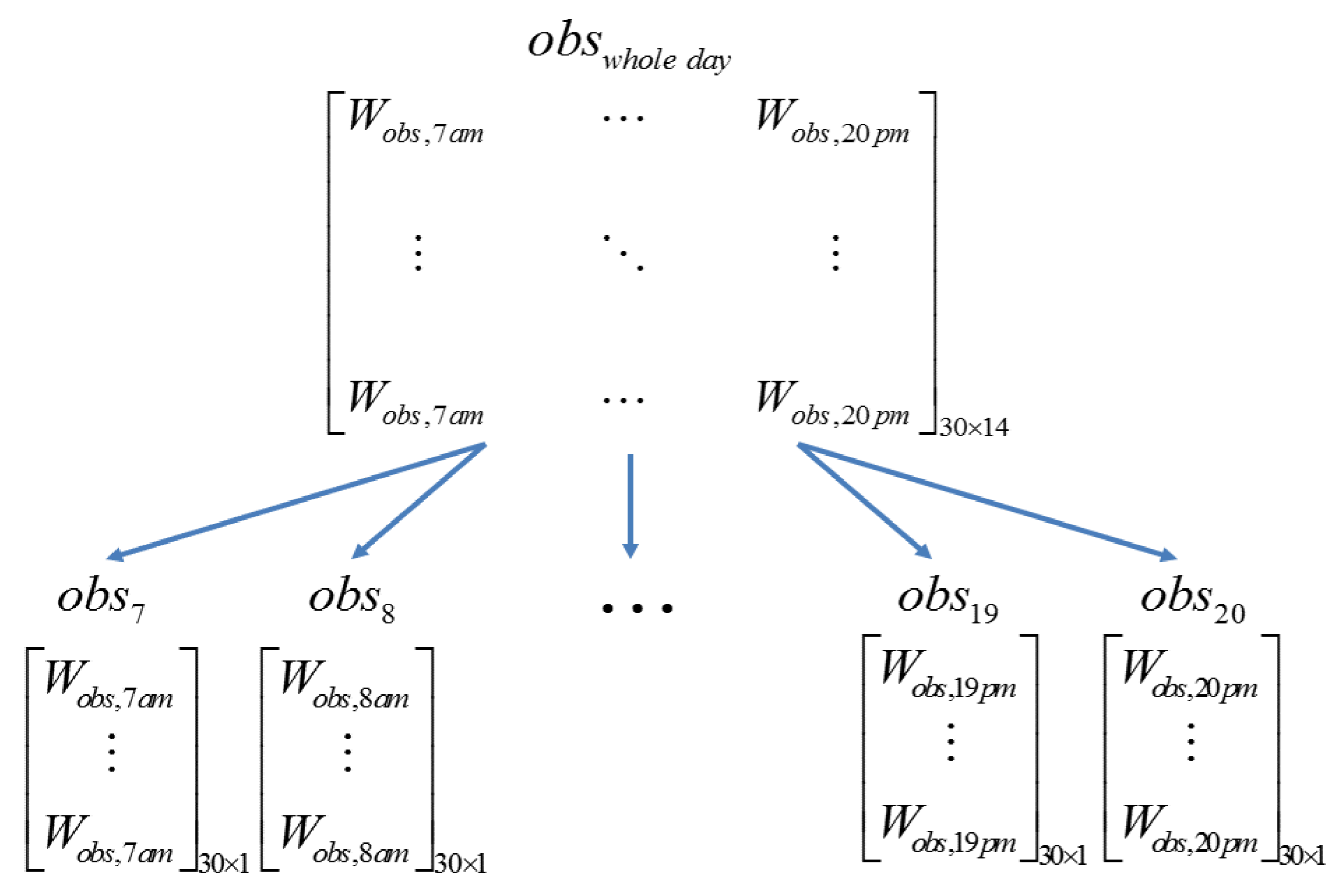
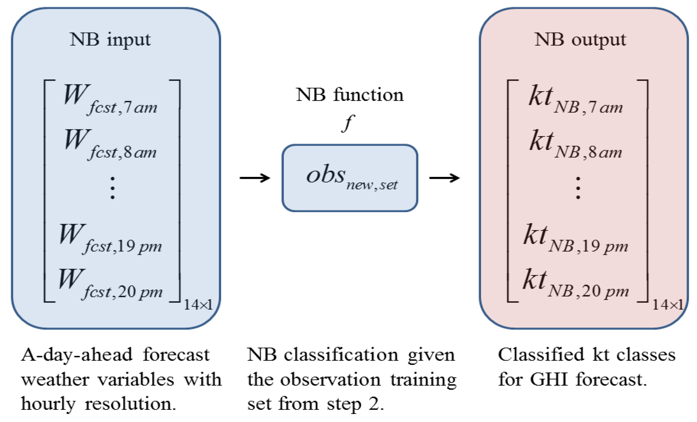
3.3. Step 3: Naïve Bayes Classifier

The naïve Bayes (NB) classifier is an effective probabilistic classification algorithm. Based on the Bayes’ theorem, the NB algorithm performs the classification with the assumption that the features (the weather variables) are independent of each other in a given class (a value of kt). This assumption considerably simplifies the training step of the proposed algorithm for weather forecasting, and, for that reason, the calculations are fast while the performance is highly accurate in many practical applications [16].

Figure 5 represents the NB model process. The input value, in conjunction with the observation training set, draws the output value of $k{t}_{NB}\in \left\{1,\cdots ,100\right\}$ that belongs to each hour in the daytime period. Unlike the observation feature $W_{obs,h}\in {ℝ}^{1\times 4}$ in step 1, the forecasted feature vector $W_{fcst,h}\in {ℝ}^{1\times 3}$, which includes $V_{Temp,h}$, $V_{RH,h}$, and $V_{DP,h}$, is used as input to the proposed NB model. The relationship between input and output in Figure 5 can be expressed as follows:

$$kt\left(h+48\right)=f\left[V_{Temp}\left(h+48\right),V_{RH}\left(h+48\right),V_{DP}\left(h+48\right)\right],$$

(6)

where the function f represents the NB classification.

3.3.1. Estimation of $P(V_i|C)$: Kernel Methods

The estimation of $P(V_i|C)$ requires itself an estimation of the probability density functions (PDF) for the random variables involved. This estimation can be implemented using parametric or non-parametric methods. The parametric estimation for the PDF assumes that it is a member of some parametric family of distributions, e.g., a normal distribution $N\left(\mu ,{\sigma }^2\right)$. When this assumption is correct, the parameters (mean $\mu$ and standard deviation $\sigma$ in case of the Gaussian) can easily be estimated from the data. However, when the underlying distribution generating the data has multiple modes or a skewed shape, the probability calculation might be wrong due to the restrictions imposed by the choice of the distributions family.

Non-parametric kernel density estimation can deal with large variations in the features. In other words, the kernel density estimation does not require the assumption that the features follow some generic probability distribution as mentioned above. In addition, since the GHI classification is a nonlinear problem [17], the kernel density function may be preferable to the estimation of $P(V_i|C)$. Therefore, this paper used the kernel density function based on a Gaussian kernel in order to estimate $P(V_i|C)$. The Gaussian kernel for each feature $V_i$ is given by

$$K_{gau}\left(V_{i,n},{\sigma }_i\right)=\exp \left(\frac{-V_{i,n}{}^2}{2{\sigma }_i{}^2}\right),$$

(7)

where $V_{i,n}$ indicates $n$ observations ($V_{i,1},V_{i,2},\cdots ,V_{i,n}$) and ${\sigma }_i$ represents the bandwidth. The bandwidth has a decisive effect on the decay of the Gaussian kernel in Equation (7). However, the methods used to choose ${\sigma }_i$ are seldom discussed in related works. The bandwidth ${\sigma }_i$ can be determined from an estimator ${\widehat{\sigma }}_i$, which is a combination of the inter-quartile range ${\widehat{R}}_i$ and a rule-of-thumb bandwidth [18]. First, the inter-quartile range ${\widehat{R}}_i$ is determined as

$$\widehat{R_i}=V_{i,Q3}-V_{i,Q1},$$

(8)

which indicates that the interquartile range ${\widehat{R}}_i$ is the length of the interval in the support of the feature $V_i$ between the upper quartile of 75% ($V_{i,Q3}$) and the lower quartile of 25% ($V_{i,Q1}$). Equation (8) can also be transformed into the standardized Z-scale [19], which has a Gaussian with zero mean and a unity standard deviation, as shown in Equation (9) by rescaling the horizontal axis with the feature mean $E\left(V_i\right)$ and the standard deviation $\sigma \left(V_i\right)$

$$Z_i=\frac{V_i-E\left(V_i\right)}{\sigma \left(V_i\right)}.$$

(9)

Based on Equation (9), then, the inter-quartile range ${\widehat{R}}_i$ in Equation (8) can be derived as

$$\begin{gathered} {\widehat{R}}_i=\left(E\left(V_i\right)+\sigma \left(V_i\right)Z_{Q3}\right)-\left(E\left(V_i\right)+\sigma \left(V_i\right)Z_{Q1}\right)=\sigma \left(V_i\right)\left(0.675-\left(-0.675\right)\right) \\ =1.35\sigma \left(V_i\right), \end{gathered}$$

(10)

$$\sigma \left(V_i\right)=\frac{{\widehat{R}}_i}{1.35}.$$

(11)

The standard deviation $\sigma \left(V_i\right)$ in Equation (11) is then plugged into the rule-of-thumb bandwidth ${\widehat{\sigma }}_{i,rot}$ in Equation (12), where n represents the number of hourly values in feature $V_i$:

$${\widehat{\sigma }}_{i,rot}={\left(\frac{4\sigma {\left(V_i\right)}^5}{3n}\right)}^{0.2}\approx 1.06\sigma \left(V_i\right)n^{-0.2},$$

(12)

$${\widehat{\sigma }}_{i,rot}=1.06\frac{{\widehat{R}}_i}{1.35}{n}^{-0.2}.$$

(13)

3.3.2. Update Posterior of C: Calculating the Value of $P(C|V_i)$

Once the bandwidth estimator ${\widehat{\sigma }}_{i,rot}$ in Equation (13) is derived, the above process, Equation (7) through (13), is repeated in the training step in order to estimate a posterior density of each feature in each class using the Gaussian kernel density estimation. Based on the training step, the NB classifier can be expressed as:

$$k{t}_{NB}=\underset{C\in \left\{1,\cdots ,l\right\}}{\arg \max }P\left(C\right){\displaystyle \prod }_{i}P(V_i|C),$$

(14)

where the $k{t}_{NB}$ stands for the target class value, chosen to be the one maximizing the probability in Equation (14). Therefore, this proposed NB model is used to estimate the hourly GHI by multiplying ESR in Equation (3) by $k{t}_{NB}$ from Equation (14). It is worth noticing that the $k{t}_{NB}$ value has interval $\left[\left(l-1\right)\times 0.01;l\times 0.01\right]$, where l = 1, $\cdots$, 100, so the median value of 0.005 is used for the $k{t}_{NB}$ when GHI is re-estimated. Furthermore, after training, two-day-ahead average daily solar energy can be forecasted by summing the daily $k{t}_{NB,h}$ values regardless of the previous forecast results, since the input values are obtained from the weather reports.

4. Forecasting Test

The outputs of the proposed NB model, the kt classes, are re-converted to GHI values to compare with actual GHI. In order to consider seasonal effects, several error tests are compared month-by-month from August 2013 to March 2014.

4.1. Diagnostic Checking

To comprehensively evaluate the forecasting performance clearly, multiple error metrics were calculated. These metrics are the mean bias error (MBE), the mean absolute error (MAE), the root mean square error (RMSE), and the relative mean bias error (RMBE), where the subscript i in Equations (15) to (20) represents the ith forecast and observation pair given the forecasting horizon length. For example, N is equal to 434 (14 daily points $\times$ 31 days) for August. With an hourly resolution, the error evaluations are restricted to the daytime hours (14 points).

Depending on the various purposes, the error criteria can be mutually complementary for analyzing the forecast quality. Usually RMBE (Equation (19)) or MAPE (Equation (20)) are used for forecast testing, but these are often unclear on the normalizing factor (measured mean or maximum value). The MBE (Equation (16)) measures the tendency of solar energy that is over-estimated or under-estimated given the forecasting period. For example, the MBE can be directly used for an evaluation of real application such as PV-energy-storage system. The MAE (Equation (17)) measures an absolute difference that is less biased than the RMSE in Equation (19) in large error cases. Similar to the MSE, the MAPE (Equation (20)) is widely used for forecasting the model performance, but the MAPE is not bounded in case that the errors are greater than the actual value [20]. The RMSE represents the variation between forecasted and actual data that are usually used for short-term forecast (less than one-day). The RMBE (Equation (19)) shows the relative MBE value, which is normalized by the average of GHI within the observation period.

$$E={\mathrm{GHI}}_{fcst,i}-{\mathrm{GHI}}_{obs,i}$$

(15)

$$\mathrm{MBE}=\frac{1}{N}{\displaystyle \sum }_{i=1}^N\left(E\right)$$

(16)

$$\mathrm{MAE}=\frac{1}{N}{\displaystyle \sum }_{i=1}^N|E|$$

(17)

$$\mathrm{RMSE}=\sqrt{\frac{1}{N}{\displaystyle \sum }_{i=1}^N{\left(E\right)}^2}$$

(18)

$$\mathrm{RMBE}=\frac{\mathrm{MBE}}{\frac{1}{N}{{\displaystyle \sum }}_{i=1}^N{\mathrm{GHI}}_{obs,i}}100$$

(19)

$$\mathrm{MAPE}=\frac{1}{N}{\displaystyle \sum }_{i=1}^N\frac{|E|}{{\mathrm{GHI}}_{obs,i}}100$$

(20)

4.2. Model Testing

Before the forecasting results are discussed, it is important to note that summers in Austin have more clear days than during other seasons. Moreover, in order to avoid an infinite result during the computation procedure, the denominator in Equation (20) was replaced by 1 during nighttime, when the GHI result was close to zero.

4.2.1. Monthly Results: Seasonal Effect

Table 1. Summary of Statistical Values for Actual GHI and Two-Day-Ahead Forecast Errors.

Month	$\mathbf{Min}./\mathbf{Max}.(\mathbf{Wh}/{\mathbf{m}}^2)$	$\mathbf{Mean}(\mathbf{Wh}/{\mathbf{m}}^2)$	$\mathbf{Std}.(\mathbf{Wh}/{\mathbf{m}}^2)$	r (%)	Training Days	$\mathbf{MBE}(\mathbf{Wh}/{\mathbf{m}}^2)$	MAE (Wh/m2)	$\mathbf{RMSE}(\mathbf{Wh}/{\mathbf{m}}^2)$	RMBE (%)
August	5/999	551.28	306.65	90.38	26	33.42	62.31	126.8	6.06
September	0/926	452.85	302.79	86.55	26	23.46	78.18	143.64	5.18
October	0/879	348.18	284.98	84.7	28	12.56	84.48	143.66	3.61
November	0/746	227.11	232.94	87.29	36	40.49	76.51	117.22	17.83
December	0/643	210.87	212.16	78.37	40	4.95	73.77	126.49	2.35
January	0/745	273.30	240.28	91.42	50	–11.09	57.04	91.03	–4.06
February	0/853	254.80	269.35	80.98	24	–12.89	105.17	147.91	–5.06
March	0/972	338.68	300.83	80.9	30	–32.85	107.37	167.32	–9.7
Total	0/999	333.04	292.47	86.33	30	9.09	80.39	138.85	2.73
(8 months)

shows a summary of the statistical values relevant to the two-day-ahead GHI forecast. For the actual GHI, the minimum, maximum, mean, and correlation coefficient, $r$, are evaluated month-by-month with hourly resolution. From Table 1, August indicates the maximum GHI and standard deviation with the largest mean of 551.28 Wh/${\mathrm{m}}^2$, while December shows the smallest GHI and standard deviation with the smallest mean of 210.87 Wh/${\mathrm{m}}^2$. Similar to the GHI profile, r, which represents the linear relationship between actual and forecasted values, also shows the maximum of 90.38% for August and minimum of 78.37% for December. The RMBE of August through December indicates an overestimation in the NB model, while the rest of the months show the reverse tendency. Particularly, the MAPE is not evaluated in the monthly analysis (Table 1) because of its unbounded property.

4.2.2. 4-Days-Results: Various Weather vs. Specified Weather Types

Figure 6, Figure 7, Figure 8 and Figure 9 compare the two-day-ahead forecasts and actual GHI values with the various weather types for 4 days. This various weather analysis is similar to the established analytical practices in [9,10] in that test period of 4 days. However, the various weather analysis shows real-time weather change that is not specified with specific weather types (i.e., sunny, cloudy, or rainy). On the days that are clear (5–8 August 2013), Figure 6 and type 1 in

Table 2. Summary of Two-Day-Ahead Forecasted Errors for 4 days.

Weather Type	r (%)	RMBE (%)
Type 1	99.82	−1.49
Type 2	84.16	−1.33
Type 3	96.86	−3.4
Type 4	74.18	−8.43

indicate that the forecasted GHI has a good agreement with the actual GHI.

Figure 7 shows a mix of 2 clear, 1 partly cloudy, and 1 overcast day (10–13 December 2013), where the GHI decreases significantly on the last day. In contrast, the 3 overcast days and 1 clear day (24–27 February 2014) depicted in Figure 8 show that GHI sharply increases on the last day. Though there are some differences between forecasted and actual values on the last day in Figure 7 and Figure 8, the proposed NB model shows that the forecasted GHI follows the actual values. In addition, the following actual tendency can be proved with Table 2. For types 2 and 3, Table 2 indicates that r is 84.16% and 96.86%, respectively, which means that the forecasted values significantly follow the actual GHI trends for four days.

At this point, it is worth comparing the forecasting performance of the proposed NB model (Table 2) against the approach of a previous study (ANN, see Table 3 in [10]) that might be helpful to understand how the proposed NB algorithm follows the real weather change. The previous study in [10] represents three layers (input, hidden, output layer) based on radial basis functions (RBF) and uses six input variables (day of month, solar power, relative humidity, wind speed, solar irradiance, air temperature).

Table 3. Summary of One-Day-Ahead Forecast Errors for 4 days.

Method	Structure	Weather Type	r (%)	RMBE (%)	MAPE (%)
ANN in [10]	Three layers (input, hidden, output) & 6 input variables	Sunny	98.77	x	9.45
		Cloudy	98.46	x	9.88
		Rainy	65.63	x	38.11

(re-produced from [10]) shows an r of 65.63% for rainy days, which is a poorer result than that of type 3 in the NB model (i.e., 96.86%). Though that study could recognize the rainy days’ pattern—lower actual GHI—during 4 rainy days, the recognized pattern could not reflect the actual values’ tendency. Contrary to this, the NB model (type 3) was able to anticipate the tendency of the various weather types for 4 days, which include not only the 3 overcast days but also 1 clear day. Strictly speaking, because of different environment and weather types, the performance of the model in [10] may not be directly comparable with that of the proposed NB model. However, given the test criteria, r, which indicates the linear relationship between the forecasted and actual values, it is reasonable to compare the forecasting performance of the NB model with that of the previous study. Moreover, and more importantly, it can also be said that the proposed NB model has better forecasting performance than the previous one when the forecasting time scale is considered (the proposed NB model of two days vs. the previous study of one day).

Lastly, Figure 9 shows 1 clear and 3 partly cloudy days (25–28 March 2014), which represent the typical GHI variability by cloud movement. From the results (Figure 6, Figure 7, Figure 8 and Figure 9), most of the differences between forecasted and actual values occur on cloudy days.

5. Conclusions

An hourly solar irradiance NB model was developed for two-day-ahead forecast. Publicly available weather observation and forecast data were used as training sets and input values in the model. A key contribution of this paper was to reduce the GHI uncertainty by partitioning daily hourly intervals into subsets and by considering the effect of clouds in training step. Furthermore, the proposed NB model is considerably simple and fast in that it requires small training data (less than two months) and uses only four weather variables (temperature, relative humidity, dew point, and sky coverage). The NB model’s forecast accuracy was demonstrated with statistics values and several error metrics. For an eight-month period with hourly resolution (14 h per day), the proposed NB model provided forecasting results with RMBE of 2.73% and r of 86.33% with a GHI mean of 333.04 Wh/m². For the various weather types, four clear days represent RMBE of—1.49% and an r of 99.85%, which considerably match with the actual GHI. In particular, the proposed NB model showed reasonable results under various weather conditions (types 2, 3, and 4) as the forecasted GHI values tended to follow the actual GHI’s ones.

References

1. Hosenuzzaman, M.; Rahim, N.A.; Selvaraj, J.; Hasanuzzaman, M.; Malek, A.A.; Nahr, A. Global prospects, progress, policies, and environmental impact of solar photovoltaic power generation. Renew. Sustain. Energy Rev. 2015, 41, 284–497. [Google Scholar] [CrossRef]
2. Kamada, R.; Yagioka, T.; Adachi, S.; Handa, A.; Tai, K.F.; Kato, T.; Sugimoto, H. New world record Cu (In, Ga)(Se, S) 2 thin film solar cell efficiency beyond 22%. In Proceedings of the Photovoltaic Specialists Conference (PVSC), Portland, OR, USA, 5–10 June 2016; pp. 1287–1291. [Google Scholar]
3. Bacha, S.; Picault, D.; Burger, B.; Etxeberria-Otadui, I.; Martins, J. Photovoltaics in microgrids: An overview of grid integration and energy management aspects. IEEE Ind. Electron. Mag. 2015, 9, 33–46. [Google Scholar] [CrossRef]
4. Schittekatte, T.; Stadler, M.; Cardoso, G.; Mashayekh, S.; Sankar, N. The impact of short-term stochastic variability in solar irradiance on optimal microgrid design. IEEE Trans. Smart Grid 2018, 9, 1647–1656. [Google Scholar] [CrossRef]
5. Monjoly, S.; Andre, M.; Calif, R.; Soubdhan, T. Hourly forecasting of global solar radiation based on multiscale decomposition methods: A hybrid approach. Energy 2017, 119, 288–298. [Google Scholar] [CrossRef]
6. Masters, G.M. Renewable and Efficient Electric Power Systems; Wiley & Sons: Hoboken, NJ, USA, 2004. [Google Scholar]
7. Raza, M.Q.; Nadarajah, M.; Ekanayake, C. On recent advances in PV output power forecast. Sol. Energy 2016, 136, 125–144. [Google Scholar] [CrossRef]
8. Reikard, G. Predicting solar radiation at high resolutions: A comparison of time series forecasts. Sol. Energy 2009, 83, 342–349. [Google Scholar] [CrossRef]
9. Mellit, A.; Pavan, A.M. A 24-h forecast of solar irradiance using artificial neural network: Application for performance prediction of a grid-connected PV plant at Trieste, Italy. Sol. Energy 2010, 84, 807–821. [Google Scholar] [CrossRef]
10. Chen, C.; Duan, S.; Cai, T.; Liu, B. Online 24-h solar power forecasting based on weather type classification using artificial neural network. Sol. Energy 2011, 85, 2856–2870. [Google Scholar] [CrossRef]
11. Sfetsos, A.; Coonick, A.H. Univariate and Multivariate Forecasting of Hourly Solar Radiation with Artificial Intelligence Techniques. Sol. Energy 2000, 68, 169–178. [Google Scholar] [CrossRef]
12. Kemmoku, Y.; Orita, S.; Nakagawa, S. Daily insolation forecasting using a multi-stage neural network. Sol. Energy 1999, 66, 193–199. [Google Scholar] [CrossRef]
13. NOAA. Available online: http://www.noaa.gov (accessed on 23 March 2019).
14. WeatherSpark. Available online: http://weatherspark.com/averages/29684/Austin-Texas-United-States (accessed on 23 March 2019).
15. Poggi, P.; Notton, G.; Muselli, M.; Louche, A. Stochastic study of hourly total solar radiation in Corsica using a Markov model. Int. J. Climatol. 2000, 20, 1843–1860. [Google Scholar] [CrossRef] [Green Version]
16. Mitchell, T. Machine Learning, 1st ed.; McGraw-Hill Science/Engineering/Math: New York, NY, USA, 1997; ISBN 0070428077. [Google Scholar]
17. Shi, J.; Lee, W.J.; Liu, Y.; Yang, Y.; Peng, W. Forecasting Power Output of Photovoltaic System Based on Weather Classification and Support Vector Machines. IEEE Trans. Ind. Appl. 2012, 48, 1064–1069. [Google Scholar] [CrossRef]
18. Härdle, W. Smoothing Technique: With Implementation in S.; Springer: New York, NY, USA, 1991. [Google Scholar]
19. DeGroo, M.H.; Schervish, M.J. Probability and Statistics; Addison Wesley: Boston, MA, USA, 2001. [Google Scholar]
20. Armstrong, J.S.; Collopy, F. Error Measures for Generalizing about Forecasting Methods: Empirical Comparisons. Int. J. Forecast. 1992, 8, 69–80. [Google Scholar] [CrossRef]
Figure 1. Eight months solar irradiance data set used in naïve Bayes (NB) model: (a) Hourly actual global horizontal irradiance (GHI); (b) normalization factor extraterrestrial solar radiation (ESR); (c) clear index kt.
Energies 12 01529 g001
Figure 2. GHI variation on a clear and an overcast day.
Energies 12 01529 g002
Figure 3. The fourteen-hour observation training sets obtained from the inclusion of the daylight data only (step 1).
Energies 12 01529 g003
Figure 4. Filtered training set using the forecasted sky coverage variable (step 2).
Energies 12 01529 g004
Figure 5. Modified NB classification using forecasted weather variables (step 3).
Energies 12 01529 g005
Figure 6. Comparison between two-days-ahead forecasted and actual GHI for clear 4 days (type 1).
Energies 12 01529 g006
Figure 7. Comparison between two-days-ahead forecasted and actual GHI for 2 clear, 1 partly cloudy, and 1 overcast day (type 2).
Energies 12 01529 g007
Figure 8. Comparison between two-days-ahead forecasted and actual GHI for 3 overcast and 1 clear day (type 3).
Energies 12 01529 g008
Figure 9. Comparison between two-days-ahead forecasted and actual GHI for 1 clear and 3 partly cloudy days (type 4).
Energies 12 01529 g009