Spatiotemporal Correlations in the Power Output of Wind Farms: On the Impact of Atmospheric Stability

Abstract

The dependence of temporal correlations in the power output of wind-turbine pairs on atmospheric stability is explored using theoretical arguments and wind-farm large-eddy simulations. For this purpose, a range of five distinct stability regimes, ranging from weakly stable to moderately convective, were investigated with the same aligned wind-farm layout used among simulations. The coherence spectrum between turbine pairs in each simulation was compared to theoretical predictions. We found with high statistical significance (p < 0.01) that higher levels of atmospheric instability lead to higher coherence between turbines, with wake motions reducing correlations up to 40%. This is attributed to higher dominance of atmospheric motions over wakes in strongly unstable flows. Good agreement resulted with the use of an empirical model for wake-added turbulence to predict the variation of turbine power coherence with ambient turbulence intensity (R${}^2$ = 0.82), though other empirical relations may be applicable. It was shown that improperly accounting for turbine–turbine correlations can substantially impact power variance estimates on the order of a factor of 4.

1. Introduction

The characteristics of spatiotemporal correlations in atmospheric flows play a major role in determining the variability of wind-power resources. For instance, Archer and Jacobson [1] found that interconnecting a number of wind farms would allow for an average of 33% of the yearly averaged power to be used as baseload power by reducing power variability. This occurs due to the fact that distant wind farms are not strongly correlated, whereas a single wind farm is not able to reliably supply baseload power. Using power data from a set of 19 wind farms, Archer and Jacobson [1] suggested that there was seemingly no limit to power-variability reduction via inclusion of more geographically dispersed wind farms. Katzenstein [2] used a dataset from 20 wind farms in Texas to show how geographic smoothing impacted wind-power fluctuations at different timescales. They found that over timescales of one hour, a reduction in power variability of 87% was achieved, while the 24-h variability was not significantly attenuated. This is consistent with the findings of Bandi [3], who used turbulence theory to show that a limiting behavior exists in the smoothing of wind-power fluctuations, and used the same Texas wind-farm dataset as Katzenstein [2] as well as a set of 224 Irish wind farms to confirm that this limit has already been reached in these two aggregates. A similar asymptote in smoothing behavior was found by Fertig et al. [4], who analyzed the power output of a large number of wind farms throughout the United States, considering the effect of theoretical interconnects between four geographical regions (the Bonneville Power Authority in the Northwestern United States, the Electrical Reliability Council of Texas, the Midwest Independent System Operator, and the California Independent System Operator). They found that much of the reduction in variability that was achieved with a very large number of wind plants across regions can be reproduced with only four or five plants within a single region.

It is clear from the literature that correlations corresponding to length scales on the order of hundreds of meters and timescales from an hour to days impact power fluctuations [5]. However, Fertig [4] noted that Sørensen [6] used a similar method of analysis to investigate fluctuations over short timescales in a single wind farm, pointing to a “fractal property of wind energy”. Sørensen [6] noted that the spectrum of the power fluctuations from a wind farm includes cross-spectral terms and modeled them with an empirical coherence function, originally suggested by Schlez and Infield [7], which uses fitted constants to model the decay of correlation at high frequencies as a function of streamwise and lateral displacement, and found that this empirical model fit well to the data from two offshore wind farms in Denmark. Also included in their model coherence function is a complex exponential term that accounts for the phase lag as motions pass between rows of turbines, though the implications of this assumption were not discussed. Over short timescales, when the wind is relatively steady, Stevens and Meneveau [8] observed that strong spectral peaks occur in the aggregate spectrum of a wind farm, and these peaks correspond to the time it takes for turbulent motions to pass from one row of turbines to the next. This is consistent with the suggestion of Sørensen [6] that the coherence spectrum has a sinusoidal characteristic associated with the inter-row passage time scale.

Though Sørensen [6] showed that the empirical coherence function of Schlez and Infield [7] was effective in predicting the correlation terms in the spectra of wind farms, recent effort has gone toward a more physical understanding, using the Kraichnan–Tennekes [9,10] random-sweeping hypothesis (RSH). Liu et al. [11] applied the RSH as part of an effort toward modeling the power fluctuations of an entire wind farm, and arrived at an expression for the coherence function that did not depend on fitted parameters but instead on the turbulence intensity of the incoming boundary-layer flow and showed good agreement with wind–tunnel experiments. Works by Bossuyt et al. [12] and Lukassen et al. [13] similarly used the RSH in treating a wind farm as a discrete sampling kernel of the turbulent boundary layer and successfully predicted the correlation characteristics of wind-tunnel data and large-eddy simulations, respectively.

However, both Liu et al. [11] and Bossuyt et al. [12] made the simplifying assumptions of a wind farm in a near-neutrally stable atmospheric boundary layer and that wakes do not play an important role in determining the correlations of turbine pairs. However, in both instances, the magnitude of the spectral peaks was slightly overestimated, particularly for pairs of turbines that were separated by more than one row. This may be because, depending on the lateral separation between a pair of wind turbines, either turbine may experience wake motions, such as meandering of wake motions [14], from upwind turbines. As wake motions tend to be much smaller in scale than boundary-layer motions and are inherently localized, a component of the turbulence approaching either turbine may, then, not be strongly correlated with that approaching the other turbine. Since the characteristics of the boundary-layer turbulence depend strongly on the atmospheric stability state, the fractional contribution to the overall turbulence kinetic energy that is due to upwind wake motions, and therefore the characteristics of turbine-turbine correlations, should therefore depend on atmospheric stability.

In this paper, we aim to explore the characteristics of the coherence spectrum of turbine pairs as a function of atmospheric stability and wake-added turbulence, with data from large-eddy simulations spanning several atmospheric stability conditions. In Section 3, the methods of performing the large-eddy simulations as well as the details on the different stability states are presented. In Section 4, the impact of flow conditions on turbine-turbine coherence is investigated, as well as the effects of lateral displacement between turbine pairs.

2. Coherence and the Random-Sweeping Hypothesis

The Kraichnan–Tennekes random-sweeping hypothesis is an expansion of the frozen turbulence hypothesis, which makes the assumption that turbulent motions are advected by the mean velocity and do not evolve temporally. The RSH similarly assumes that turbulent motions do not evolve temporally but adds a random-sweeping velocity to the advection, so that:

$$\frac{\partial {\mathbf{u}}^{\prime }}{\partial t}+(\mathbf{V}+{\mathbf{v}}^{\prime })\frac{\partial {\mathbf{u}}^{\prime }}{\partial \mathbf{x}}=0,$$

(1)

where ${\mathbf{u}}^{\prime }$ is the vector field of turbulent fluctuating velocity, $\mathbf{V}$ is the mean velocity vector, and ${\mathbf{v}}^{\prime }$ is a large-scale sweeping velocity. The application of the RSH to spatiotemporal correlations in the atmospheric boundary layer was studied in detail by Wilczek et al. [15]. By assuming that the fluctuating part of the sweeping velocity is zero-mean and normally distributed with standard deviation ${\sigma }_1$, Liu et al. [11] suggested that the cross-spectrum ${\mathsf{\Phi }}_{1,2}$ of the power output of two turbines spaced a distance $\Delta x$ apart in the direction of the mean flow such that the lateral component of the mean velocity is zero, would take the form:

$${\mathsf{\Phi }}_{1,2}(f)=\sqrt{{\mathsf{\Phi }}_{1,1}{\mathsf{\Phi }}_{2,2}}\exp \left(-\frac{2\pi if\Delta x}{U}\right)\times \exp \left(-\frac{2{\pi }^2{f}^2\Delta x^2{\sigma }_1^2}{3U^4}\right),$$

(2)

and therefore, the coherence spectrum $C_{1,2}$, a nondimensional quantity which describes the correlation of two time series across frequency scales, could be expressed as:

$$\begin{array}{cc}\hfill C_{1,2}(f)=& \frac{{\mathsf{\Phi }}_{1,2}}{\sqrt{{\mathsf{\Phi }}_{1,1}{\mathsf{\Phi }}_{2,2}}}=\exp \left(-\frac{2\pi if\Delta x}{U}\right)\times \exp \left(-\frac{2{\pi }^2{f}^2\Delta x^2{\sigma }_1^2}{3U^4}\right).\hfill \end{array}$$

(3)

For an in-depth discussion of the derivation of these results, see Section 3.D of Liu et al. [11]. Note, however, that this equation is slightly different than the one derived in Liu et al. [11], where ${\mathsf{\Phi }}_{1,1}$ is used instead of $\sqrt{{\mathsf{\Phi }}_{1,1}{\mathsf{\Phi }}_{2,2}}$. This is due to the assumption made in Liu et al. [11] of homogeneous flow, which the current work does not assume. However, as seen in Figure 7 of Liu et al. [11] and Figures 5 and 6 of Bossuyt et al. [12], a straightforward application of the RSH, treating turbines as probes of turbulence, tends to overpredict the magnitude of the spectral bumps. It should be noted that the term coherence in this manuscript refers specifically to the coherence spectrum of turbine pairs, and not necessarily the presence of coherent motions in the flow, such as wake meandering.

3. Large-Eddy Simulations

We used large-eddy simulation (LES) to simulate a wind farm within the Earth’s atmospheric boundary layer using a finite-volume solver for the incompressible filtered Navier–Stokes equations. The solver contains in-house modifications to the National Renewable Energy Laboratory’s simulator for wind farm applications (SOWFA) [16,17,18] solver for atmospheric turbulence, adding the Moeng surface stress model [19,20] for better capturing the velocity gradient near the wall and the Smagorinsky sub-filter model [21] to SOWFA’s OpenFOAM [22] framework.

The velocity, $u_i$, is decomposed into the resolved, ${\overline{u}}_i$, and sub-filter, $u_i^{\prime }$, velocities:

$${\overline{u}}_i=u_i-u_i^{\prime },$$

(4)

where the resolved portion is used in the momentum equation:

$$\frac{\partial {\overline{u}}_i}{\partial t}+\frac{\partial }{\partial x_j}({\overline{u}}_i{\overline{u}}_j)=-2{ϵ}_{i3k}{\omega }_3{\overline{u}}_k-\frac{1}{{\rho }_0}\frac{\partial p_0}{\partial x_i}-\frac{1}{{\rho }_0}\frac{\partial \tilde{p}}{\partial x_i}-\frac{\partial {\tau }_{ij}^D}{\partial x_j}+g\left(\frac{\overline{\theta }-{\theta }_0}{{\theta }_0}\right)+\frac{F_i}{{\rho }_0}.$$

(5)

It is solved with the Coriolis force due to the Earth’s rotation, ${\omega }_3$, with the sign found using the Levi–Civita permutation, $ϵ$, with the 3 indicating vertical direction, the driving pressure gradient using $p_0$ to set the mean wind speed, the local pressure gradient, $\tilde{p}$, the viscous stresses, $\tau$, and the Boussinesq approximation for the buoyancy taking into account the local temperature variation using the potential temperature, $\theta$, and gravity, g, along with the force due to the wind turbine, $F_i$. We used second-order schemes for spatial and temporal derivatives as suggested by Churchfield et al. [16], and the precursor-to-wind farm one-way coupling documented by Churchfield et al. [16] and Jha et al. [23]; this allows for developing atmospheric turbulence in a larger, periodic domain, which is then fed into a smaller domain with the wind farm, where the turbine wakes can develop and interact with other turbines.

A 5 km × 5 km × 2 km precursor domain with 10 m spacing was used to develop atmospheric turbulence, with a periodic inflow boundary, and periodic lateral boundaries [24]. The boundary layer is allowed to develop until it reaches equilibrium, where the boundary layer height becomes stationary within a single vertical cell and the friction speed, ${\overline{u}}_{*}={({\overline{\tau }}_w/\rho )}^{1/2}$, becomes constant. This is done with a capping inversion for the moderately-convective and neutral simulations, with heights shown in

Table 1. Atmospheric stability states used for the wind farm simulations.

Boundary Layer	Stability ($-{\mathit{z}}_{\mathit{i}}{\mathit{L}}^{-1}$)	Surf. Heating (K m s${}^{-1}$)	Wind Speed (m s${}^{-1}$)	Turb. Int. (%)	Height (m)
Moderately Convective	7.8	0.20	9.59	17.2	1200
Weakly Convective	2.3	0.04	9.51	15.4	1140
Neutral	0	0	8.41	11.1	990
Weakly Stable	−2.1	−0.03	9.26	8.8	380

through an iterative process changing the pressure gradient for the velocity, the potential temperature inversion, and the surface heating. This process allows for various stability states to be reached with control over the velocity. The turbulence is then fed into a smaller atmospheric boundary layer domain as a temporal boundary condition with mesh resolution of 4 m over a 1.5 km × 1.5 km × 0.4 km domain containing a wind farm with sixteen 2.5 MW turbines modeled using an actuator disk [25] approach, following validated practices [26,27]. The wind turbines are aligned in a 4×4 pattern with 5 rotor diameter (D = 90 m) spacing in both directions ($S_x/D=S_y/D=5$) with the incoming mean wind aligned with the turbine columns. The values for the individual turbine axial induction factors denoted by a are set using the ’none’ SOWFA option, calculating as if turbine pitch and RPM controllers are set to constant values appropriate for the local mean wind speed within the wind farm configuration. A temporally constant geostrophic wind [28] is prescribed to model the low-level jet for the stable boundary layer for the wind-farm simulation. The wind farms are run through the start-up transient where the turbine wakes develop, and then data are sampled for 2000 s.

Table 1 shows the various stability states modeled with the kinematic surface heat flux used as well as the mean wind speed and turbulence intensity, defined as:

$$I_u=\frac{u}{U},$$

(6)

at half the boundary layer height from the precursor simulation. The stability state is characterized by the ratio of scales $\frac{-z_i}{L}$, where $z_i$ is the boundary layer depth and L is the Monin–Obukhov length scale, defined as:

$$L=-\frac{u_{*}^3{\theta }_0}{\kappa g{Q}_0},$$

(7)

where $u_{*}$ is the streamwise friction velocity, ${\theta }_0$ is the potential temperature, $Q_0$ is the kinematic surface flux, g is the gravity, and $\kappa$ is the von Kármán constant. This is also the ratio of the shear and buoyant turbulent energy production. It should be noted that this definition of stability differs from that of Pasquill [29], which is used in, for instance, atmospheric dispersion [30]. The Pasquill definition uses a representative wind speed at a height of 10 m and does not permit either stable or unstable regimes at wind speeds greater than 4 m s${}^{-1}$. 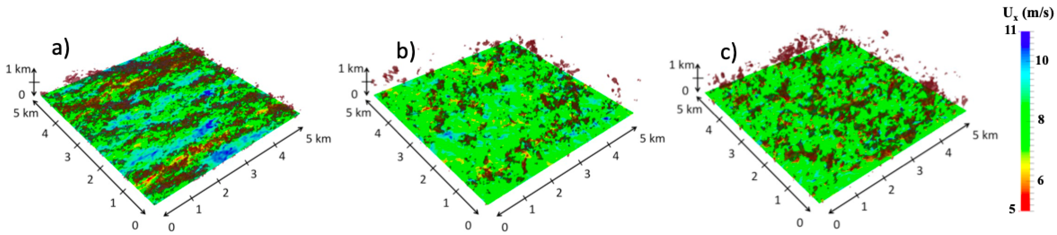While the 10-m wind speeds in the presented simulations are close to this threshold, we proceed by acknowledging that our simulations may not fit the Pasquill definition of stable or unstable boundary layers but are still consistent with stability definitions used in the wind-energy literature. Representative, spatially-distributed instants of the boundary layers at the turbine hub-height are illustrated in Figure 1, where iso-contours of the vertical velocity $u_z=-1$ m s${}^{-1}$ are superimposed for the lower half of the domain. The moderately-convective boundary layer, shown in Figure 1a, has elongated horizontal velocity structures aligned with the flow that correlate well with negative vertical velocity. These structures are on the order of the rotor diameter in width and longer in length, leading to the structure being felt by downwind turbines within the array. The velocity structures in the neutral case (Figure 1b) are smaller than the convective case and are not elongated in the streamwise direction. These structures are on the order of a rotor diameter in both horizontal directions. The weakly stable case illustrated in Figure 1c also lacks the elongated structures found in the moderately-convective case and has structures associated with the temperature gradient not found within the neutral case.

4. Results and Discussion

In calculating the coherence of turbine pairs from the LES, an efficient use of the data is necessary due to the high computational cost. A significant trade off is in maintaining both high frequency resolution at low frequencies and low bias at high frequencies. This trade off lies in the number of sub-windows to use when calculating the spectra and cross-spectra of power output. When using a small number of windows, high-frequency coherence estimates are noisy and biased; however, low-frequency components are estimated with adequate resolution to characterize the advection time. That is, the coherence was estimated at a sufficient number of frequencies to properly characterize a cycle in the advective term of the RSH coherence Equation (3). By contrast, with a large number of windows, the high-frequency coherence results are unbiased, but the low-frequency coherence is not sufficiently resolved. We therefore estimated the coherence with a different number of windows and accepted only a specific range of frequencies from each estimate so that coherence estimates were reported only for frequencies with fewer than 16 cycles in each window, as we found that this gave the best coherence results. The frequency ranges and the number of windows used in that range are listed in

Table 2. Windows used in calculating coherence from large-eddy simulation (LES) data across frequencies.

${\mathit{fS}}_{\mathit{x}}/\mathit{U}$	0–1	1–2	2–4	4–8	8–16	16–32	32–64	64–128
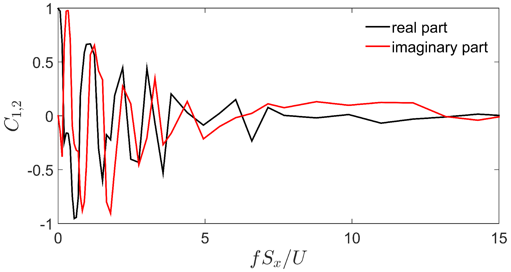
No of windows	2	4	8	16	32	64	128	256

. An example of the calculated coherence from the neutral stability case is shown in Figure 2.

With the coherence estimates, the values of $f_a$ (advection frequency), $f_c$ (decoherence frequency), and $C_0$ (coherence scaling factor) were found such that the RSH estimate minimized the squared error between prediction and data, so that the function fitted to the data was:

$$C_{fit}=C_0\exp \left(-\frac{2\pi if}{f_a}\right)\exp \left(-\frac{f^2}{2f_c^2}\right).$$

(8)

Therefore, $C_{fit}$ is the idealized RSH coherence spectrum that is measured from the data. The two characteristic frequencies $f_a$ and $f_c$ [11] were compared to their prediction from the RSH, namely:

$$f_a=\frac{U}{\Delta x},$$

(9)

which is the inverse of the time it takes to travel between rows of turbines, and:

$$f_c=\frac{U^2}{2\pi \Delta x{\sigma }_1},$$

(10)

which is a characteristic frequency at which turbulent motions between points become uncorrelated, where ${\sigma }_1$ is the rms axial velocity. Further, the dependence of the coherence scaling factor on the turbulence intensity $C_0$ was assessed.

4.1. Advection of Turbulent Motions

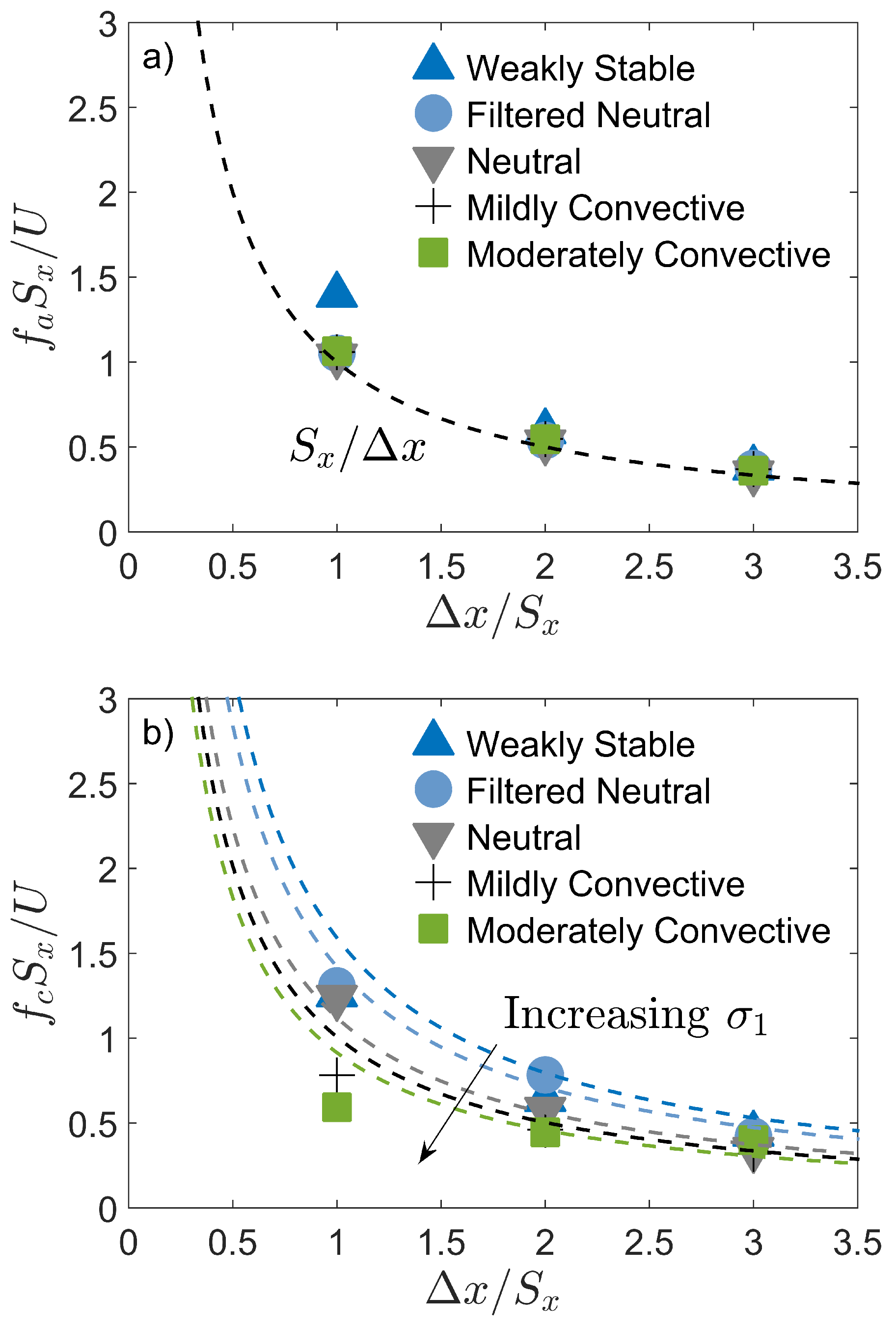
The mean fitted values of $f_a$ are shown in Figure 3a plotted against streamwise distance for each interturbine spacing and for each stability condition. Also included in the figure is the value of $f_a$ predicted by the RSH; it shows a clear trend toward lower frequencies with higher separation, as the advection time between turbines becomes higher. The $f_a$ values fit closely between the five flow conditions. The advection frequency does not appear to be strongly impacted by turbine wakes, at least in the four rows of turbines investigated. This suggests that coherent motions are primarily advected at the boundary-layer velocity rather than the local wake velocity.

The fact that motions are advected at the undisturbed boundary-layer velocity comes with interesting implications about the role of wakes as compared to large-scale atmospheric motions in the context of the RSH. The RSH makes the assumption that the sweeping velocity occurs at length and time scales that are very large compared to turbulence scales of interest. This is a valid assumption for large-scale atmospheric motions, which may be kilometers long and last over timescales on the order of tens of minutes, as compared to typical ∼1 km interturbine separations in wind farms, and the resultant advection time of ∼60 s. However, this is not true for wake-added turbulent motions, which are typically over timescales an order of magnitude higher than the time it takes for the rotor to complete one revolution and smaller [31,32], so that the wake-added motions are similar or smaller in scale to the advection time scale, allowing them to nonlinearly interact. Wake-added motions may then not be expected to contribute to the coherence between turbine pairs, with the coherence instead being dominated by the impinging of turbulent motions from above. Although the added drag by wind turbines will impact the characteristics of the overhead boundary layer, this typically occurs over many rows of turbines and would not be expected to occur over the relatively small extent of the modeled wind farms.

It is noted that no dependence of the lateral spacing on the advective frequency was found; $f_a$ values for turbine pairs that were separated laterally were the same as those not laterally separated within uncertainty.

4.2. Decoherence of Turbulent Motions

Further evidence of the dominant role of atmospheric motions on turbine–turbine correlations is seen in the decoherence frequency, the estimates of which are presented in Figure 3b. The mean values of the decoherence frequency are shown plotted along with their predicted trend, according to Equation (10). The fact that the decoherence frequency follows the trend predicted by the RSH suggests that the proper turbulence intensity scale for this quantity is that of the incoming boundary layer. If the wake turbulence were dominant in the distortion of high-frequency components, a trend should exist showing $f_c$ values deviating below their RSH predictions with larger $\Delta x$, as the wakes of an increasing number of turbines impact the turbulence approaching the downwind turbine in a pair with larger separation. This trend, however, is not observed; though deviations between measurements and RSH predictions are larger than for the values of $f_a$, the boundary-layer turbulence appears to be the appropriate scale in predicting $f_c$.

4.3. Coherence Scaling Factor

Though the timescales of turbine–turbine coherence do not appear to be altered by turbine wakes, the wakes will nonetheless introduce turbulence scales that impact the downwind turbine in a pair and lead to fluctuations in that turbine. Although correlations have been observed between a turbine’s power and the motions in its wake [33], we proceeded with the assumption that these scales are small enough that they experience sufficient nonlinear evolution and do not lead to correlations between the power output of two turbines. There is therefore a fraction of the turbulence approaching the downwind turbine that does not lead to power coherence. This is supported by the strong evidence that turbine–turbine correlation is altered by the turbulence intensity of the upwind turbine of a pair (p < 0.01). Observed correlation values are found to decrease by up to 40% depending on the turbulence characteristics. We proceeded to link this fraction to the wake-added turbulence, using existing empirical formulations from the literature.

The turbulence intensity in the wake, $I_{wake}$, is commonly decomposed [34] into a contribution from the ambient ($I_0$) and wake-added ($I_{+}$) components, as:

$$I_{wake}^2=I_0^2+I_{+}^2.$$

(11)

Since the power spectral density of a turbine’s power output is proportional to the turbulence kinetic energy [35], the coherence should then scale as the Pearson’s correlation coefficient, which in the case of the turbulence intensity can be written as:

$$C_{1,2}\propto \frac{{\widehat{I}}_0{\widehat{I}}_{wake}}{I_0{I}_{wake}},$$

(12)

where ${\widehat{I}}_0$ and ${\widehat{I}}_{wake}$ are the components of the upwind and wake turbulence that are correlated. If the upwind turbulence is assumed to advect naturally between rows via impinging of large-scale motions, and the wake-added turbulence is neglected from turbine-turbine power correlations, then ${\widehat{I}}_0={\widehat{I}}_{wake}=I_0$, and:

$$C_{1,2}\propto \frac{I_0}{\sqrt{I_0^2+I_{+}^2}},$$

(13)

which is a natural prediction for the coherence scaling factor $C_0$. Though the turbulence of the incoming boundary layers was measured during the simulations, the turbulence approaching each turbine was not. We therefore relied on the empirical formulation of Crespo and Hernandez [36] for the wake-added turbulence:

$$I_{+}=0.73a^{0.8325}{I}_0^{0.0325}{(x/d)}^{-0.32},$$

(14)

to predict the turbulence intensity approaching each row of turbines in the five stability cases. We then modeled the coherence scaling factor $C_0^{i,j}$ for turbines i and j as:

$$C_0^{i,j}=\frac{I_i}{I_j},$$

(15)

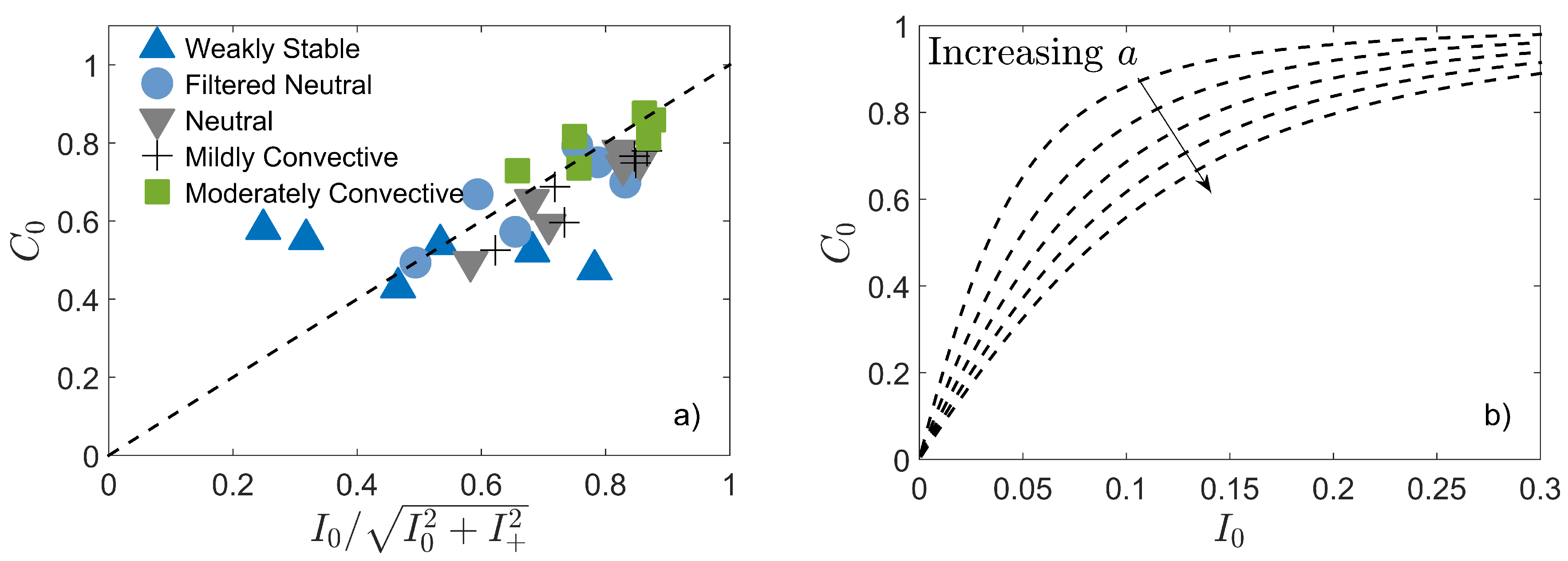
where turbine i is assumed to be farther upwind. The measured values of $C_0$ for turbine pairs that have no lateral separation are depicted in Figure 4a, showing good agreement ($R^2$ = 0.82) with predictions. Although the similarity of layout among the five cases allows for direct testing of the change in coherence scaling factor between flow cases, the noise in these measurements does not allow for a statistically significant trend to be shown toward higher coherence with larger atmospheric turbulence. However, the clear trend in Figure 4a suggests the following approximate functional dependence of the coherence scaling factor on boundary-layer turbulence intensity:

$$C_0=\frac{I_0}{{\left(I_0^2+{(0.73a^{0.8325}{I}_0^{0.0325}{(x/d)}^{-0.32})}^2\right)}^{1/2}}.$$

(16)

This dependence is shown plotted for a pair of turbines separated by 5 rotor diameters for several axial induction factors, from 0.1 to 0.3, over a range of turbulence intensity values in Figure 4b. Although the turbulence model of Crespo and Hernandez [36] adequately predicts the coherence scaling factor, it should be noted that other wake-added turbulence models are commonly used in the literature as well.

4.4. Aggregate Spectrum Modeling

With the modeling approach outlined in the previous sections, it is possible to accurately predict the cross-spectral terms for the power output in a wind farm. The aggregate power spectrum ${\mathsf{\Phi }}_a$ of any N signals takes the form:

$${\mathsf{\Phi }}_a=\sum _{i=1}^N{\mathsf{\Phi }}_{i,i}+2\sum _{i=1}^{N-1}\sum _{j=i+1}^N\Re (C_{i,j}){({\mathsf{\Phi }}_{i,i}{\mathsf{\Phi }}_{j,j})}^{1/2}.$$

(17)

In the case of a wind farm modeled according to the RSH, $C_{i,j}$, the coherence between turbines i and j, is modeled as:

$$C_{i,j}=C_0^{i,j}\exp \left(-\frac{2\pi if\Delta x}{U}\right)\exp \left(-\frac{2{\pi }^2{f}^2\Delta x^2{\sigma }_1^2}{3U^4}\right).$$

(18)

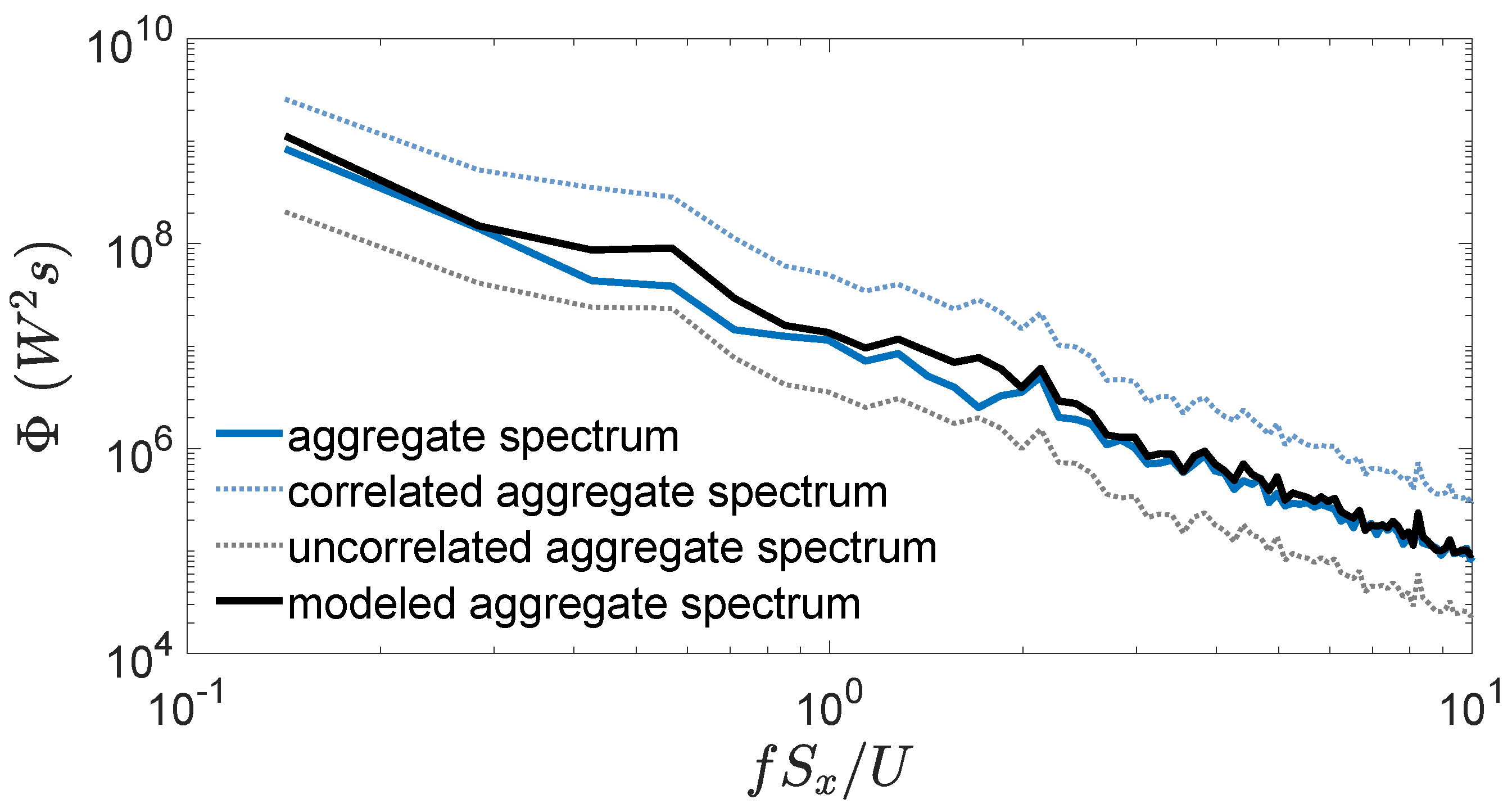
An example of the results of this modeling is shown in Figure 5, which depicts the aggregate spectrum of the neutral boundary-layer case, along with three distinct modeling approaches for the cross-spectral terms in Equation (17). The first approach assumes that $C_{i,j}(f)=1$, equivalent to stating that power fluctuations from all turbines are perfectly correlated with no phase lag. The second approach assumes that $C_{i,j}=0$, or that turbine pairs exhibit no correlation over any time lag. Finally, the third approach applies the RSH-based coherence-modeling methodology outlined above.

It is clear from Figure 5 that proper modeling of cross-spectral terms is an important step in predicting wind-farm variability statistics and that the RSH-based model adequately models these terms. Whereas the variance predicted from the integral of the perfectly correlated aggregate spectrum is overestimated by a factor of approximately 4.0, the variance from the uncorrelated aggregate spectrum is underestimated by a factor of 3.2. However, the variance of the RSH-based model spectrum is overestimated by a much more modest factor of 1.4.

5. Conclusions

Large-eddy simulations were used to show the impact of atmospheric stability on turbine–turbine power coherence. By fitting the data to a predicted coherence function based on the random-sweeping hypothesis, characteristic time scales relating to advection and turbulent decorrelation were deduced and compared favorably with the data, and deviations from the RSH predictions were attributed to wake motions. Results suggest that turbine–turbine power correlations can be largely attributed to large-scale atmospheric motions and that wake-added turbulence does not lead to correlations between turbines, as the reduction in the idealized RSH coherence frequency appears to be a strong function of the wake-added turbulence. This result was used to create an empirical prediction based on the work of Crespo and Hernandez [36] between the ambient atmospheric turbulence and the axial induction factor and spacing of the turbines. This empirical relation fits well with the LES data, suggesting that the dependence of power coherence on the atmospheric stability is primarily a matter of turbulence intensity. However, it should be stated that the fit between the data and the empirical prediction depends strongly on the validity of the existing empirical wake-added turbulence model and that an evaluation of different models may be warranted. When predicting the aggregate power variance of a wind farm, properly modeling turbine–turbine correlations has been shown to be integral.