Urban Wind Resource Assessment: A Case Study on Cape Town

Abstract

As the demand for renewable energy sources energy grows worldwide, small-scale urban wind energy (UWE) has drawn attention as having the potential to significantly contribute to urban electricity demand with environmental and socio-economic benefits. However, there is currently a lack of academic research surrounding realizable UWE potential, especially in the South African context. This study used high-resolution annual wind speed measurements from six locations spanning Cape Town to quantify and analyze the city’s UWE potential. Two-parameter Weibull distributions were constructed for each location, and the annual energy production (AEP) was calculated considering the power curves of four commonly used small-scale wind turbines (SWTs). The two Horizontal Axis Wind Turbines (HAWTs) showed higher AEP and capacity factors than Vertical Axis Wind Turbine (VAWT) ones. A diurnal analysis showed that, during summer, an SWT generates the majority of its electricity during the day, which resembles the typical South African electricity demand profile. However, during winter, the electricity is mainly generated in the early hours of the morning, which does not coincide with the typical load demand profile. Finally, the calculation of Levelized Cost of Electricity (LCOE) showed that SWT generation is more expensive, given current electricity market conditions and SWT technology. The study provides a detailed, large-scale and complete assessment of UWE resources of Cape Town, South Africa, the first of its kind at the time of this work.

1. Introduction

It has been well established that many advantages are associated with harnessing urban wind energy, including climate change mitigation, reduction of transmission losses, and increasing grid reliability, in addition to positive social impacts [1].

Traditional large-scale wind turbines are built with elevated hub-heights to harness wind outside the highly turbulent region of the atmospheric boundary layer, which is closer to the ground and known as the roughness height. The roughness height increases in the presence of rough terrain or obstacles (e.g., trees or buildings) and is a region with highly turbulent and complex flow regimes that are challenging to predict [2,3].

Unlike their large-scale counterparts, small-scale turbines exist in proximity to the ground or buildings and are thus, by nature, present within this complex roughness height region. Urban environments are even more challenging, given the complex flow regime associated with the dense presence of structures, which further intensifies complex turbulent wind flow [4].

Accurate and reliable wind resource assessment is a crucial task before installing generation devices. The single most critical variable in determining wind power potential is the wind velocity vector (incident wind speed and direction relative to the turbine) [5], which, for a given site, can be estimated either by using numerical simulations or real-life measurements.

Turbulent wind flows, which are predominant in the urban environment, are very complex to model mathematically because a closed-form solution of the Navier–Stokes equations does not yet exist. This is more so the case with urban areas, which add even greater complexity due to pervasive wind flow distortion effects of buildings with different geometries, materials, and surface roughness, in addition to varying temperature zones in urban environments. Moreover, the constant variance in wind flow due to naturally dynamic and constantly changing elements of the urban environment makes simulating the wind flow a computationally near-impossible task [6,7,8]. As such, while urban wind measurement and analysis is a challenging task, it is a practical and essential means of reliably quantifying resources before proceeding with installing generation units to reliably exploit wind energy potential in an urban area [1,4].

This study assessed the wind energy potential in the City of Cape Town and is the first large-scale urban wind resource mapping study to be performed for South Africa. Using wind measurements obtained from five different sites spanning Cape Town over a period of two years, 2015 and 2016, a computational analysis was performed to analyze the wind resource potential across the various locations. The annual energy production (AEP) corresponding to different commonly used small-scale wind turbines (SWTs) was calculated for the different sites across the city, and the economic viability of urban wind energy for this case study was assessed.

This manuscript is organized into five sections: Section 1 presents a background and review on small-scale wind power, measurement, and the analysis thereof. Section 2 provides in detail the wind measurement, data collection, and analysis procedures used in this study. In Section 3, the results obtained from station measurements and the proposed methodology for data analysis are provided, first in a step-by-step demonstration on one of the stations, followed by the final results of expected generation capacity and cost of electricity at all stations spanning the city. Then, a discussion of the results is presented in Section 4. Section 5 summarizes the main conclusions of this work.

1.1. Current Status of Urban Wind Energy

A recent report by the World Wind Energy Association (WWEA) states that by 2013 there were at least 870,000 SWTs installed globally with the sector growing significantly between 2005 and 2013, especially in Chinese and American markets [9]. Processes and methods have been streamlined as the urban wind energy sector have grown and matured in these markets.

While the urban wind energy market has grown in other countries, very little information on the potential market exists in South Africa, apart from an initial feasibility study on the installation of a wind turbine in Cape Town [10]. According to the conducted literature review, the current study was the first large-scale urban wind resource mapping study performed in South Africa.

While benefits of installing urban wind turbines are a well-established fact and have been described by many studies [1,11,12,13], there is some work that attempts to identify possible shortcomings of urban wind energy. One study in 2016 considered six urban wind installations in the US and found that the actual electricity production of the turbines was much lower than what was predicted by the project developers in all six [14].

Another study conducted by the Energy Savings Trust used on-site measurement of 57 domestic wind turbines throughout the United Kingdom and found that building-mounted turbines failed to reach load factors of 3% and, in a few cases, the wind turbines were a net user of electricity due to the electricity usage of the inverter [15].

Both studies highlight the need to conduct high-quality wind resource assessment in the design phase of projects, before SWT deployment. The risks of inaccurate wind assessment are not only confined to economic risks, but those risks associated with operating wind turbines should also be considered, including the risk of failure of turbine parts which may lead to human injuries and destruction apart from economic losses.

According to the International Electrotechnical Commission (IEC) 61400-2 standard [16], small-scale wind turbines are defined as turbines whose swept rotor area is smaller than 200 m² and whose rated power is below 50 kW. As such, the wind turbine models assumed in this study (to estimate AEP) had a rated power ranging 800–2500 W, as detailed in Section 2.2.

1.2. Weibull Probability Distributions

The use of probabilistic analysis by means of constructing probability distribution functions (especially Weibull and Rayleigh distributions) from historical wind speed measurements is standard practice when it comes to estimating the potential energy output of a chosen location [17,18,19]. In this study, the two-parameter Weibull distribution was used, which is widely recognized as the most appropriate model in the wind power industry [20]. The Weibull probability density function (PDF) can be calculated as follows:

$$p\left(v\right)=\left(\frac{k}{c}\right){\left(\frac{v}{c}\right)}^{k-1}{e}^{-{\left(\frac{v}{c}\right)}^k}$$

(1)

Accordingly, the cumulative distribution function (CDF) is given by:

$$F\left(v\right)=1-e^{-{\left(\frac{v}{c}\right)}^k}$$

(2)

In Equations (1) and (2), v is the magnitude of wind speed (m/s). The shape of the distribution curve can be altered using the dimensionless shape factor k and scaled using the scaling factor c (m/s). The tuning of the Weibull PDF and CDF using the two parameters was performed based on the measured wind speed data, upon which the probability curves were constructed. The Weibull parameters calculated for each station are listed in

Table 1. Details of wind measurement stations spanning Cape Town, South Africa.

Station Name	Location	Coordinates	Height Above Ground Level (m)	Data Logged (% out of 731 days)	Weibull Shape Parameter (k)	Weibull Scale Parameter (c)	Local Climate Zone Indicator
RCYC	Table Bay Harbor	33°55′13.7″S 18°26′35.0″E	12.1 m	99.8%	1.1	3.7	G
AO	Observatory	33°56′03.6″S 18°28′40.2″E	9.1 m	99.2%	1.8	2.6	9
KBG	Kirstenbosch	33°59′14.9″S 18°25′57.0″E	11.1 m	100%	2.2	2.3	6
MR	Oranjezicht	33°56′18.5″S 18°24′44.0″E	9.4 m	100.0%	1.5	2.6	6
AWS	Airport	33°58′44.0″S 18°36′00.0″E	9.8 m	99.8%	1.9	4.3	D
CTWO	Airport	33°57′46.8″S 18°36′07.2″E	9.3 m	99.8%	1.8	5.7	D

.

It is worth noting that there several other PDFs used in previous studies to estimate wind energy output. As mentioned, the Weibull distribution was selected due to its wide recognition. Several characteristics that have allowed it to become the dominant PDF used in the wind power industry and research field: flexibility, relying on only two parameters, simplicity of parameter estimation, and, being expressed in closed-form, it performs well on goodness-of-fitness tests when parameters are estimated from historical wind speeds. [21]

However, there are certain conditions for which the two-parameter Weibull is not suitable. These include cases with a high number of missing samples, or when the dataset has a bimodal nature. In these cases, an alternative PDF, the Weibull mixture distribution, is recommended. This is a mixture between Weibull and a normal truncated distributions and is especially useful for bimodal samples [21]. Given that all the sample datasets in this study are unimodal, the two-parameter Weibull distribution was confirmed to be appropriate for this study.

1.3. Impact of Urban Environment of Wind Flow

The anemometer heights at all six locations used in for this study are within the Urban Boundary Layer (UBL), which is highly complex and near impossible to model with high accuracy, even relative to the ABL. Within the UBL, the Roughness Sub-layer (RSL) extends up to 2–5 times the average height of existing structures. Inside the RSL, turbulent flow dominates the wind regime, which becomes highly dependent on the surrounding spatial environment [22].

All measurement stations in this study were confirmed to be inside the RSL by investigating their locations. Urban environments are characterized by heterogeneous zones (e.g., size and distribution of buildings and other phenomena such as the urban heat island effect), which contribute further to wind regime complexity. The heterogeneity of urban built environments led to the creation of several classification systems, which aim to present a common assessment framework of urban sites. Those frameworks are generalized and cannot completely account quantitatively for all specific topologies in urban settings. However, they are useful in categorizing different sites qualitatively to provide a comparative framework between different studies and experiments. In this study, the Local Climate Zone (LCZ) framework was chosen to categorize the measurement sites used into 17 different possible categories for urban environments. [23] The LCZ of each station is indicated in Table 1.

2. Methodology

The urban wind resource assessment of Cape Town was performed by means of the following proposed methodology, summarized in the following steps:

• Wind Measurements:   Wind speed measurements from the South African Weather Service.
• Data Pre-Processing: Sorting and transforming data into necessary formats (using Excel).
• Data Analysis:      Analyze wind resource potential (adapted from “bReeze” [24]).
• Calculating AEPs:   Combine wind resource results with SWT power curves to obtain AEP.

Data analysis in this work was performed using an R script, which was written as an adaptation of the “bReeze” open-source package developed by Christian Graul and Carsten Poppinga [24]. bReeze applies a set number of functions to wind data in order to calculate the wind energy resource potential of a specific location.

This study used a statistical approach to infer the characteristics of the surrounding wind regime from historical field measurements. Recently, there has been an increase in the use of computational simulations, which was driven by the significant improvement of computational resources. The two most common simulation approaches are Energy Balance Models (EBM) and Computational Fluid Dynamics (CFD) models. The main advantage of the numerical simulations was the ability to simulate different scenarios in addition to providing information on a wide variety of variables anywhere within the computational domain as opposed to observational models, which rely on a fixed number of recording points. CFD models are especially useful in urban wind energy assessments, as they can study the effects of wind speeds, temperature variations, pollution, and humidity effects [25].

However, the determination of an initial flow regime and boundary conditions has always been a challenge for accurate and computationally efficient CFD analysis. The present study, being an investigation into the potential for urban wind energy in Cape Town, can thus provide crucial data for future studies choosing to use CFD analysis to study it further, in particular the initial flow regime and boundary conditions for the CFD model.

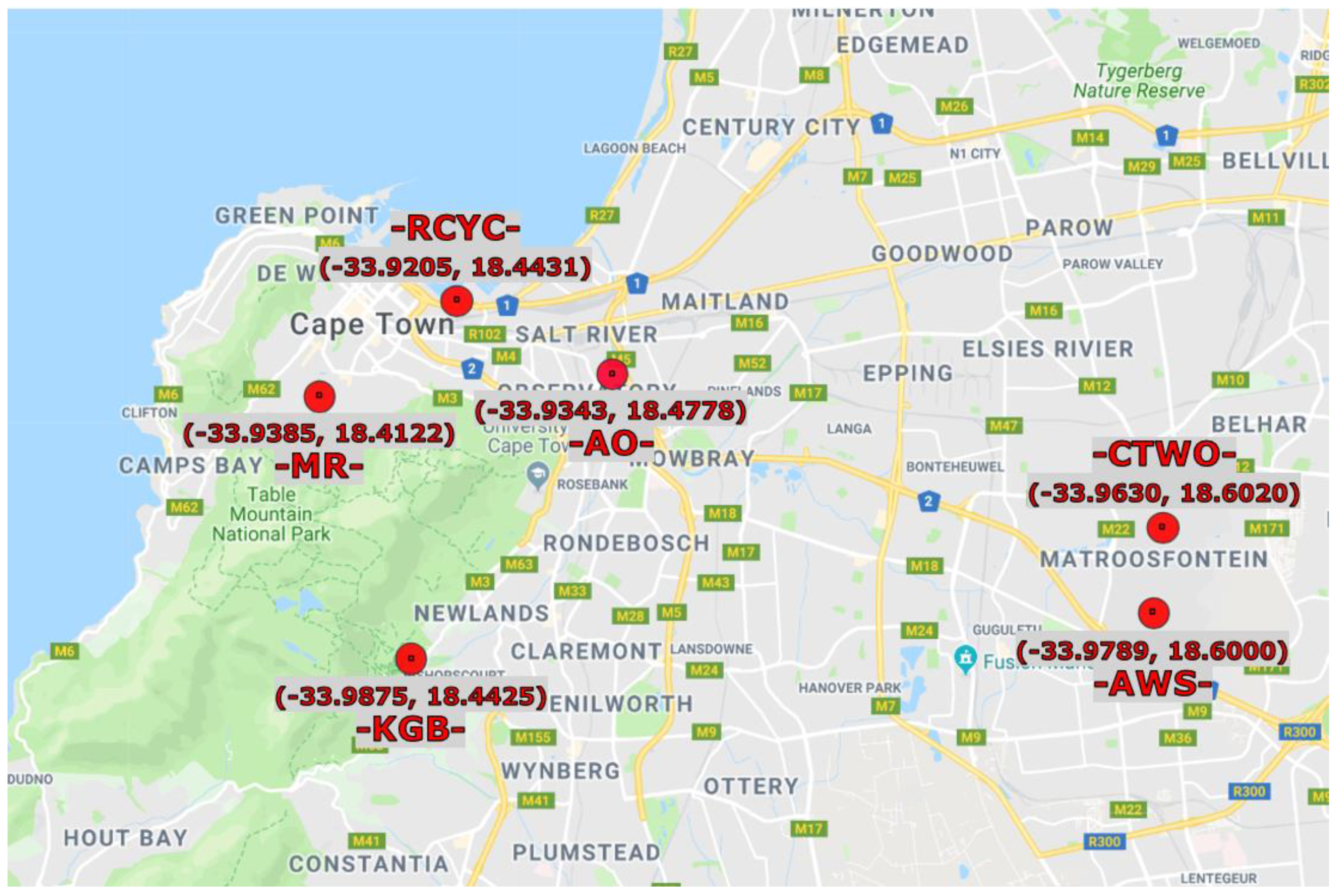
2.1. Measurement Locations and Data

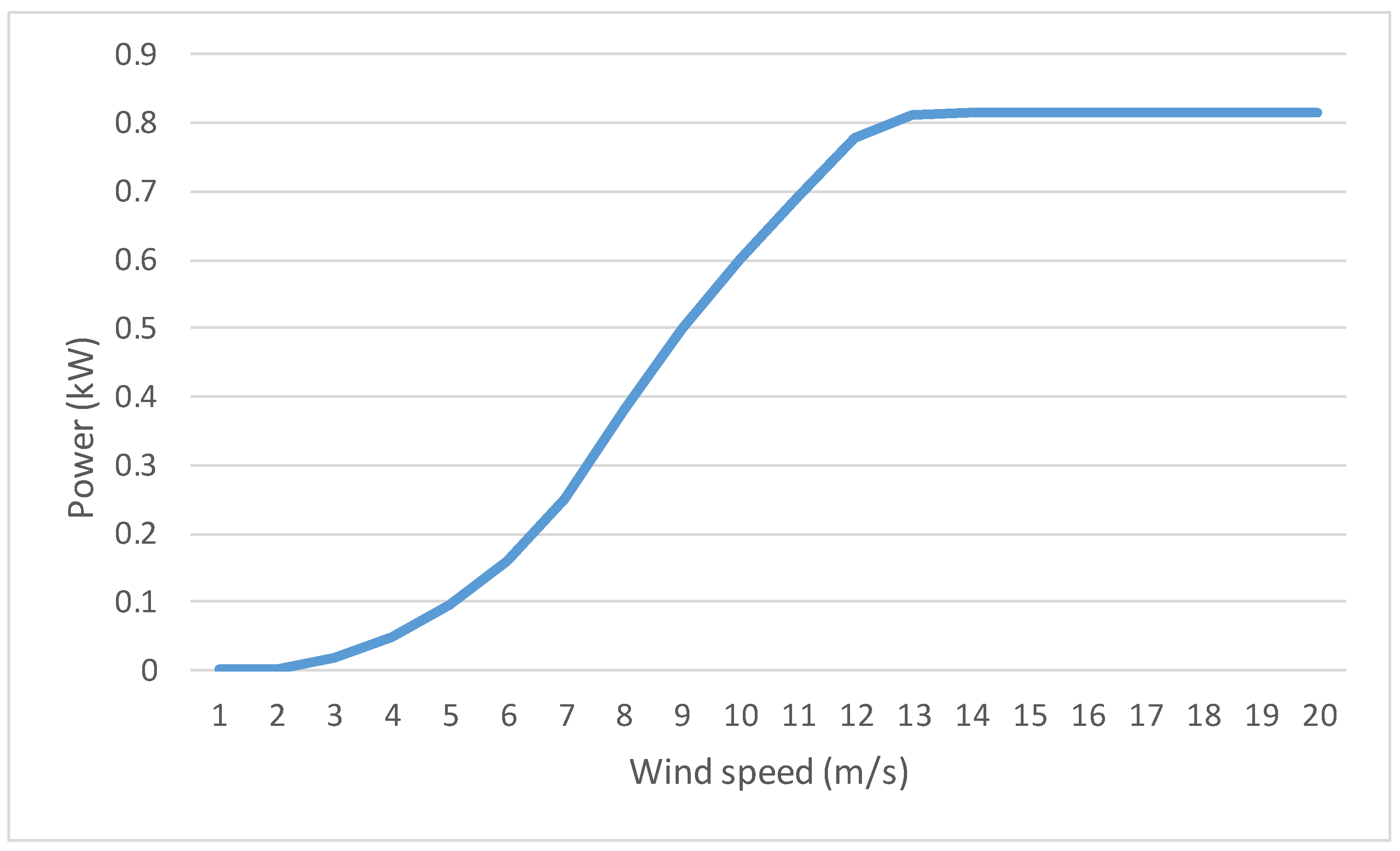
Six sites were chosen with existing weather measurement stations, installed and maintained by the South African Weather Service (SAWS), which provided the data used in this study. Wind recordings made at five-minute intervals from 1 January 2015 to 31 December 2016, corresponding to 731 days (210,600 recordings per site), were provided by SAWS. All stations used RM Young (R. M. Young Company, MI, USA) wind sensors.

In addition to the weather data being publicly accessible, the six sites span the Cape Town metropolitan area, representing different regions and topologies. With this being the first study to perform such urban wind resource mapping for Cape Town, it was decided to use these six sites as a starting point due to data reliability and public accessibility, in addition to traversal of the metropolitan area. Should urban wind power deployment in Cape Town become of interest, future studies can build on these results using more test sites and/or measurements. Details about the weather stations were provided to the authors directly by Mr. M. Mkhwanazi of the SAWS by means of an email communication on the 25 May 2017. The locations of the six stations are visualized in Figure 1 and the details for every station are listed in Table 1. The figure shows that the six stations traverse the Cape Town metropolitan area with its different topologies. The following paragraphs provide details of each of the six stations.

The first measuring station is named the Royal Cape Yacht Club (RCYC), inside the Table Bay Harbor at a height of 11 m above sea level. This site was chosen for this study due to its position on the coastline with strong on- and off-shore breezes. The site has been used by SAWS since 2001 but the particular weather station used to provide the data for this study has been in operation since 2011.

The second station is called the South African Astronomical Observatory (SAAO). It is located in Observatory, Cape Town, at a height of 15 m above sea level. The station has been used for weather recording since 1841 and the most recent upgrade was in 2009. The surrounding area is characterized by open fields with a mix of low-rise residential and commercial buildings. The AWS, along with the third and fifth stations, passed the most recent SAWS verification, maintenance, and conformance report in February 2017, conforming to standards laid out by the World Meteorological Organization (WMO) Commission for Instrument and Methods of Observations Guide (CIMO) [26].

The third station, Kirstenbosch Botanical Gardens (KBG), is located in Kirstenbosch at an altitude of 156 m above sea level and has been in use since 1999. The current setup of the weather station was installed in 2010. This location was chosen as it is one of the few recording stations on the southern side of Table Mountain with numerous residential suburbs in surrounding areas and should, therefore, give a good indication of the resource potential for residential-scale wind turbines therein.

The fourth station is the Molteno Reservoir (MR) station, located in the Oranjezicht suburb at an altitude of 98 m above sea level. This site was chosen because of its location in a residential suburb on the northern slope of Table Mountain, providing data on the urban wind regime in Oranjezicht.

The fifth station was the Cape Town Automatic Weather Station (AWS) located near Cape Town International Airport at an altitude of 46 m above sea level. This station was chosen as one of two (along with the sixth) sites located in the vicinity of the International Airport. The area is characterized by open fields and runways with a small number of commercial buildings.

The sixth and final dataset used in this study was obtained from the Cape Town Weather Office (WO) station also located at the International Airport, albeit 1.92 km away from AWS. A comparison may highlight wind regime variation over short to medium distances within the same topology.

The recording heights at each station varied. To have a consistent and comparable set of wind speed measurements, the recordings at each location were adjusted using the Prandtl logarithmic law equation [27]:

$$V_z=\frac{U_{\ast }}{k}\ln \left(\frac{z}{z_0}\right)$$

(3)

with $V_z$ being the wind speed at the chosen height, U_* the recorded wind speed, k the von Karman constant (taken as 0.4), $z$ the height above ground, and $z_0$ the roughness length. For this study, the roughness length was taken as being equal to 1 [28]. This roughness length was chosen as the locations used in this study can be classified as a mix between “suburban” and “urban” according to the classification in Reference [27]; or as “closed” according to Reference [28]. In the latter classification, “closed” is defined as: “Landscape totally and quite regularly covered with similar-size large obstacles, with open spaces comparable to the obstacle heights; e.g., mature regular forests, homogeneous cities or villages” [28]. After revisiting the topology of the sites, it was concluded that this classification best suited the six locations. None of the locations are sited in the city center of Cape Town, in which case using a roughness length of larger than 1 would be required, as described in [23]. These adjusted wind speeds were then used for the remainder of the study.

Determining the exact roughness length at an urban location is extremely challenging, as shown by the significant amount of literature available on the subject and the derivation thereof is outside the scope of this paper. In this study, a roughness length was determined for the sites in accordance with their topology and environment, which is in line with other studies [28,29]. Each of the locations can be described by a roughness length of 1, as they are surrounded by common residential or one-story buildings. [29] There are challenges associated with the use of Equation (3) within the urban wind environment. These challenges have led to the development of modified equations for extrapolating wind speeds from different heights in the urban environment [29,30].

The western cape region of South Africa experiences lower wind speeds in winter when compared to the summer months and this can be attributed to structure and strength of the upper tropospheric jet stream. The stronger summer winds (most pronounced in December) are due to the South Atlantic high-pressure cell. In the Cape Town region, a daily peak of wind speeds generally occurs between 16:00 and 20:00 when the sea breeze circulation works in addition to the southerly gradient winds and summer minimum wind speeds occur around 06:00 and in winter this minimum wind speed occurs at approximately 10:00 [31]. The strong southeast breeze that is a common occurrence in Cape Town occurs for approximately 70% of the time during the summer period (November to March) while the South-Easter is only present for 40% of the time in June [32].

2.2. SWT Models

Following a review of similar previously published small-scale urban wind power studies, four widely-used SWTs were identified: (1) SkyStream 3.7 manufactured by Xzeres; (2) Kestrel e230i manufactured by Kestrel; (3) eddyGT manufactured by Urban Green Energy; and (4) the Turby turbine manufactured by Core International with research assistance from the Delft University of Technology. The detailed specifications of the SWTs are shown in

Table 2. Wind turbine specifications.

Turbine Name	Kestrel e230i	SkyStream 3.7	eddyGT	Turby
Turbine type	HAWT	HAWT	VAWT	VAWT
Rated output (W)	800	2 400	1000	2 500
Rated wind speed (m/s)	12.5	13	12	14
Cut in wind speed (m/s)	2.5	3.5	3	4
Rotor diameter (m)	2.3	3.72	1.8	2
Number of blades	3	3	3	3
Swept area (m2)	4.2	10.9	4.62	5.3

[12,33].

The first two (the SkyStream and the Kestrel) are Horizontal Axis Wind Turbines (HAWTs) while the other two are Vertical Axis Wind Turbines (VAWTs). Two HAWTs and two VAWTs were chosen to assess which of the two turbine types was best suited to the specific wind regime at the chosen locations. The SkyStream and the Turby are larger and have a higher-rated output compared to the Kestrel and the eddyGT, respectively. This comparison was done to assess whether a small-scale turbine with a higher-rated capacity is better suited to the urban environment compared with a very small-scale turbine. All four selected SWTs have been well studied and have a proven track record in small-scale applications and thus can together reflect and represent the current state of SWT technological specifications.

The power curves for the four turbines were obtained from the Wind Power Program Wind Turbine Database [34]. As these power curves have been derived from the manufacturers’ data, it would be prudent to presume that these power curves overestimate real-world performance, since real-world power output of a turbine is dependent on numerous factors that may not be fully accounted for in a laboratory setting normally used by manufacturers to calculate power curves. Thus, the produced energy given by these wind turbines is seen as an upper limit to what can be expected if a wind turbine is installed in the field. Research concerning the differences between the expected energy generated using the manufactures power curve and the in-situ experiences of wind turbine operators has led to the development, in some instances, of a scaling law [35]. However, where this scaling law is applicable, it is highly susceptible to the local wind conditions and therefore the authors of [35] recommended that a recalibration of the turbine’s power curve is done post-installation.

As there were no wind turbines installed at the locations in this study, the manufacturer’s power curves were used without any changes being made to the curves. Wind turbine manufacturers are required to provide power curves based on the IEC 61400-12-1 standard [5] and the use of this standard should help to minimize any significant variation between the manufacturer’s power curves and the in-situ measurements.

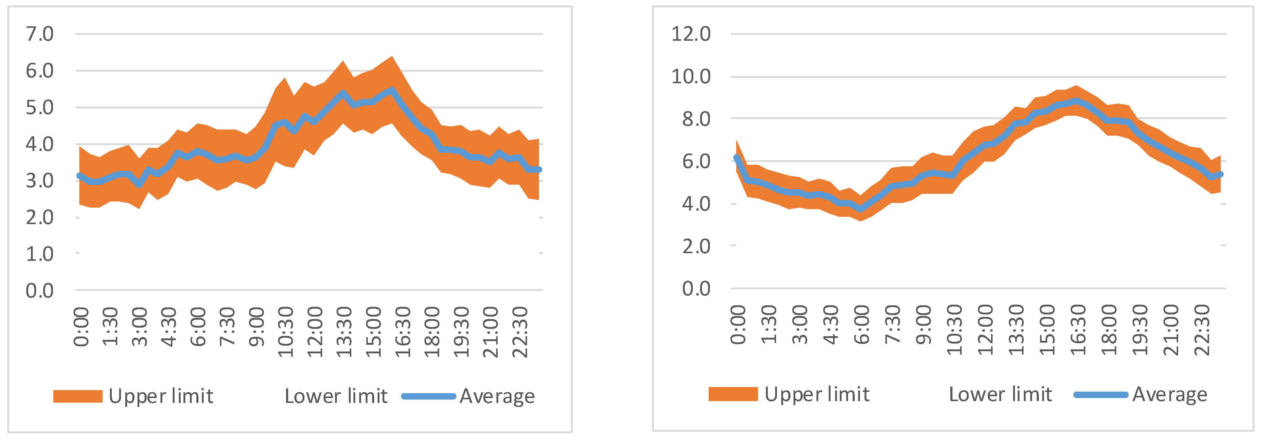
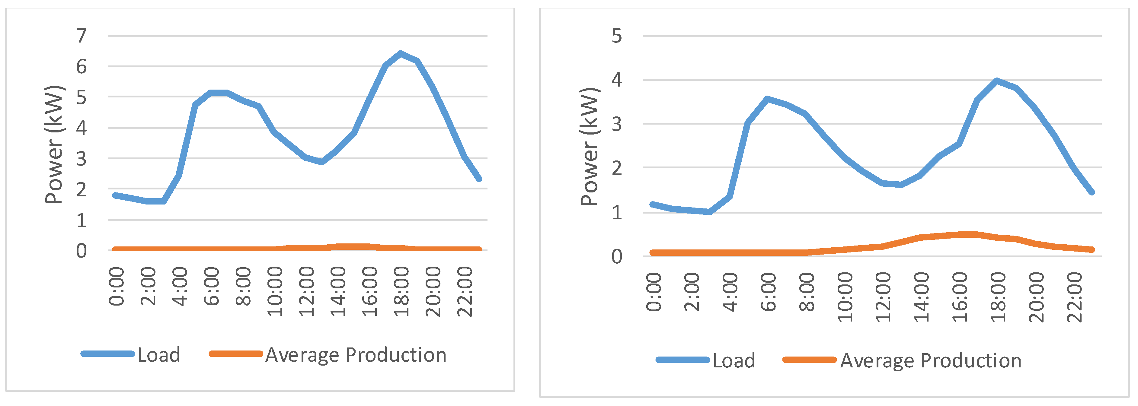
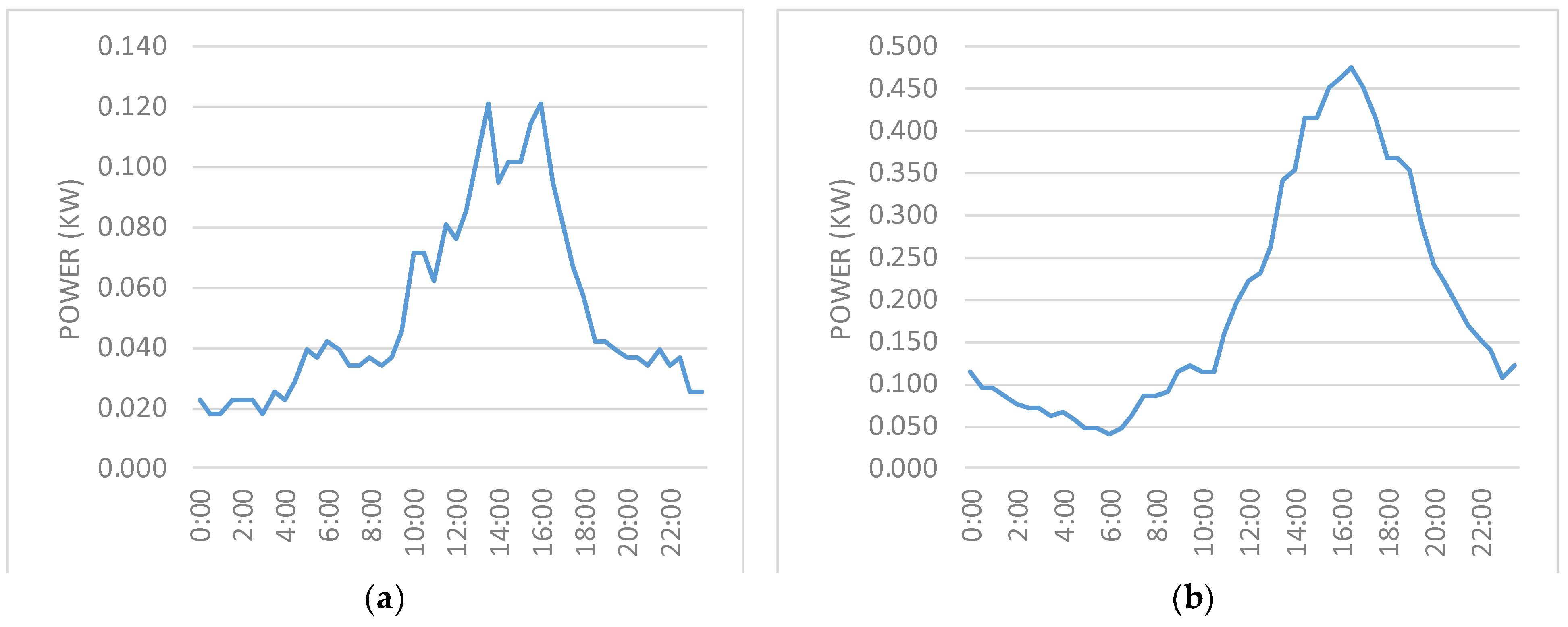
2.3. Expected Diurnal Electricity Generation

The daily electricity generation profiles for two different days at a chosen location were analyzed. This was done to investigate at what period of the day a small-scale turbine would be producing electricity. It is beneficial to investigate these generation curves as they show to what extent the amount of electricity generated from a small-scale wind turbine matches the typical demand profile at any period of time during the day.

An analysis of the daily power output of the wind turbine at the same location was carried out over two different months. This was done for two reasons. Firstly, it was done to identify the average daily power output profile of the wind turbine for the months and to investigate the variability associated with the urban wind regime over a period of time. Secondly, the analysis was done to investigate the variability of the wind regime over a month.

The Cape Town WO site was chosen for this section of the analysis, and the Kestrel e230i turbine power curve was chosen as the representative small-scale power turbine. The five-minute wind speed data for the site for two different days (21 June 2016 and 21 December 2016) were used to calculate the expected electricity generation of the turbine at each location.

These two days were chosen as they represent peak winter and summer in the southern hemisphere. The days that were chosen (and the months June and December, as well) were chosen to be a representative of typical winter and summer days (months).

June and December were chosen to investigate the average hourly generation patterns over the two months. The power curve from the Kestrel e230i turbine was then applied to the average five-minute wind speeds from the site and the estimated amount of electricity generated was recorded. The electricity produced per five-minute interval by the turbine was then compared against typical residential load profiles for winter and summer, respectively.

2.4. Cost of Electricity

The Levelized Cost of Electricity (LCOE) metric is a well-known and often-used method of evaluating the costs of generating electricity from different technologies [36].

The LCOE metric returns the cost of generating electricity over the lifetime of the turbine per kilowatt hour (kWh) and for this study it included the capital costs of the Kestrel e230i turbine, the installation costs (including transport and site preparation costs, and the maintenance costs associated with operating the turbine over its 20-year lifetime). These costs were obtained directly from the manufacturer of the Kestrel turbine by the authors. These costs were then discounted back to present value using a discount rate of 8.4%. This is the rate used by the South African Department of Energy during the process of developing the 2016 version of the Integrated Resource Plan for electricity [37]. This discount rate was used as it provides a well-grounded reference point for energy investments in South Africa. Other investors may have significantly different discount rates and, as such, a sensitivity analysis was conducted on the discount rate using the AEP values of the WO site.

The costs were converted from South African ZAR to Euros by the average exchange rate during the month of September 2017 which was 1 EUR = 15.68 ZAR [38]. The discounted costs were then summed over the 20-year lifetime of the turbine and divided by the total amount of electricity that the turbine is expected to produce over its lifetime.

The LCOE formula is given by the following equation [36]:

$$LCOE=\frac{{{\displaystyle \sum }}_{t=0}^n\frac{I_t+M_t+F_t}{{\left(1+r\right)}^t}}{{{\displaystyle \sum }}_{t=0}^n\frac{E_t}{{\left(1+r\right)}^t}}$$

(4)

with $I_t$ being the investment expenditure in year t, $M_t$ the maintenance costs in year t, $F_t$ the fuel costs in year t (for this study there are no fuel costs), r the discount rate, $E_t$ the electricity generated in year t, and n the total life of the wind turbine.

The Kestrel e230i turbine was selected for this LCOE analysis because it is made in South Africa and reliable cost data for it could be accurately sourced. The other three turbines are not manufactured in South Africa and thus accurate cost data could not be sourced. In addition, the costs associated with importing the turbine may inflate the overall project cost.

3. Results

The average recorded wind speeds varied significantly from station to station. The station with the highest average wind speed for the whole two-year recording period was the WO station with a wind speed of 5.05 m/s. The lowest average wind speed was 2.04 m/s, recorded at the Kirstenbosch recording station. The average of all six stations for the two-year period was 3.24 m/s. The data were averaged from the two years to take into account any inter-annual fluctuations in the wind speeds. Of the six recording stations, five o experienced seasonal fluctuations in their average monthly wind speeds with only the Kirstenbosch station showing no signs of higher wind speeds in the summer period. The seasonal fluctuations, as well as the monthly average wind speeds for all six stations, are shown in Figure 2. The figure shows that the WO station consistently has the highest average monthly wind speeds and the Kirstenbosch station has the lowest recorded average wind speeds for the majority of the year.

With the recorded wind speed at intervals of five minutes being the input of this analysis, the output would be to obtain the expected generation capacity and LCOE for an SWT installed at each location. The detailed step-by-step analysis procedure to obtain those results is demonstrated in Section 3.1 on the WO Station since it is the one with the highest average wind speed across the year. In Section 3.2, the final results for all stations and SWT models are presented.

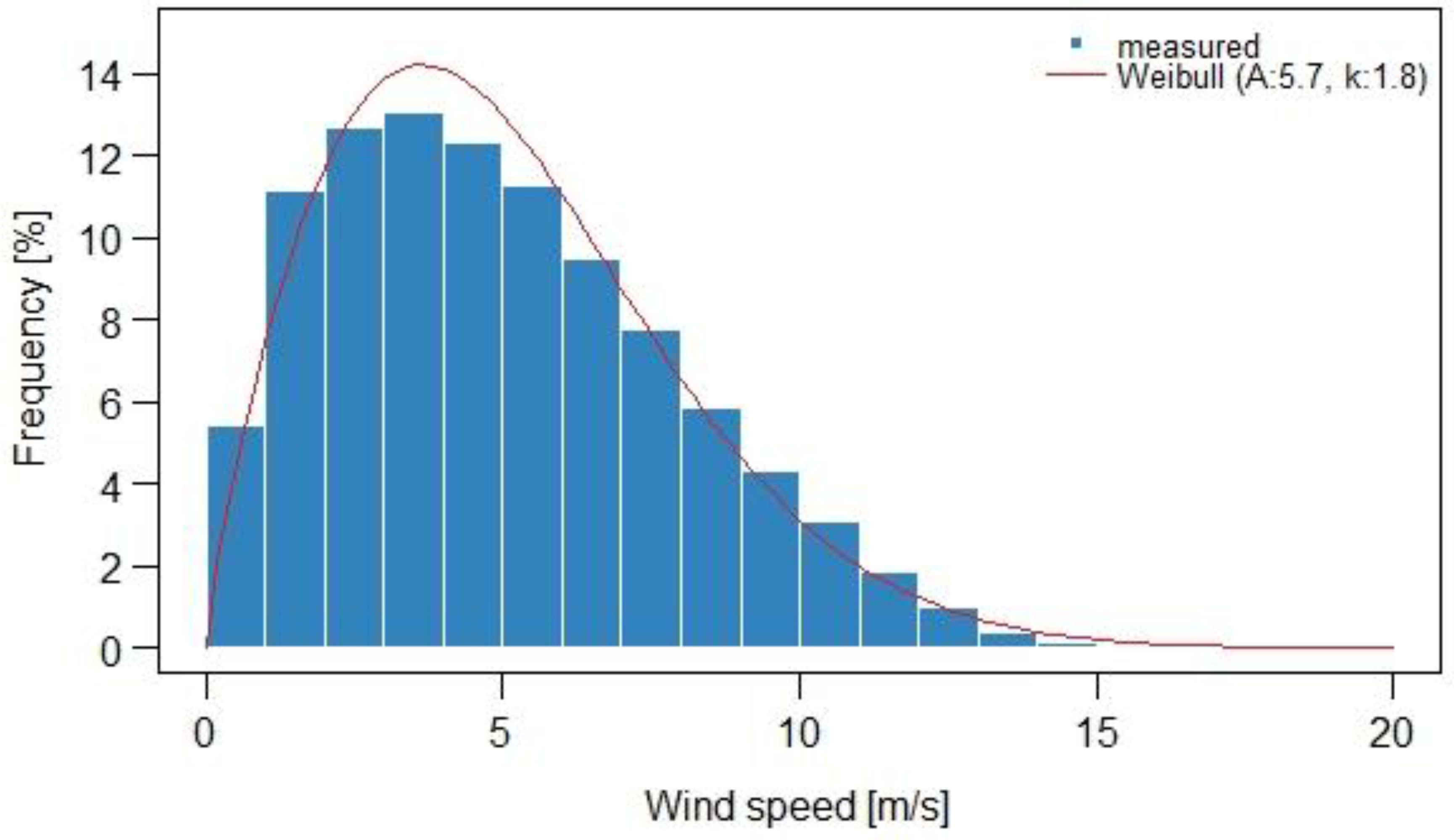
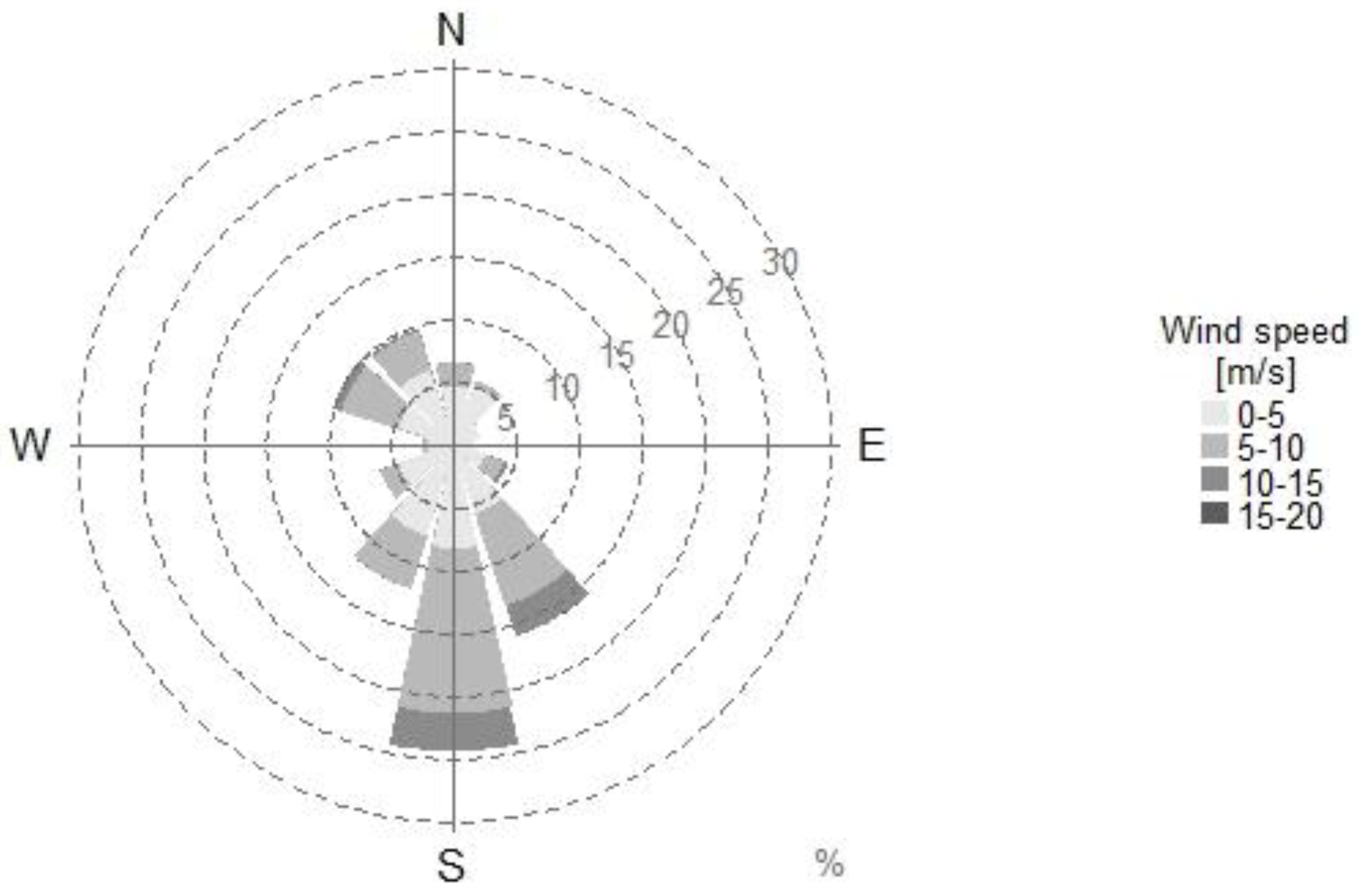
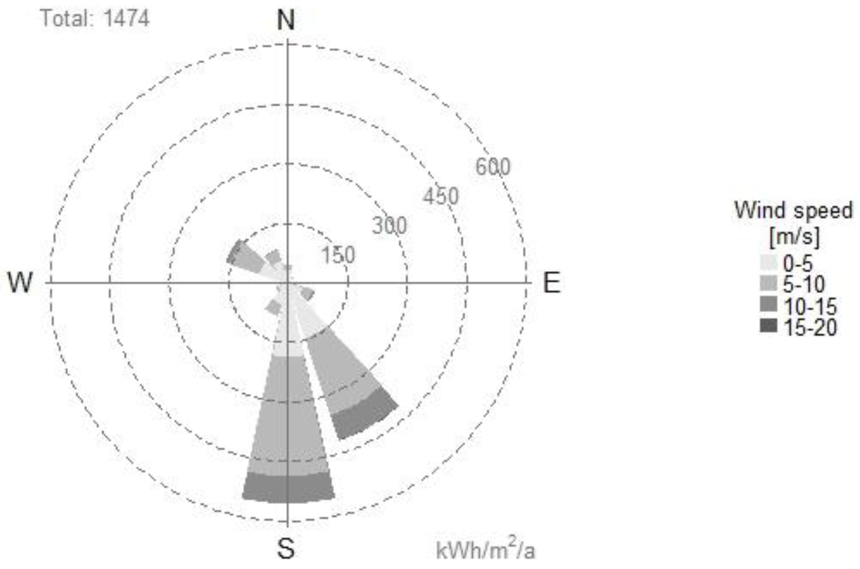
3.1. Analysis Procedure: Demonstration using WO Station

The wind rose for the Cape Town WO station is shown in Figure 3, illustrating that the majority of wind speeds recorded at this station are within 5–10 m/s and the prevailing wind direction is from the South. The wind speed varied significantly at all measuring stations and this variability was pronounced even at similar times throughout consecutive days. Figure 4 shows comparison of the wind speeds experienced at the WO station for the months of June and December 2016. The figure shows the average wind speed as well as a 95% confidence interval of variation in the average wind speed. It can be seen that the wind speeds are, in general, lower and more varied in June.

The next step in the analysis of the wind data was to calculate the Weibull parameters. A shape parameter (k) of 1.8 and a scale parameter (c) of 5.7 m/s were determined. These values were then used to plot the Weibull probability density function, as illustrated by the red line in Figure 5. The blue columns (histogram) in Figure 5 represent the wind speed distribution of the recorded data. The Weibull curve has a coefficient of determination of 0.97, which indicates that the Weibull curve is an accurate fit of the recorded data. Further evidence of the good fit between the recorded data at the WO station and the station’s predicted Weibull curve is the station’s RMSE value, which was calculated at 0.0088 Hz.

Using the developed Weibull, the theoretical wind energy resource potential was estimated for the WO site. This is shown in Figure 6. The total (annual) energy available at the site was calculated [5] to be 1474 kWh/m²/year. This calculation was done based on the standard IEC cubic power law for obtaining the amount of energy in a wind stream [5]. Once again, Figure 6 demonstrates that the majority of the wind energy comes from wind speeds of 5–10 m/s and from the south (dominant wind direction).

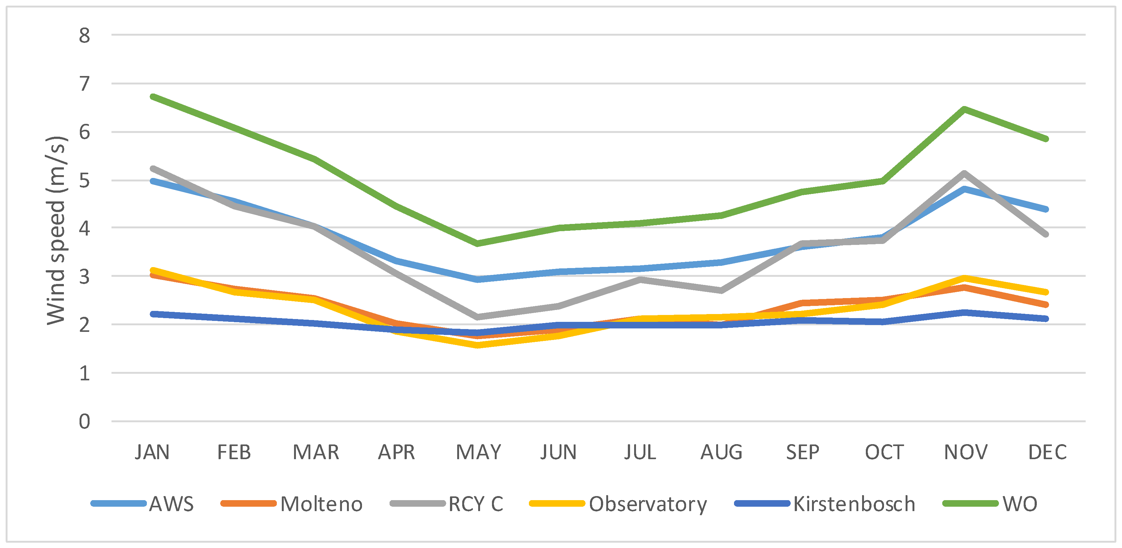
3.2. Results for All Stations

Following the step-by-step demonstration of the analysis procedure at the WO station, the methodology was applied for all six stations spanning Cape Town. The full results (average wind speed, energy resource potential, AEP and capacity factor for each turbine type) at each of the six stations are shown in

Table 3. Summary of results for the six stations.

Station	RCYC	Kirstenbosch	AWS	Molteno	Observatory	WO
Average wind speed (m/s)	3.61	2.04	3.83	2.35	2.33	5.06
Energy resource potential (kWh/m²/year)	1181	80	610	189	145	1474
Kestrel AEP (kWh/year)	1224	19	982	259	199	1636
Kestrel Capacity Factor	0.172	0.003	0.14	0.036	0.028	0.229
SkyStream AEP (kWh/year)	3301	13.73	2401	518	339	4304
SkyStream Capacity Factor	0.155	0.001	0.11	0.024	0.016	0.203
eddyGT AEP (kWh/year)	784	4.33	523	119	85	975
eddyGT Capacity Factor	0.138	0.001	0.09	0.021	0.015	0.171
Turby AEP (kWh/year)	2406	0.659	1227	195	85	2730
Turby Capacity Factor	0.11	0	0.06	0.009	0.004	0.12

. The AEP values were obtained by using both the wind speed distribution at each location and the respective wind turbine power curve.

Using the wind speed data from each of the stations, the theoretical wind energy resource potential was calculated, as shown in Figure 7 and Table 3. It is clear to see that the annual energy resource potential varies between the stations included in the study. It is evident that the WO station has the highest energy potential with a value of 1474 kWh/m²/year, while the Kirstenbosch station has the lowest energy potential with a value of 80 kWh/m²/year. These results are expected as these two stations also have the highest and lowest average wind speeds, respectively.

Comparing the Kirstenbosch station to the WO station, the Kirstenbosch station only has approximately 5% of the wind energy potential of the WO station. This again highlights the variability of the wind resource depending on the location.

3.2.1. Comparison of Wind Turbines

Following the assessment of the wind resource potential at the locations studied, the power curves for the four small-scale wind turbines were applied to the wind energy resource potential of each site to simulate the energy output of a turbine installed at these locations. As highlighted above, the raw wind speeds for all of the locations were corrected to a constant hub height of 20 m. This was done so that the results of the calculations are comparable.

The power curve of the kestrel turbine is shown in Figure 8. The turbine has a cut-in wind speed of 2.5 m/s and approximately proportional relationship with wind speed and thus there is more available power at wind speeds of 5–10 m/s even if the most frequent wind speeds are within 4–6m/s.

The overall results for all six stations and all four of the chosen turbines are summarized in Table 3. The table shows a significant variation in nearly all of the parameters calculated. Across the six locations, the Kestrel turbine produced an average of 681.89 kWh/year with an average capacity factor of 10.1%, the SkyStream produced an average of 1813.29 kWh/year with a capacity factor of 8.53%, the eddyGT produced 415.63 kWh/year and its capacity factor was 7.3%, and finally the Turby produced 1107.63 kWh/year with a capacity factor of 5.06%.

The HAWTs performed better than their VAWT counterparts at every location despite the HAWTs having a smaller-rated capacity (the Kestrel has a rated capacity of 800 W vs. the eddyGT’s capacity of 1000 W and the SkyStream has a capacity of 2400 W vs. the Turby’s 2500 W).

The key to the HAWTs having better performance could be attributed to their lower cut-in wind speed relative to the VAWTs. This allows the HAWTs to take better advantage of the low average wind speeds generally experienced in urban areas.

3.2.2. Expected Diurnal Electricity Generation

This subsection provides information on the electricity production of a small-scale turbine with an interval of five minutes at the WO station on two different days. These generation curves are then compared against typical daily demand profiles to identify if there are periods of the day when the generation curve follows the same shape as the demand profile.

The power curve from the Kestrel e230i is shown in Figure 8. The Kestrel turbine was selected because it is the turbine with the average highest capacity factor out of the four small-scale wind turbines chosen for this study as it is readily available in South Africa.

The Cape Town WO station was chosen as it is the site with the highest wind energy resource potential of all of the six locations. For the WO site, two days were selected, one representing the summer wind regime and the other representing the winter wind regime: 21 December 2016 was chosen to be representative of the summer wind conditions as it is the summer solstice in the southern hemisphere, while 21 June 2016 was selected as being representative of the winter wind conditions as it is the winter solstice in the southern hemisphere.

Figure 9 shows a comparison of the expected energy production vs. the typical demand of a South African household during winter and summer. The average wind speeds for summer and winter were derived from the average wind speeds during three months (December, January, and February for summer, and June, July, and August for winter) The results show that the expected electricity production from the wind turbine during winter is negligible. There is a small contribution from the wind turbine towards the residential load in the summer months but, again, it is a very small contribution, as shown in Figure 10.

The results from the seasonal generation curves from the two sites once again show the seasonal fluctuations that were evident in the monthly wind speeds of the various locations.

Looking at the average hourly wind speeds and energy production for the months of December and June 2016 yield similar results. The average daily electricity production for the Kestrel turbine at the WO station for December and June 2016 were calculated to be 4.68 kWh and 1.24 kWh per day, respectively.

The average power generated by the Kestrel turbine for the months of June and December 2016 at the WO station is shown in Figure 10. Figure 10 (left) shows that there is, on average throughout the month of June, a slight rise in the power generated by the turbine in the early afternoon, which decreases at around 18:00. The maximum power generated by the turbine for this month is approximately 120 W. Figure 10 (right) shows a similar result but with a slightly lower variation in the maximum power generated by the turbine between 21 December and the average values for that month. The maximum power generated on 21 December was approximately 700 W while on average the maximum power generated by the turbine for the month of December was 476 W. The limited production of the turbine in June can be attributed to the generally low wind speeds experienced during that time with short gusts of wind producing a nominal amount of electricity.

3.2.3. Cost of Electricity

Table 4. Levelized Cost of Electricity (LCOE) values for the six locations.

Station	LCOE (Eur/kWh)
Royal Cape Yacht Club	0.35
Kirstenbosch	22.59
Automatic Weather Station	0.44
Molteno reservoir	1.66
Observatory	2.15
Cape Town Weather Office	0.26

shows the results of the Levelized Cost of Electricity (LCOE) analysis that was carried out using the Kestrel e230i as the reference wind turbine. As shown in table, there are no locations where the LCOE value is below the residential tariff for users of more than 600 kWh in the City of Cape Town, which stands at approximately €0.15/kWh.

A sensitivity analysis was done on the discount rate used in the LCOE formula. Discount rates ranging from 8% to 18% were studied and, as the discount rate increase, the LCOE value also increased, which meant that, for the discount rates studied, the LCOE values are always above the current residential tariff for electricity in the City of Cape Town for users of more than 600 kWh per month (approximately €0.15/kWh).

The significantly large LCOE value for the Kirstenbosch station is due to the very limited electricity production experienced at that station. As shown in

Table 5. Estimated amount of electricity generated at each station.

Station	Electricity Generated (kWh/year)
Royal Cape Yacht Club	1225
Kirstenbosch	19
Automatic Weather Station	982
Molteno reservoir	259
Observatory	200
Weather Office	1637

, the production at the Kirstenbosch site is two orders of magnitude smaller than the best performing station, the WO station.

4. Discussion

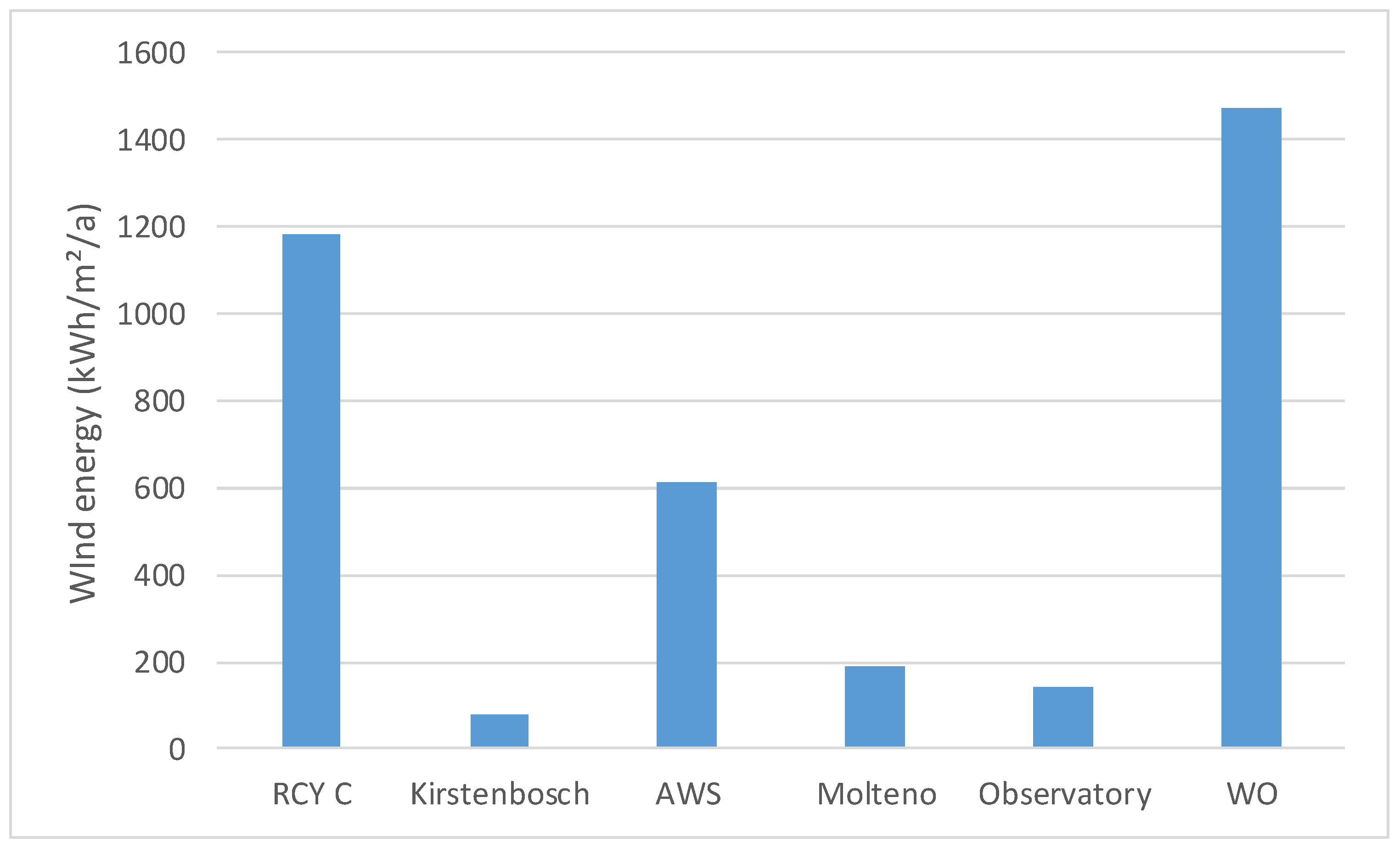
4.1. Quantification of the Urban Wind Potential in Cape Town

According to the conducted literature review at the time of this work, this is the first study that examined, in detail, the urban wind resource potential of several locations in Cape Town.

Out of the six chosen locations, three of the locations (Royal Cape Yacht Club, the Automatic Weather Station (AWS), and the Cape Town Weather Office (WO)) initially showed potential for the installation of a small-scale wind turbine, with the HAWTs having higher AEP values at each of the six locations compared to their VAWT counterparts.

The results of the wind resource assessment are summarized in Table 5. These three locations were situated in non-residential areas. The three locations that were situated in residential areas had much lower wind resource potential. This may be due to the increased number of obstructions (houses and trees) in residential areas when compared to the non-residential locations that were selected for this study.

The findings of this study are consistent with other studies on wind speed assessments of Cape Town [31,32]. The seasonal and daily fluctuations are in line with previous studies. Field measurements, as opposed to computational simulations (e.g., CFD), were used, with this being the first attempt to quantify the potential for urban wind energy in Cape Town. The results show that the potential for urban wind energy at the six locations is limited and not cost-effective and thus it may be difficult to justify conducting detailed CFD simulations.

Cape Town, and South Africa in a wider context, is experiencing rapid urbanization coupled with electricity shortages. Therefore, the impact of urbanization on the wind regime in Cape Town will increase, which will make reliable and accurate urban wind energy resource assessments more complex even if the desire to install small-scale wind turbines increases.

4.2. Comparison of the Different Wind Turbine Types

The two Horizontal Axis Wind Turbines (HAWTs) used in this study had higher Annual Energy Production (AEP) values than their Vertical Axis Wind Turbine (VAWT) counterparts in both electricity produced and capacity factors. These findings are expected and are consistent with previous research in this area [33]. This is shown in Table 3. The Kestrel e230i and the eddyGT AEP values are comparable as they are the two smaller turbines with similarly-rated outputs. Likewise, the SkyStream 3.7 and the Turby are comparable as they are the two larger turbines. The difference in the AEP values is possibly due to the lower cut-in wind speeds of the HAWTs compared to the cut-in wind speeds for the VAWTs. These cut-in wind speeds are shown in Table 2, which also highlights the specifications of the various turbines. VAWTs and HAWTs use different forces to generate electricity. HAWTs rely on drag force while the Savonium type VAWT uses drag force and the Darrieus VAWT uses lift force as well. Both VAWTs used in this study were of the Darriues type and this might explain some of the difference in production values for the different turbines. [39].

This finding does not conclusively show that HAWTs are better suited to extracting energy from the urban wind regime in all situations but there is a clear trend to be seen from the results of this study. A low cut-in wind speed allows a turbine to start generating electricity at lower wind speeds and the urban wind regime is characterized by low wind speeds. This study used a wind turbine’s annual energy production (AEP) as the sole criterion when judging the turbine’s performance.

4.3. Daily Electricity Generation

The daily generation profile curves were generated for the WO location over two separate days. This was done to evaluate at what times during the day a typical turbine is expected to generate electricity. The results from the Cape Town Weather office combined with the power curve of the Kestrel e230i turbine show that, on 21 June, there is negligible energy production at the site and only a limited production of electricity on 21 December. The Cape Town WO station generated 4.4 kWh, where the typical demand for electricity per household may be in the region of 20 kWh per day, assuming a monthly electricity usage of 600 kWh. Therefore, it is not recommended to install SWTs at this location. This section of the analysis further highlighted the variability of the wind resource potential not only between the two sites but also showed the seasonal and inter-day fluctuations of electricity generation.

4.4. Cost-Effectiveness of a Small-Scale Wind Turbine in Cape Town

The results from the Levelized Cost of Electricity (LCOE) analysis (detailed in Table 5) using the Kestrel e230i wind turbine show that electricity generated from small-scale wind turbines in Cape Town is not currently cost competitive. The lowest LCOE value for the Kestrel turbine with a hub height of 20 m was €0.26/kWh, which is higher than the current domestic electricity tariff in Cape Town for households who use more than 600 kWh per month which stands at €0.15/kWh (refer to Section 2.4). The LCOE analysis was also done for the Kestrel turbine but at a height of 30 m above the ground, which resulted in a decrease of the LCOE value at the WO station to €0.22/kWh. This is because the turbine will generate more electricity at a greater height. Even at this greater height of 30 m, the LCOE of electricity generated from the turbine is still €0.07 more than the cost of using electricity provided by the City of Cape Town. However, it is expected that the cost of obtaining electricity from the City of Cape Town will continue to increase in the coming years. That in addition to the technological advancement of SWT and the expected decrease in their costs, they are likely to become more cost competitive in the future.

The results of the discount rate sensitivity analysis show that, even at high discount rates (18%), the electricity produced by the Kestrel wind turbine at the best performing location is more expensive than the current domestic tariff for residential users over 600 kWh per month in the City of Cape Town.

4.5. Viability Small-Scale Wind Turbine in Cape Town

The results of the study show that there is technical potential for small-scale urban wind turbines at certain locations in Cape Town. However, the significant variability associated with the resource indicates the need for detailed wind speed recordings at each potential site.

Even then, the wind resource at the location may not be sufficient to warrant the installation of a small-scale turbine. The results of the urban wind resource mapping coupled with the LCOE analysis establishes that, currently, the use of small-scale wind turbines to generate electricity in Cape Town is neither viable nor cost-effective.

It should be noted that the results presented in this paper have not been validated by real-world experiments. There are a number of reasons why the energy production values of an SWT may vary from the theoretical calculations [33]. Due to these factors, which include fluctuations in the wind resource, turbine degradation, and changes in the surrounding urban environment, the actual electricity produced may vary significantly from the results presented in this study and, thus, these results should be seen as an upper limit of typical electricity production for an SWT at these six locations. In projects where verification of the calculated energy production has been carried out, the actual energy production was below the predicted [14,15]. While the exact amount of overestimation of energy production varies from project to project, the authors of [14] set out some guidelines to help reduce the discrepancy between the predicted and actual energy production values.

5. Conclusions

The urban wind energy potential of Cape Town was quantified in this study by analyzing high-resolution, annual wind speed measurements taken from six locations spanning the city. The two-parameter Weibull distribution was used to derive the PDF and CDF for wind speed at each location. These data were then used to determine the AEP corresponding to four different SWT models (Kestrel e230i, SkyStream 3.7, eddyGT, and Turby) at each of the locations. The main challenge faced in this study was the estimation of the wind speeds at heights different to those at which they were measured. This is due to the complex nature of the urban wind environment. Future studies should endeavor to make sure that the wind data used are as representative as possible.

The results show that the two HAWTs had higher AEP values in all six locations compared to their VAWT counterparts, in terms of both electricity produced and capacity factors. This may be due to the lower cut-in wind speeds of the HAWTs. The three more densely populated areas (WO, AWS, and RCYC) had higher AEP values than the less-populated ones (Molteno reservoir, Observatory, and Kirstenbosch). The analysis showed that the urban wind energy regime is characterized by significant variability across distance as well as time. Seasonal fluctuations in wind speed were also pronounced for five out of six stations. Calculation of LCOE showed that electricity generated by SWTs is currently more expensive than buying electricity from the existing grid infrastructure. This may change in the future as the price of grid electricity in the South Africa market is expected to increase, and also as a result of advancements in SWT technology.

References

1. Syngellakis, K.; Carroll, S.; Robinson, P. Small Wind Power: Introduction to Urban Small Scale Wind in the UK. Refocus 2006, 7, 40–45. [Google Scholar] [CrossRef]
2. Palma, J.M.L.M.; Castro, F.A.; Ribeiro, L.F.; Rodrigues, A.H.; Pinto, A.P. Linear and Nonlinear Models in Wind Resource Assessment and Wind Turbine Micro-Siting in Complex Terrain. J. Wind Eng. Ind. Aerodyn. 2008, 96, 2308–2326. [Google Scholar] [CrossRef]
3. Lotfi, M. Atmospheric Wind Flow Distortion Effects of Meteorological Masts. Master’s Thesis, FEUP, Porto, Portugal, 2015. [Google Scholar]
4. Walker, S.L. Building Mounted Wind Turbines and Their Suitability for the Urban Scale—A Review of Methods of Estimating Urban Wind Resource. Energy Build. 2011, 43, 1852–1862. [Google Scholar] [CrossRef]
5. International Electrotechnical Commission. Wind Energy Generation Systems—Part 12-1: Power Performance Measurements of Electricity Producing Wind Turbines; IEC 61400-12-1:2017; International Electrotechnical Commission: Geneva, Switzerland, 2017. [Google Scholar]
6. Pope, S.B. Turbulent Flows; Cambridge University Press: Cambridge, UK, 2000. [Google Scholar]
7. Patankar, S.V. Numerical Heat Transfer and Fluid Flow; CRC Press: Boca Raton, FL, USA, 1980. [Google Scholar]
8. Simões, T.; Estanqueiro, A. A New Methodology for Urban Wind Resource Assessment. Renew. Energy 2016, 89, 598–605. [Google Scholar] [CrossRef]
9. Pitteloud, J.-D.; Gsänger, S. 2016 Small Wind World Report; WWEA: Bonn, Germany, 2016. [Google Scholar]
10. Brosius, W. Feasibility Study for Wind Power at SAB Newlands; University of Stellenbosch: Stellenbosch, South Africa, 2009. [Google Scholar]
11. Tummala, A.; Velamati, R.K.; Sinha, D.K.; Indraja, V.; Krishna, V.H. A Review on Small Scale Wind Turbines. Renew. Sustain. Energy Rev. 2016, 56, 1351–1371. [Google Scholar] [CrossRef]
12. Karthikeya, B.R.; Negi, P.S.; Srikanth, N. Wind Resource Assessment for Urban Renewable Energy Application in Singapore. Renew. Energy 2016, 87, 403–414. [Google Scholar] [CrossRef]
13. Yang, A.-S.; Su, Y.-M.; Wen, C.-Y.; Juan, Y.-H.; Wang, W.-S.; Cheng, C.-H. Estimation of Wind Power Generation in Dense Urban Area. Appl. Energy 2016, 171, 213–230. [Google Scholar] [CrossRef]
14. Fields, J.; Oteri, F.; Preus, R.; Baring-Gould, I. Deployment of Wind Turbines in the Built Environment: Risks, Lessons, and Recommended Practices; National Renewable Energy Laboratory: Golden, CO, USA, 2016.
15. Green, S.; Bradford, J. Location, Location, Location: Domestic Small-Scale Wind Field Trial Report; The Energy Saving Trust: London, UK, 2009. [Google Scholar]
16. International Electrotechnical Commission. Wind Turbines—Part 2: Small Wind Turbines; International Electrotechnical Commission: Geneva, Switzerland, 2013. [Google Scholar]
17. Celik, A.N. Energy Output Estimation for Small-Scale Wind Power Generators Using Weibull-Representative Wind Data. J. Wind Eng. Ind. Aerodyn. 2003, 91, 693–707. [Google Scholar] [CrossRef]
18. Ayodele, T.R.; Jimoh, A.A.; Munda, J.L.; Agee, J.T. Statistical Analysis of Wind Speed and Wind Power Potential of Port Elizabeth Using Weibull Parameters. J. Energy S. Afr. 2012, 23, 30–38. [Google Scholar]
19. Usta, I. An Innovative Estimation Method Regarding Weibull Parameters for Wind Energy Applications. Energy 2016, 106, 301–314. [Google Scholar] [CrossRef]
20. Wais, P. A Review of Weibull Functions in Wind Sector. Renew. Sustain. Energy Rev. 2017, 70, 1099–1107. [Google Scholar] [CrossRef]
21. Carta, J.A.; Ramírez, P.; Velázquez, S. A Review of Wind Speed Probability Distributions Used in Wind Energy Analysis: Case Studies in the Canary Islands. Renew. Sustain. Energy Rev. 2009, 13, 933–955. [Google Scholar] [CrossRef]
22. Barlow, J.F. Progress in Observing and Modelling the Urban Boundary Layer. Urban Clim. 2014, 10, 216–240. [Google Scholar] [CrossRef]
23. Stewart, I.D.; Oke, T.R.; Stewart, I.D.; Oke, T.R. Local Climate Zones for Urban Temperature Studies. Bull. Am. Meteorol. Soc. 2012, 93, 1879–1900. [Google Scholar] [CrossRef]
24. Graul, C.; Poppinga, C. bReeze: Functions for Wind Resource Assessment version 0.4-3 from CRAN. Available online: https://rdrr.io/cran/bReeze/ (accessed on 24 January 2019).
25. Toparlar, Y.; Blocken, B.; Maiheu, B.; van Heijst, G.J.F. A Review on the CFD Analysis of Urban Microclimate. Renew. Sustain. Energy Rev. 2017, 80, 1613–1640. [Google Scholar] [CrossRef]
26. South African Weather Service (SAWS). Verification, Conformance and Maintenance Reports for Various Weather Stations; SAWS: Pretoria, South Africa, 2017. [Google Scholar]
27. Ramli, N.I.; Ali, M.I.; Syamsyul, M.; Saad, H.; Majid, T.A. Estimation of the Roughness Length (Zo) in Malaysia Using Satellite Image. In Proceedings of the Seventh Asia-Pacific Conference on Wind Engineering, Taipei, Taiwan, 8–12 November 2009. [Google Scholar]
28. Wieringa, J. Updating the Davenport Roughness Classification. J. Wind Eng. Ind. Aerodyn. 1992, 4, 357–368. [Google Scholar] [CrossRef]
29. Byun, D.W.; Arya, S.P.S. A Two-Dimensional Mesoscale Numerical Model of an Urban Mixed Layer—I. Model Formulation, Surface Energy Budget, and Mixed Layer Dynamics. Atmos. Environ. Part A. Gen. Top. 1990, 24, 829–844. [Google Scholar] [CrossRef]
30. Droste, A.M.; Steeneveld, G.J.; Holtslag, A.A.M. Introducing the Urban Wind Island Effect. Environ. Res. Lett. 2018, 13, 094007. [Google Scholar] [CrossRef]
31. Jury, M.R.; Diab, R. Wind energy potential in the cape coastal belt. S. Afr. Geogr. J. 1989, 71, 3–11. [Google Scholar] [CrossRef]
32. Schumann, E.H.; Martin, J.A. Climatological aspects of the coastal wind field at Cape Town, Port Elizabeth and Durban. S. Afr. Geogr. J. 1991, 73, 48–51. [Google Scholar] [CrossRef]
33. Grieser, B.; Sunak, Y.; Madlener, R. Economics of Small Wind Turbines in Urban Settings: An Empirical Investigation for Germany. Renew. Energy 2015, 78, 334–350. [Google Scholar] [CrossRef]
34. WindPower. WindPower Program, UK Wind Speed Database Program and Turbine Power Curve Database. Available online: http://www.wind-power-program.com/download.htm#database (accessed on 24 January 2019).
35. Bandi, M.; Apt, J. Variability of the Wind Turbine Power Curve. Appl. Sci. 2016, 6, 262. [Google Scholar] [CrossRef]
36. Energy Information Administration (EIA). Levelilzed Cost and Levelized Avoided Cost of New Generation Resources in the Annual Energy Outlook 2017; EIA: Washington, DC, USA, 2017.
37. Department of Energy Republic of South Africa. Integrated Resource Plan Update: Assumptions, Base Case Results and Observations; Department of Energy Republic of South Africa: Pretoria, South Africa, 2016.
38. European Central Bank. Eurosystem Policy and Exchange Rates. Available online: https://www.ecb.europa.eu/stats/policy_and_exchange_rates/html/index.en.html (accessed on 4 December 2018).
39. Almukhtar, A.H. Effect of Drag on the Performance for an Efficient Wind Turbine Blade Design. Energy Procedia 2012, 18, 404–415. [Google Scholar] [CrossRef]
Figure 1. Locations (longitude and latitude) of the six wind measurement stations spanning the Cape Town metropolitan area.
Energies 12 01479 g001
Figure 2. Monthly-averaged of wind speeds at each measurement station.
Energies 12 01479 g002
Figure 3. Wind rose for the Cape Town Weather Office (WO) station.
Energies 12 01479 g003
Figure 4. Variability in wind speed at WO station for: June 2016 (left); and December2016 (right).
Energies 12 01479 g004
Figure 5. Weibull distribution for the WO station.
Energies 12 01479 g005
Figure 6. Wind energy resource potential for the WO station.
Energies 12 01479 g006
Figure 7. Wind energy resource potential for all six stations.
Energies 12 01479 g007
Figure 8. Power curve for the Kestrel e230i.
Energies 12 01479 g008
Figure 9. Expected SWT energy production at WO vs. a typical South African household demand for: winter months (left); and summer months (right).
Energies 12 01479 g009
Figure 10. Average hourly power generated by the Kestrel turbine at WO station for (a) June and (b) December 2016.
Energies 12 01479 g010