Estimating Solar Irradiance on Tilted Surface with Arbitrary Orientations and Tilt Angles

Abstract

Photovoltaics modules are usually installed with a tilt angle to improve performance and to avoid water or dust accumulation. However, measured irradiance data on inclined surfaces are rarely available, since installing pyranometers with various tilt angles induces high costs. Estimating inclined irradiance of arbitrary orientations and tilt angles is important because the installation orientations and tilt angles might be different at different sites. The goal of this work is to propose a unified transfer model to obtain inclined solar irradiance of arbitrary tilt angles and orientations. Artificial neural networks (ANN) were utilized to construct the transfer model to estimate the differences between the horizontal irradiance and the inclined irradiance. Compared to ANNs that estimate the inclined irradiance directly, the experimental results have shown that the proposed ANNs with differential outputs can substantially improve the estimation accuracy. Moreover, the trained model can successfully estimate inclined irradiance with tilt angles and orientations not included in the training data.

1. Introduction

To reduce the growing emission of carbon dioxide produced by fossil fuels, governments and international organizations have vigorously promoted sustainable energy [1]. The photovoltaic system (PV), which converts light to electrical energy, is one of the renewable energy technologies that have received growing attention in the last 32 years. PV installation has exhibited noticeable growth on a worldwide scale to provide clean and renewable electricity [2,3]. One of the most important factors that affect the amount of power generated by PV modules is solar irradiance [4]. Therefore, analyzing and predicting solar irradiance is an important issue for PV operators to perform effective energy management. In general, solar irradiance is measured on horizontal surfaces because installing pyranometers with various tilt angles results in high costs. However, PV modules are usually installed on inclined surfaces to improve performance and to avoid water or dust accumulation. Further, when PV modules are installed on top of buildings, they are commonly installed with an orientation angle and tilt angle so that they can fit the structure of the buildings or surrounding environments. Consequently, analyzing horizontal irradiance only is not enough. Since measured irradiance data on tilted surfaces are rarely available, obtaining the information of solar irradiance on tilted surfaces is necessary.

With the importance of this research topic, the relationship between the inclined solar irradiance and horizontal solar irradiance has been investigated for many years in regions across the world, including Saudi Arabia [5], Spain [6,7], Singapore [8], Reunion Island [9], Pakistan [10], and Belgium [11]. Various empirical models have been developed to estimate inclined solar irradiance [12,13,14,15]. Among these methods, the correlation for estimating daily beam radiation on a tilted surface proposed by Liu and Jordan [12] has been used widely. However, Yang et al. [13] suggests that the Liu and Jordan method is only suitable to estimate solar irradiance on a tilted surface with an azimuth angle less than 15 degrees. The estimation error increases as the tilt angles and azimuth angles increase. Gueymard [14] explored the prediction process for the irradiance on the tilted surface in solar engineering applications. The relationship between the inclined solar irradiance and horizontal solar irradiance depends on many factors. For a tilted surface, the diffuse component of the sky depends on the tilt angle, the orientation angle, the solar azimuth angle, the solar zenith angle, and the sky conditions [16]. Since the sky conditions are rarely uniform, the resulting anisotropic effects would be complex and difficult to quantify [17,18]. Therefore, the transfer model from horizontal solar irradiance to inclined solar irradiance is not linear. The influential factors include the geometric position of the sun, meteorological characteristics of the current sky, and the reflectance of the surrounding surfaces. Therefore, these empirical models can only be considered as approximate methods.

Since it is difficult to construct a simple and accurate model to calculate the inclined solar irradiance from horizontal irradiance using closed-form equations directly, researchers have worked on developing machine learning based methods to estimate solar irradiance on tilted surface from the measured horizontal irradiance [19,20,21]. Artificial neural networks (ANN) were utilized to construct the transfer model to estimate solar irradiance on tilted surfaces in References [19] and [20]. Support vector machines were also applied for the same purpose, and the results were compared with ANN in Reference [21]. Comparative analysis was performed to evaluate different transfer models on a benchmark dataset [22,23,24]. Moreover, some researchers have focused on how to set up optimum tilt angles for an inclined PV panel in a certain area [10,25,26]. However, these existing methods only train the transfer model with a particular tilt and orientation angle. They do not consider the problem of estimating inclined irradiance of arbitrary tilt and orientation angles. For example, if one trains a model to estimate inclined irradiance of a 30-degree tilt angle, they cannot obtain the inclined irradiance of a 15-degree tilt angle using the same model. They will need to train the model again using the data collected from a 15-degree tilted surface. In practice, it is not feasible to get training data of arbitrary angles and train numerous corresponding models. Nevertheless, estimating inclined irradiance of arbitrary orientations and tilt angles is also important because the desired installation orientations and tilt angles might be different at different sites. In this work, the goal of the proposed transfer model is to construct a unified transfer model that can obtain inclined solar irradiance of arbitrary orientations and tilt angles.

2. Proposed Method

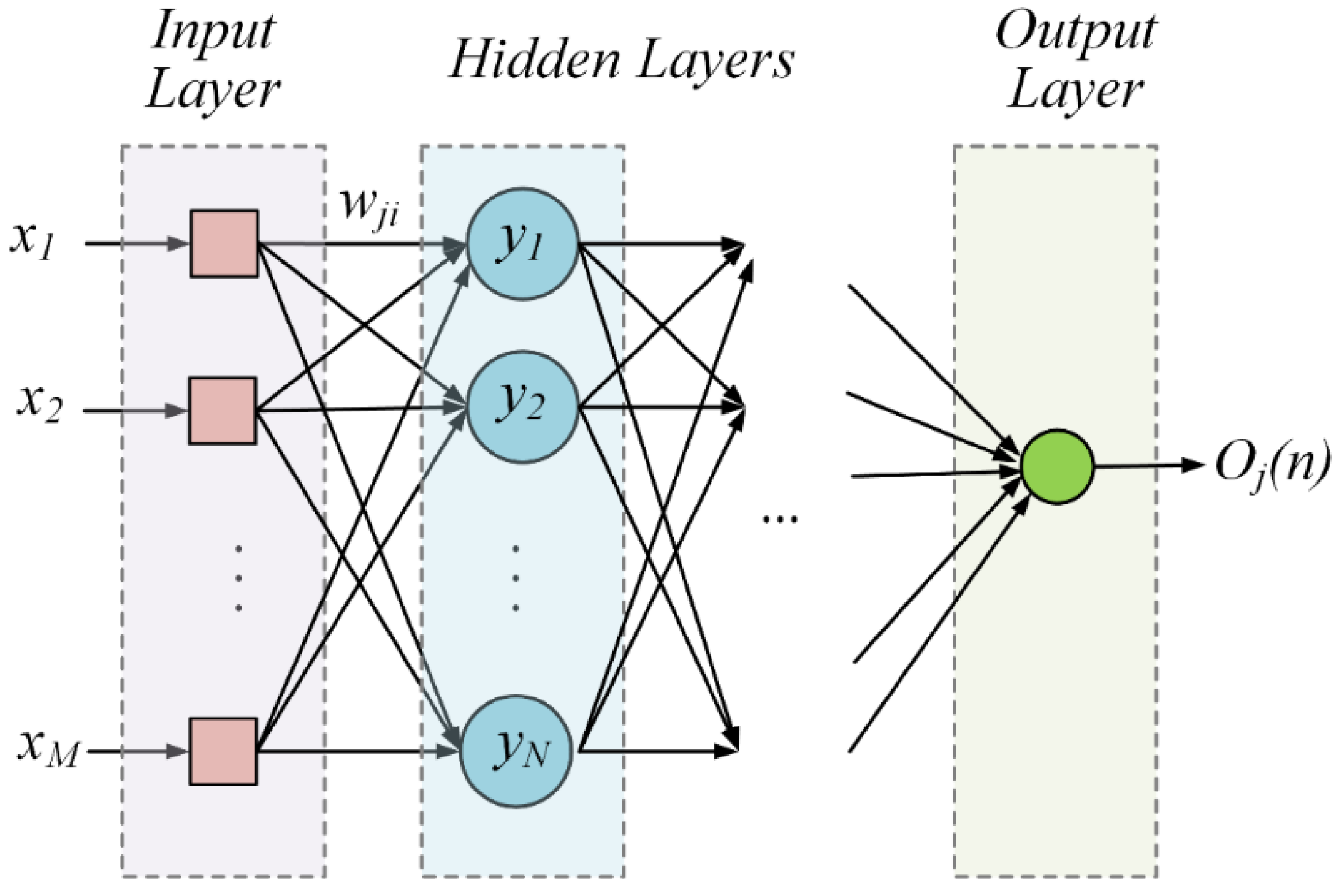
In this research, an artificial neural network (ANN) [4,27] was applied to construct the transfer model to estimate solar irradiance on tilted surfaces. A multilayer perceptron using feed-forward backpropagation was used in this work. The architecture of the ANN used in this work is illustrated in Figure 1. There are M inputs $x_1, x_2, \dots x_M$. The neurons are fully connected. The output layer has only one neuron, which corresponds to the desired output value.

To apply the ANN, the first step is to determine the network architecture, including the number of hidden layers and the number of neurons in each layer. In Figure 1, $x_i$ denotes the ith component of the input feature vector and $y_j\left(n\right)$ denotes the output of the jth neuron in the nth learning iteration. The second step of training ANN is to initialize the network, including setting the learning rate $\eta$ and the stop criteria. The third step is the feedforward stage. In the nth learning iteration, the input vector $x_i\left(n\right)$ is sent into the network. The output $y_j\left(n\right)$ of the jth neuron in the first hidden layer is computed using Equation (1). In Equation (1), the term $v_j\left(n\right)$ denotes the net internal activity level of the jth neuron in the nth learning iteration. The function $\phi (·)$ denotes the activation function of the jth neuron. The internal activity level $v_j\left(n\right)$ is computed using Equation (2). In Equation (2), P is the input dimension of the jth neuron, which does not include the threshold term. The term $w_{ji}\left(n\right)$ denotes the synaptic weights from the ith neuron to the jth neuron in the nth learning iteration. Then, the output of each layer is calculated through the hidden layers with the feedforward network.

$$y_j\left(n\right)={\phi }_j(v_j\left(n\right))$$

(1)

$$v_j\left(n\right)={\displaystyle \sum }_{i=0}^P{w}_{ji}\left(n\right)y_i\left(n\right)$$

(2)

The forth step is the back-propagation stage. The local gradient function ${\delta }_j\left(n\right)$ in the output layer in the nth learning iteration is computed using Equation (3):

$${\delta }_j\left(n\right)=e_j\left(n\right){\phi }^{\prime }(v_j\left(n\right)).$$

(3)

In Equation (3), the error term $e_j\left(n\right)$ is defined as $d_j\left(n\right)-O_j\left(n\right)$, where $d_j\left(n\right)$ is the desired output of the jth neuron in the nth learning iteration. If the activation function is a sigmoid function,$y_i\left(n\right)$ can be expressed as Equation (4):

$$y_i\left(n\right)=\frac{1}{1+\exp \left(-v_j\left(n\right)\right)} , -\infty <v_j\left(n\right)<\infty .$$

(4)

The term ${\phi }^{\prime }(v_j\left(n\right))$ can be expressed as $y_j\left(n\right)\left(1-y_j\left(n\right)\right)$. Then, the local gradient function ${\delta }_j\left(n\right)$ of each layer is calculated through back-propagating from the last hidden layer to the first hidden layer in accordance with Equation (5):

$${\delta }_j\left(n\right)={\phi }^{\prime }(v_j\left(n\right)){\displaystyle \sum }_k{\delta }_k\left(n\right)w_{kj}\left(n\right)=y_j\left(n\right)\left(1-y_j\left(n\right)\right){\displaystyle \sum }_k{\delta }_k\left(n\right)w_{kj}\left(n\right).$$

(5)

The fifth step is to adjust the synaptic weight of each neuron in accordance with Equation (6). The adjustment value to the synaptic weight $w_{ji}\left(n\right)$ in the training phase is denoted as $\Delta w_{ji}\left(n\right)$.

$$w_{ji}\left(n+1\right)=w_{ji}\left(n\right)+\Delta w_{ji}\left(n\right)=w_{ji}\left(n\right)+\mathsf{\eta }{\delta }_j\left(n\right)y_j\left(n\right)$$

(6)

The sixth step is to continue iterating the learning steps from step 3 until the stop criteria are satisfied or the number of iterations reaches the predefined maximum number of iterations.

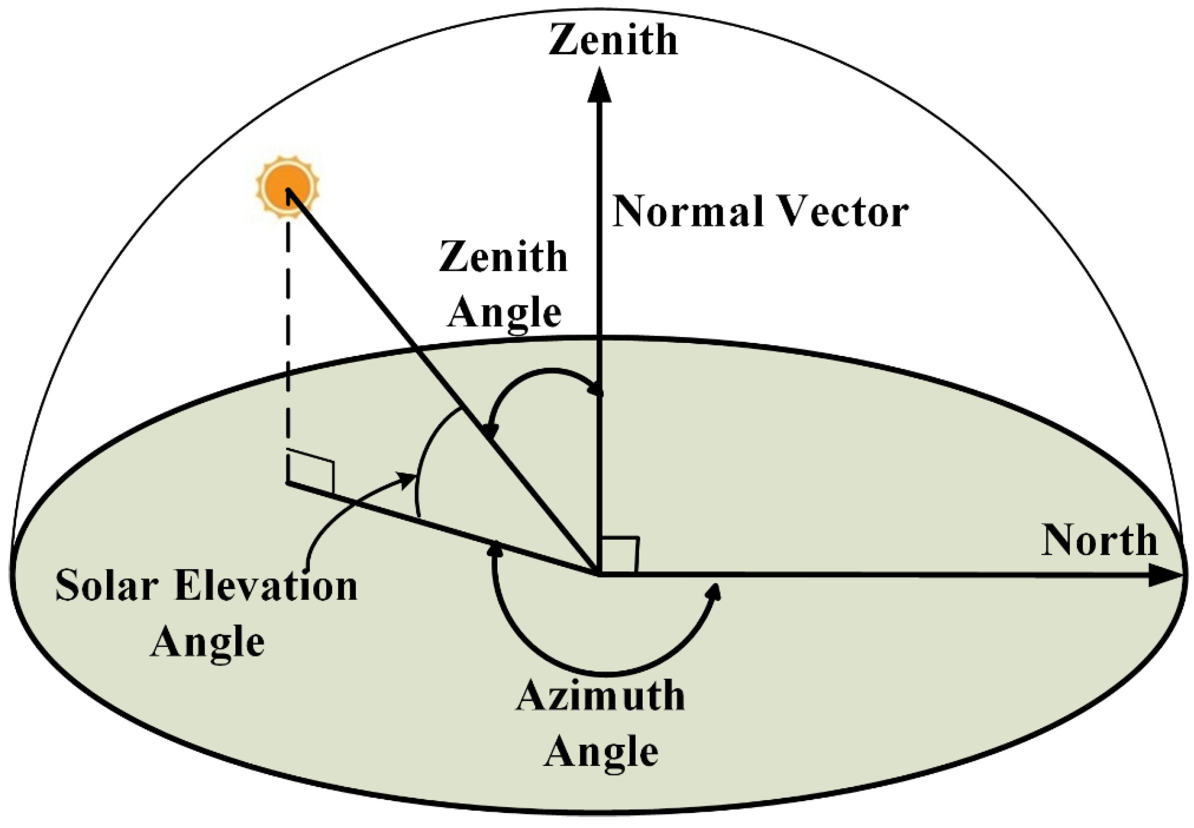
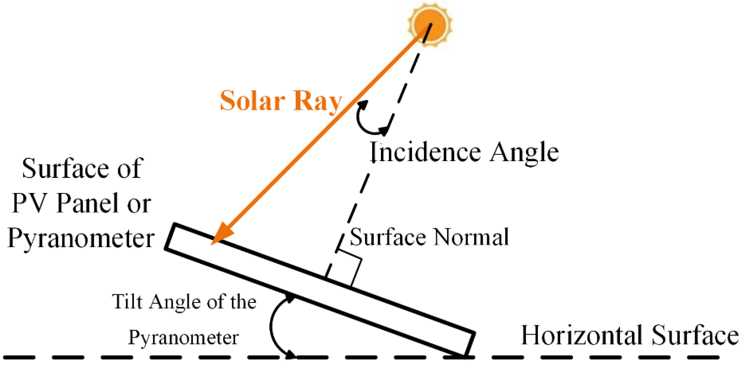
The input features of the ANN in this work include the horizontal irradiance, solar elevation angle, Cosine value of the solar azimuth angle, Sine value of the solar azimuth angle, Cosine value of the azimuth angle of the pyranometer, Sine value of the azimuth angle of the pyranometer, the tilt angle of the pyranometer, and the incidence angle of solar ray. The definitions of the solar zenith angle and the solar azimuth angle are illustrated in Figure 2. To be able to deal with tilted surfaces with arbitrary orientations and tilt angles, the azimuth angle and tilt angle of the pyranometer are also included in the input feature vector. Instead of using the angle values directly, the Cosine and Sine values are used for azimuth angles. The reason is that the azimuth angles can range from 0 to 360 degrees. Although 0 and 360 degrees are far from each other in terms of angle values, they are both describing the north direction. Therefore, expressing the azimuth angles with Cosine and Sine values can solve this problem. There is no need to express the tilt angle using Cosine and Sine values because the range of the tilt angles is practically limited to smaller values. The tilt angle of the pyranometer or the PV panel and the incidence angle of solar ray are illustrated in Figure 3. All the input features are normalized to the range of 0 to 1.

The existing works using ANN, such as that in Reference [19], estimate the inclined irradiance $\widehat{I}r{r}_{inclined}$ as the desired output in their work. However, the output of the ANN in the proposed method is the difference between the horizontal irradiance $Ir{r}_{horizontal}$ and the inclined irradiance $Ir{r}_{inclined}$, which is denoted as $\Delta Irr=Ir{r}_{horizontal}- Ir{r}_{inclined}$. Instead of predicting inclined irradiance $\widehat{I}r{r}_{inclined}$ directly, one of the main characteristics of the proposed ANN model is that the differential value $\Delta Irr$ is used as the output. The cost function of network training is based on the mean square error between $\Delta Irr$ and $\Delta \widehat{I}rr$. The estimated inclined irradiance would be the horizontal irradiance plus the output estimated differential value $\Delta \widehat{I}rr$, i.e., $\widehat{I}r{r}_{inclined}=Ir{r}_{horizontal}+ \Delta \widehat{I}rr$. We demonstrate in the experimental results that the design of differential output could reduce the estimation error.

3. Data Acquisition

Two datasets were used in the experiments. The pyranometers used to collect the datasets in the experiments are LP PYRA 03 AC. We recorded one irradiance reading per minute in the dataset. Technical characteristics of the pyranometers are listed in

Table 1. Specifications of the pyranometer.

Detailed Specifications of the Pyranometer LP PYRA 03 AC
Typical Sensitivity	10 µV/(W/m2)
Measuring Range	0~2000 W/m2
Output Signal	4~20 mA, 4 mA = 0 W/m2, 20 mA = 2000 W/m2
Impedance	33~45 Ω
Operating Temperature	−40 ℃~80 ℃
Response Time	<30 s

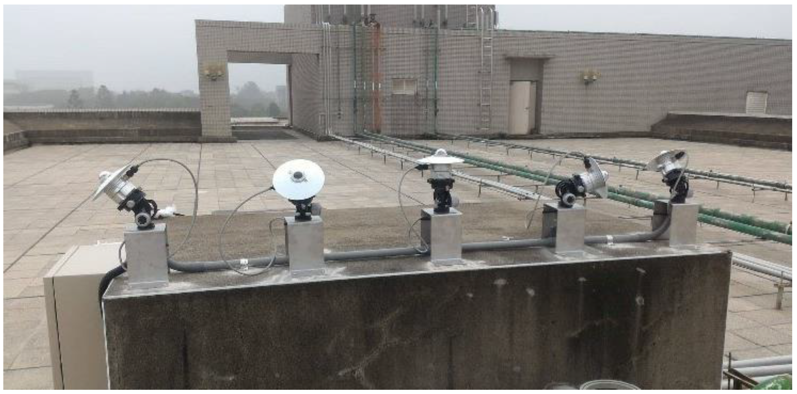
. Dataset A contains solar irradiance data of a fixed orientation and tilt angle. It includes the horizontal and tilted solar irradiance at three different locations in Taiwan for a one-year duration. The pyranometers that measured the tilted solar irradiance were with a tilt angle of 20 degrees facing south. The second dataset, dataset B, contains data of various orientations and tilt angles. 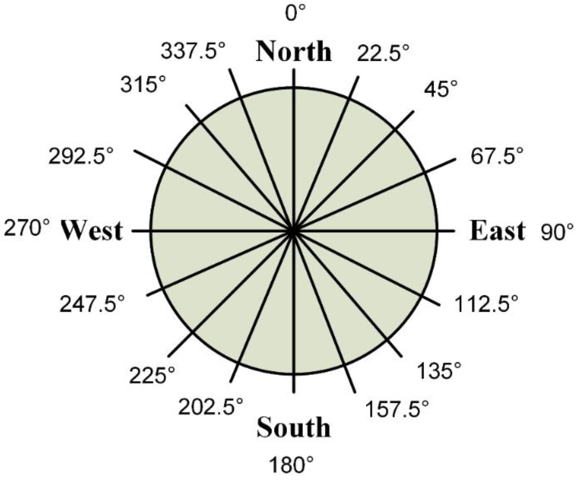To collect the second dataset, we set up five pyranometers with adjustable azimuth angles and tilt angles, as shown in Figure 4. The center pyranometer is horizontal. Each of the other four pyranometers has a tilt angle facing a certain orientation. The tilt angles and azimuth angles of these four pyranometers are adjusted periodically to specific values so that we can collect the desired experimental data. In total, there were inclined solar irradiances with four different tilt angles (10°, 15°, 20°, 30°) and sixteen different azimuth angles collected in dataset B. The sixteen azimuth angles included in dataset B are illustrated in Figure 5. For the 0-, 90-, 180-, and 270-degree orientations, the inclined pyranometers were adjusted to a 30-degree tilt angle for 20 days. The inclined pyranometers were adjusted to the other 3 tilt angles every 5 days. For all other orientation angles (other than 0°, 90°, 180°, and 270°), the inclined pyranometers were adjusted to each of the four tilt angles every 5 days. After collecting data for all the tilt angles of an orientation, the pyranometers were adjusted to a new orientation angle. With four inclined pyranometers, we can collect four orientations at the same time. It takes 95 days for one rotation. The process of rotation took place 3 times, taking 285 days. The data were collected from 08:00 to 17:00 for 9 h and recorded each minute. Therefore, there were 540 data points collected in a day. For a 30-degree tilt angle of 0, 90, 180, 270-degree orientations, we have 60-day data with 32,400 data points. For all other angle combinations, we have 15-day data with 8100 data points for each angle combination. Note that the horizontal pyranometer has all the data for a 0-degree tilt angle throughout the entire data collection period.

4. Experimental Results

We used Dataset A and Dataset B described in the previous section to evaluate the proposed framework. The results on Dataset A and Dataset B are elaborated in Section 4.1 and Section 4.2, respectively. In the experiments, we used the network with three hidden layers. Each hidden layer has six neurons. The evaluation metrics of the estimation results are mean absolute percentage error (MAPE) and root mean square percentage error (RMSPE) as shown in Equations (7) and (8), respectively. Mean absolute error measures the absolute difference between the ground truth inclined irradiance $Ir{r}_{inclined}$ and the estimated inclined irradiance $\widehat{I}r{r}_{inclined}$. Root mean square error is the square root of the average of squared errors. Both of these error metrics are presented in terms of percentage in contrast to the original ground truth values. In Equations (7) and (8), Num denotes the number of data samples being evaluated. The time scale of the metrics is one minute.

$$\mathrm{MAPE}=\frac{{{\displaystyle \sum }}_{k=1}^{Num}\left|Ir{r}_{inclined}\left(k\right)-\widehat{I}r{r}_{inclined}\left(k\right)\right|}{{{\displaystyle \sum }}_{k=1}^{Num}Ir{r}_{inclined}\left(k\right)}\times 100\%$$

(7)

$$RMSP{E}_{fc}=\frac{\sqrt{\frac{1}{Num}{{\displaystyle \sum }}_{k=1}^{Num}{\left(Ir{r}_{inclined}\left(k\right)-\widehat{I}r{r}_{inclined}\left(k\right)\right)}^2}}{\frac{1}{Num}{{\displaystyle \sum }}_{k=1}^{Num}Ir{r}_{inclined}\left(k\right)}\times 100\%$$

(8)

4.1. Results on Dataset A

Dataset A was used to test the accuracy of the transfer model for the training and testing data with a fixed orientation and tilt angle. The purpose of Dataset A is to show that the design of differential output values could reduce the estimation error compared with existing ANN transfer models. If horizontal and tilted irradiance data of two or more years are available, it is suggested that the data of one year are used for training and the data of the following years are used for testing. Since the solar elevation angle, the solar azimuth angle, and the incidence angle of solar ray would exhibit a different relationship in different months of a year, it would be better to construct a model in January and use the model to test the data in January in the following years. However, in this case, it would require collecting measurement data for a whole year before the system can be deployed. In cases where the training data are limited in the initial deployment phase, a solution is to use the training data from the previous month to construct a model and apply the transfer model to obtain tilted irradiance in the following month. This solution helps with faster deployment with limited data. To further analyze the influence of the time period of the training data used to construct the transfer model, we divided the experiments on dataset A into two parts. The first experiment on dataset A used a fixed time distance between the training and testing data. The second experiment on dataset A considered various time distances between the training and testing data and observed their impact on the estimation accuracy. Note that the experiments on Dataset A train separate models for separate locations.

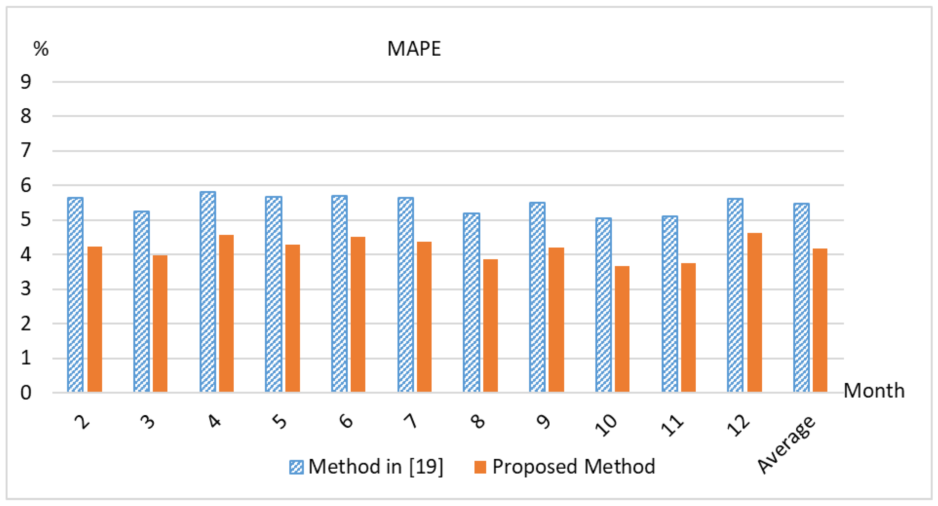
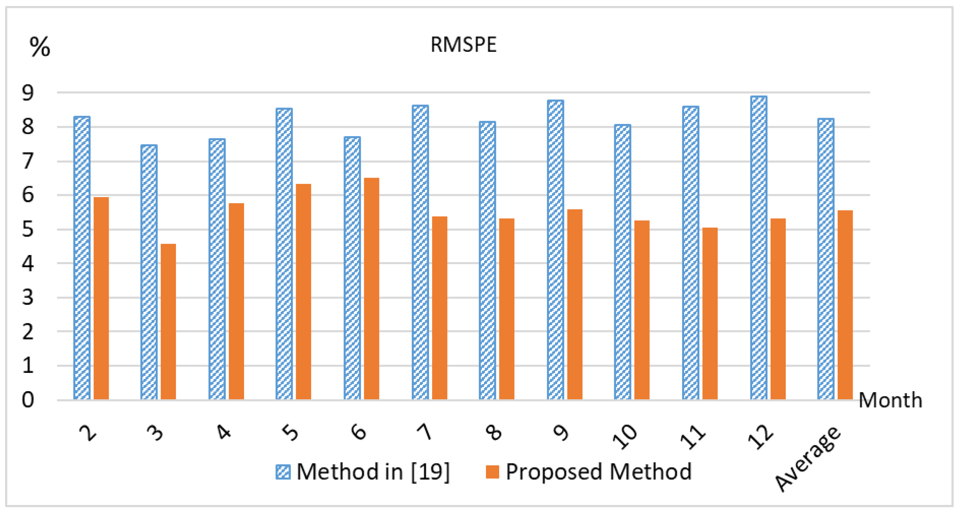
For the first experiment on dataset A, the samples in each month were tested using the ANN model constructed by the data from the previous month. For example, the data of February were tested using the transfer model constructed by the data of January. The data of March were validated using the transfer model trained by the data of February. The estimation MAPE and RMSPE on dataset A using data from the previous month as training data are shown in Figure 6 and Figure 7, respectively. The MAPE and RMSPE of the proposed method and the method in Reference [19] are compared. The settings of the ANN implementation in Reference [19] are the same as the best parameters recommended in Reference [19]. We can observe that the proposed method exhibits lower error in terms of both MAPE and RMSPE compared with Reference [19]. The main reason is that the range of the difference between the horizontal and inclined irradiance is much smaller than the range of inclined irradiance. Therefore, the design of the proposed method helps to reduce estimation errors.

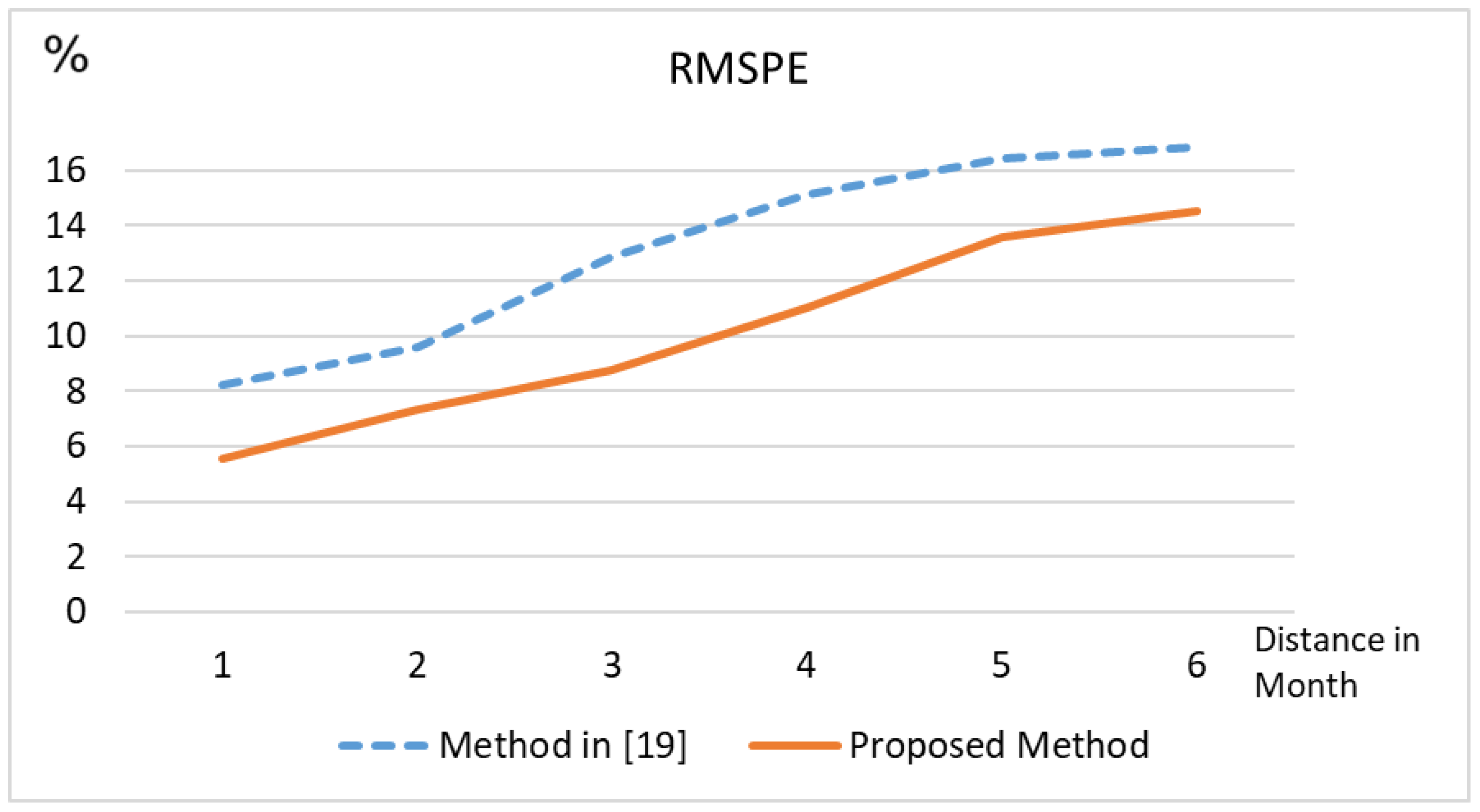
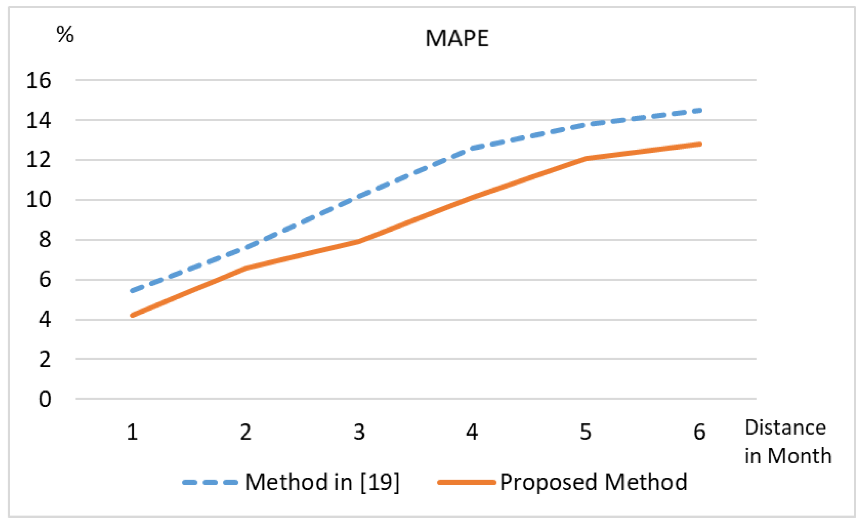
For the second experiment on dataset A, we used training and testing data from various time periods. The estimation MAPE and RMSPE on dataset A using training and testing data with different distances are shown in Figure 8 and Figure 9, respectively. In Figure 8 and Figure 9, the x axis represents the time distance between the training and testing data. The unit of the time distance is month. For example, if the transfer model constructed by the data of February is used to estimate the inclined irradiance of March, the time distance between the training and testing data is one month. If the transfer model constructed by the data of January is used to estimate the inclined irradiance of March, the time distance between the training and testing data is two months. Notice that the time distance between January and December is one instead of eleven. The maximum time distance between the training and testing data is six. We can observe that the error of estimation increases as the time distance becomes larger. Therefore, it is recommended that the time distance between the training and testing data should not be too large. In practice, a transfer model can be constructed each month. The transfer model can be used to obtain the estimated inclined irradiance of the succeeding month.

4.2. Results on Dataset B

Dataset B was used to validate the proposed transfer model when the tilt and azimuth angles were not in the training set. As described in Section 3, Dataset B contains irradiance data of four different tilt angles (10°, 15°, 20°, 30°) and sixteen different azimuth angles. To establish the transfer model, the training data are listed in

Table 2. Training data.

Azimuth Angle	Tilt Angle
-	0°
0°	30°
90°	30°
180°	30°
270°	30°

. The horizontal irradiance is regarded as training data with a zero-degree tilt angle. In the experiments, we used inclined irradiance of 0 and 30 degrees as the training samples in order to infer inclined irradiance of all the other tilt angles between 0 and 30 degrees. We used training data of four orthogonal azimuth angles to infer the inclined irradiance of all the other azimuth angles in the testing data. The combinations of the four tilt angles and sixteen azimuth angles in the testing data are shown in

Table 3. Testing data.

Azimuth Angles of Pyranometers	Tilt Angle
0°	10°, 15°, 20°
90°	10°, 15°, 20°
180°	10°, 15°, 20°
270°	10°, 15°, 20°
22.5°	10°, 15°, 20°, 30°
45°	10°, 15°, 20°, 30°
67.5	10°, 15°, 20°, 30°
112.5°	10°, 15°, 20°, 30°
135°	10°, 15°, 20°, 30°
157.5	10°, 15°, 20°, 30°
202°	10°, 15°, 20°, 30°
225°	10°, 15°, 20°, 30°
247.5°	10°, 15°, 20°, 30°
292.5°	10°, 15°, 20°, 30°
315°	10°, 15°, 20°, 30°
337.5°	10°, 15°, 20°, 30°

.

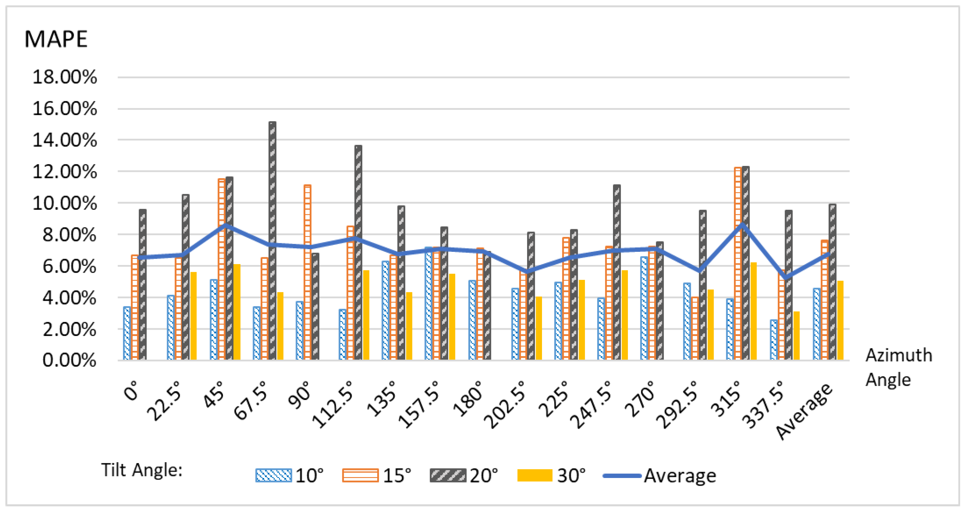
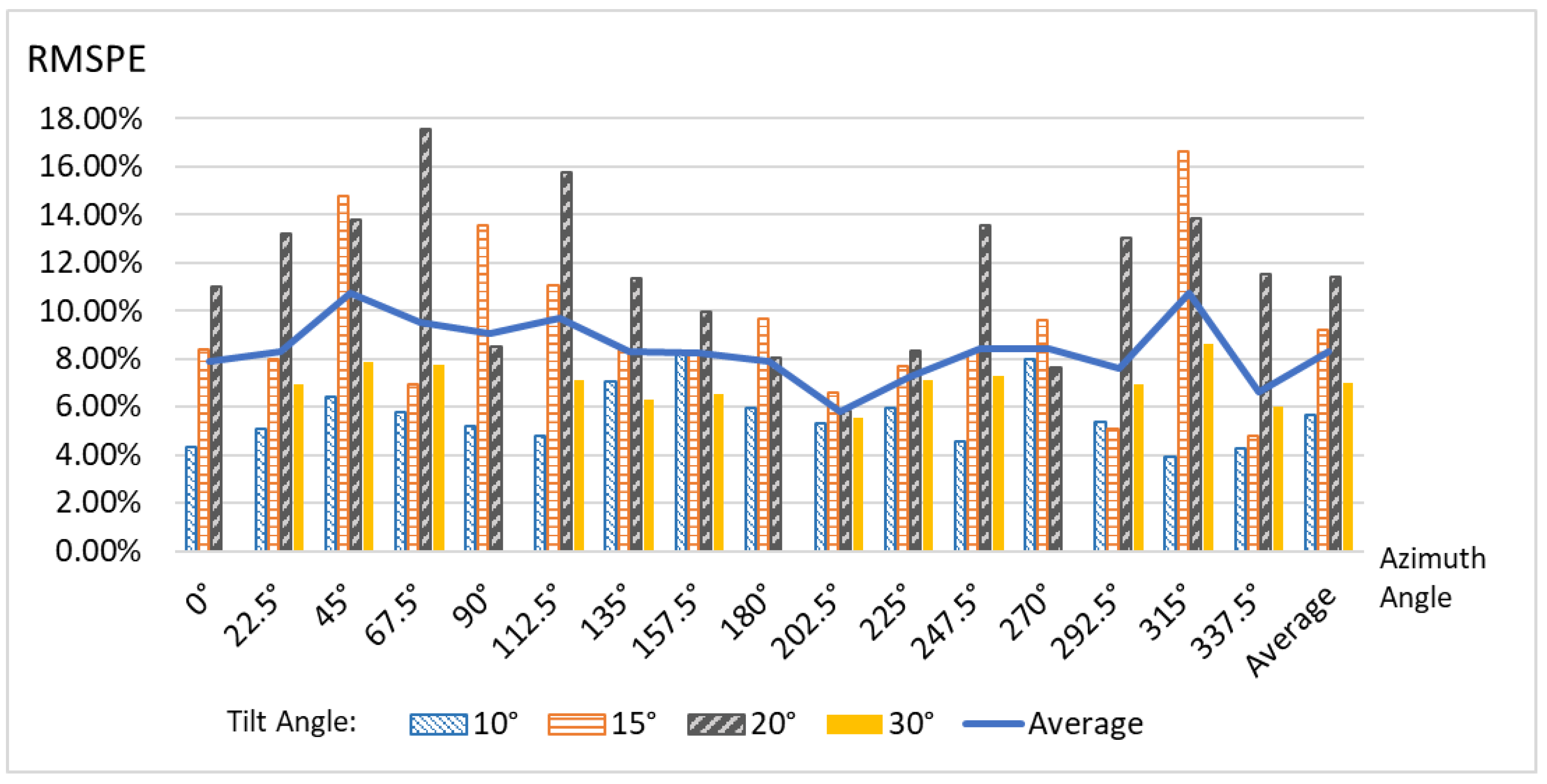
The purpose of the experiments on dataset B is to show that although the tilt angles and azimuth angles are not included in the training data, the trained model can still successfully estimate the inclined irradiance of all the tilt angles and azimuth angles in the testing data with a low error rate. The MAPE and RMSPE of estimated inclined irradiance on dataset B are shown in Figure 10 and Figure 11, respectively. Note that the samples of 30-degree tilt angles on the four orthogonal orientations 0°, 90°, 180°, 270° are not evaluated because these angle combinations are included in the training data. The overall averaged MAPE and RMSPE on dataset B are 6.79% and 8.02%, respectively. From the experimental results, we can observe that using horizontal irradiance and 30-degree inclined irradiance in the four orthogonal directions as training data, the established model can estimate inclined irradiance with arbitrary azimuth angles and tilt angles between 0 to 30 degrees.

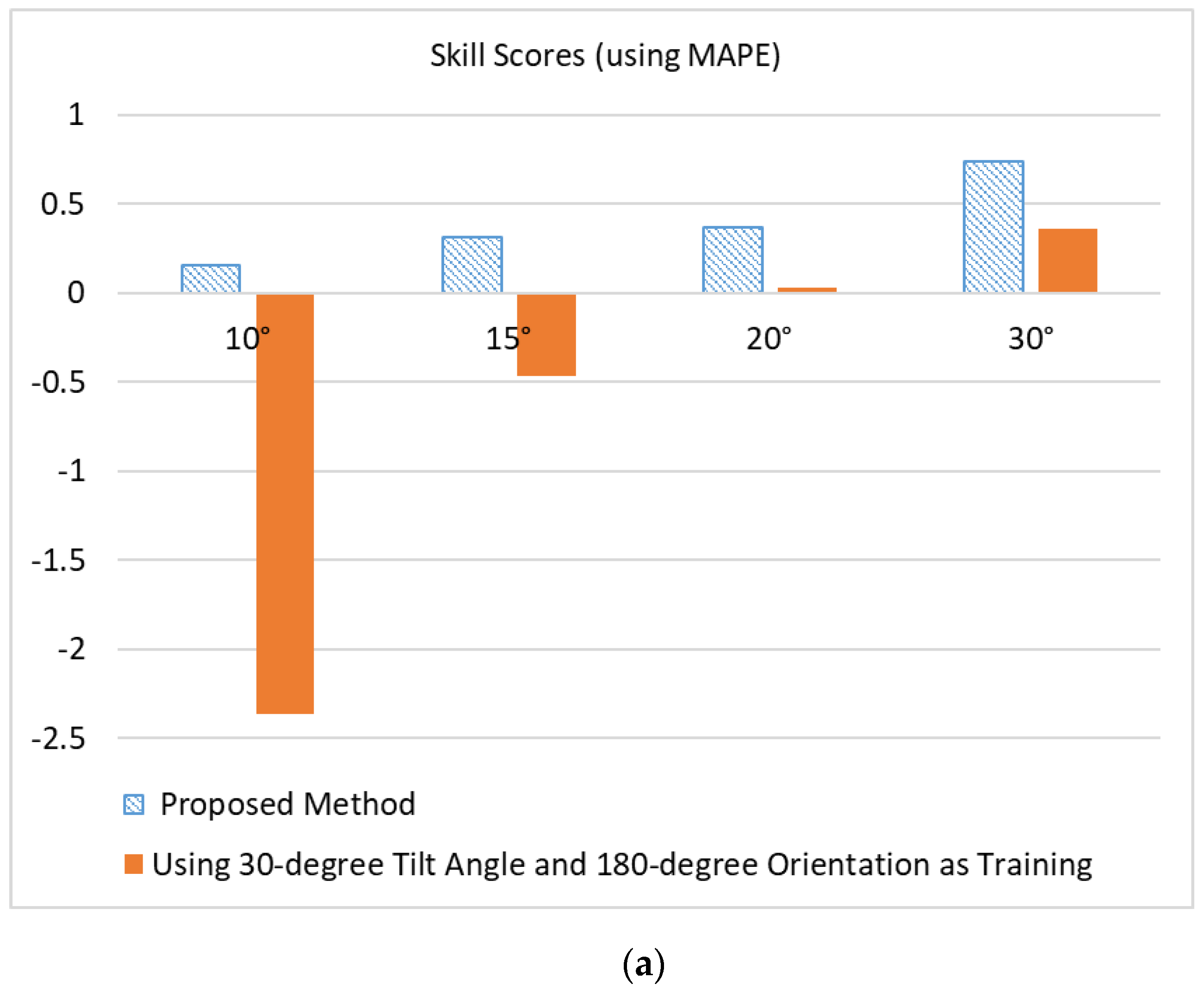
To further evaluate the effectiveness of the proposed method, we compared the proposed method with a baseline method using the skill score (SS) [28] metrics defined in Equation (9). A method is better than the baseline method if the skill score is positive. The degree of improvement is better when the skill score is closer to one.

$$S{S}_{MAPE}=1- \frac{MAP{E}_{proposed}}{MAP{E}_{baseline}} , S{S}_{RMSPE}=1- \frac{RMSP{E}_{proposed}}{RMSP{E}_{baseline}}$$

(9)

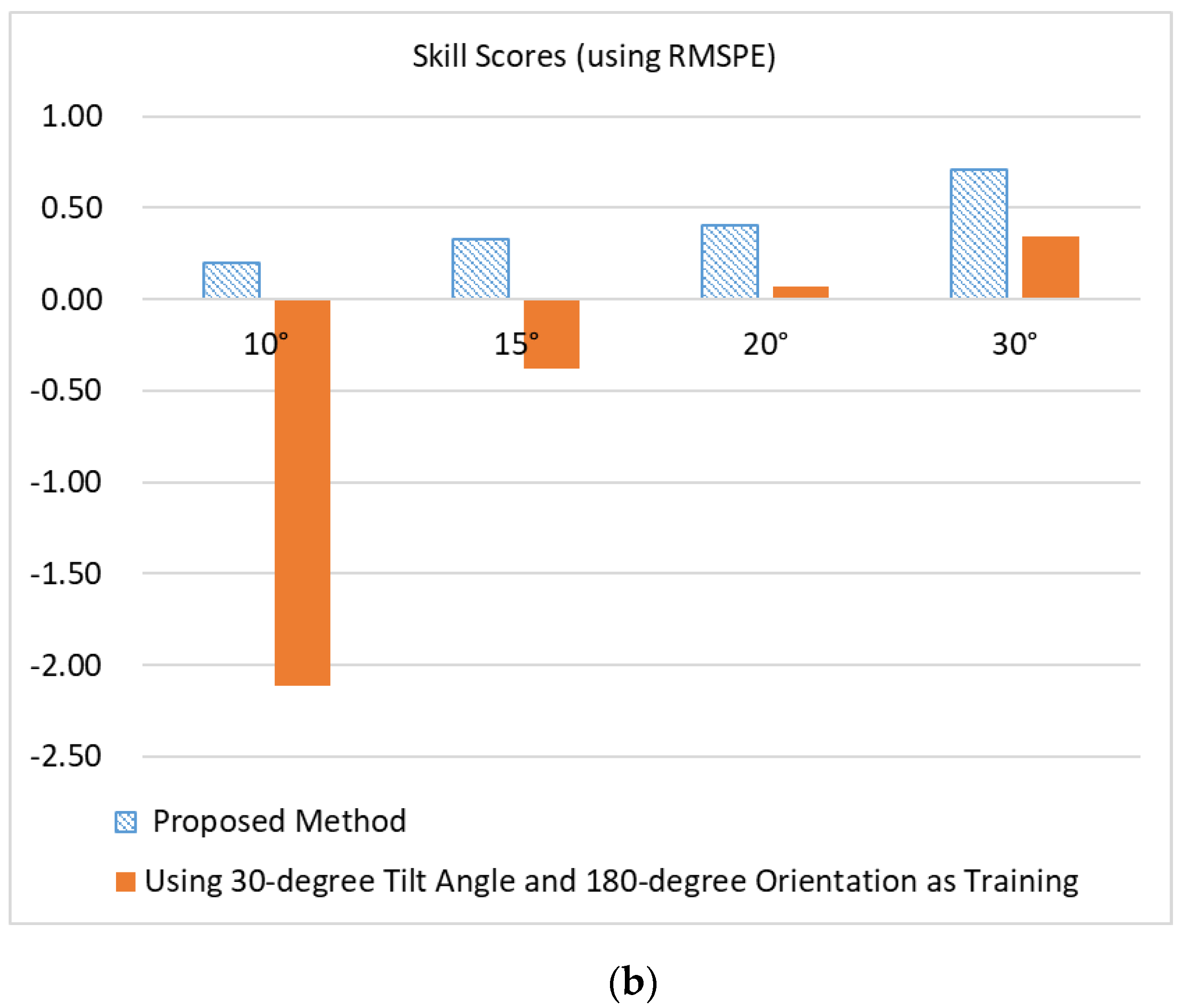
Existing methods that construct transfer models via training such as those in References [18,19,20,21] cannot estimate inclined irradiance for tilt and orientation angles that are not included in the training dataset using a unified transfer model. Therefore, for dataset B, we compared the proposed method with a baseline method that uses horizontal irradiance as the estimation result. The $S{S}_{MAPE}$ and $S{S}_{RMSPE}$ are illustrated in Figure 12. We can observe that the skill scores of the proposed method are positive under all conditions. As the tilt angle becomes larger, the proposed method exhibits better skill scores in contrast to the baseline. This means that the proposed transfer model has more obvious improvement when the difference between the horizontal irradiance and the inclined irradiance is larger. Furthermore, we calculated the skill scores of Reference [19] on dataset B using a 30-degree tilt angle and 180-degree orientation as training data. We denoted the model trained by the 30-degree tilt angle and 180-degree orientation as M_f. Since model M_f is trained using a 30-degree tilt angle and there is no input feature regarding the tilt angle of the inclined surface, it exhibits high MAPE for 10-degree and 15-degree tilt angle testing data. The MAPE of M_f on 10-degree and 15-degree tilt angle testing data is much higher than the baseline. Recall that the baseline uses horizontal irradiance as the estimation result. Therefore, the MAPE of baseline on 10-degree and 15-degree tilt angle testing data is relatively low. As a result, the skill scores of model M_f on these two tilt angles are negative. For 20-degree and 30-degree tilt angle testing data, model M_f yields better results than the baseline since the testing tilt angles are closer to the training tilt angles. However, since model M_f is trained with data from only one fixed orientation, it still cannot yield satisfying accuracy when the test data are collected using various orientations. As a consequence, the skill scores of the proposed method are still much higher than those of model M_f on 20-degree and 30-degree tilt angle testing data.

5. Conclusions

In this work, artificial neural networks were utilized to construct the transfer model to estimate solar irradiance on tilted surfaces. Instead of predicting tilted irradiance directly, the proposed method estimated the differences between the horizontal irradiance and the irradiance on a tilted surface. The range of the difference between the horizontal and inclined irradiance was much smaller than the range of inclined irradiance. If we estimated the difference, it would prevent the estimated inclined irradiance drift too far away from the ground truth. The outputs of the proposed ANNs were differential values. According to the experiments, the design of differential output can help to enhance the estimation accuracy. The experiments also analyze the estimation accuracy using different time distances between the training and testing data. Two datasets were tested in the experiments. First, for the dataset with a fixed orientation and tilt angle, the proposed method can successfully estimate inclined solar irradiance with a lower error compared to existing methods. Second, for the dataset with various orientations and tilt angles, using horizontal irradiance and inclined irradiance of a tilt angle θ as training data, the transfer model can infer the inclined irradiance of any tilt angles between 0 and θ although those tilt angles are not included in the training data. Further, using inclined irradiance at four orthogonal orientations as training data, the transfer model can estimate the inclined irradiance of arbitrary orientations. It was validated that the trained model can successfully estimate inclined irradiance of arbitrary orientations and tilt angles in the testing data with satisfactory accuracy.