Mixed Integer Quadratic Programming Based Scheduling Methods for Day-Ahead Bidding and Intra-Day Operation of Virtual Power Plant

Abstract
:1. Introduction
- (1)
- A scheduling method for DA market bidding: The method considers the maximization of VPP revenue with a 1 h step.
- (2)
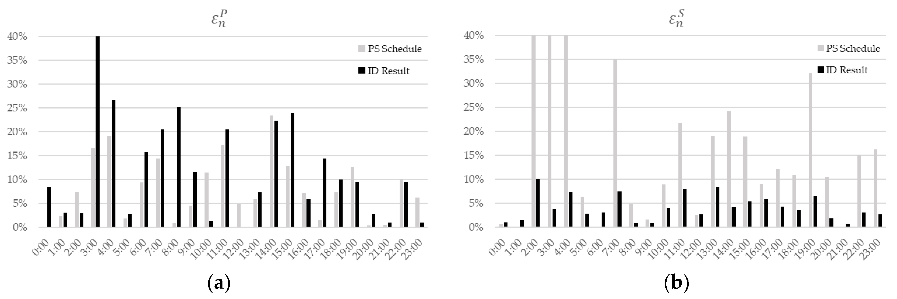
- A rescheduling method for ID operation: The method considers the minimization of the hourly generation error and 5 min generation variation with a 5 min scale.
2. Market Environment and Scheduling Scheme
2.1. Market Environment
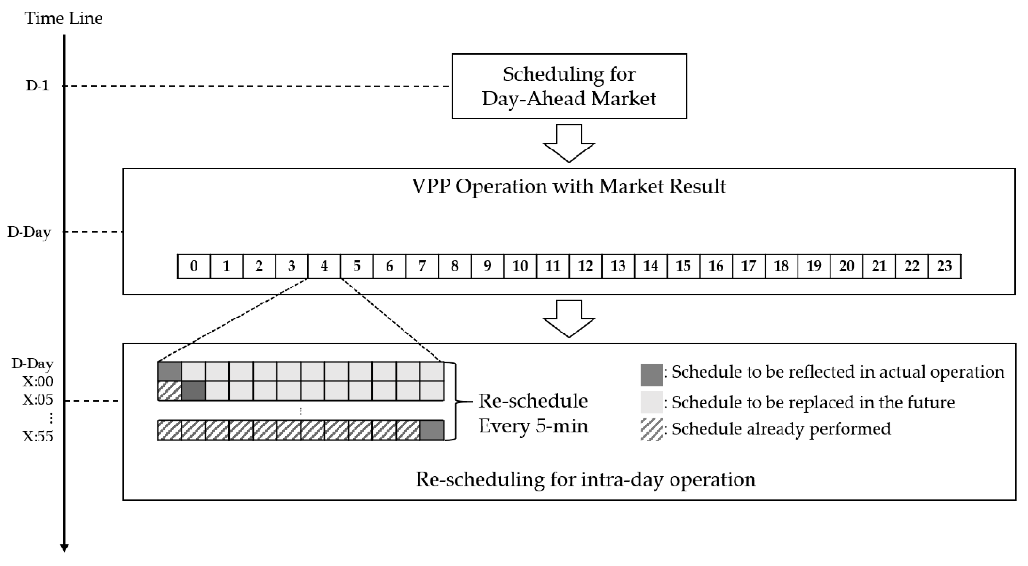
2.2. Scheduling Scheme
3. Scheduling Methods for DA Market Bidding and ID Operation
3.1. Scheduling Method for DA Market Bidding
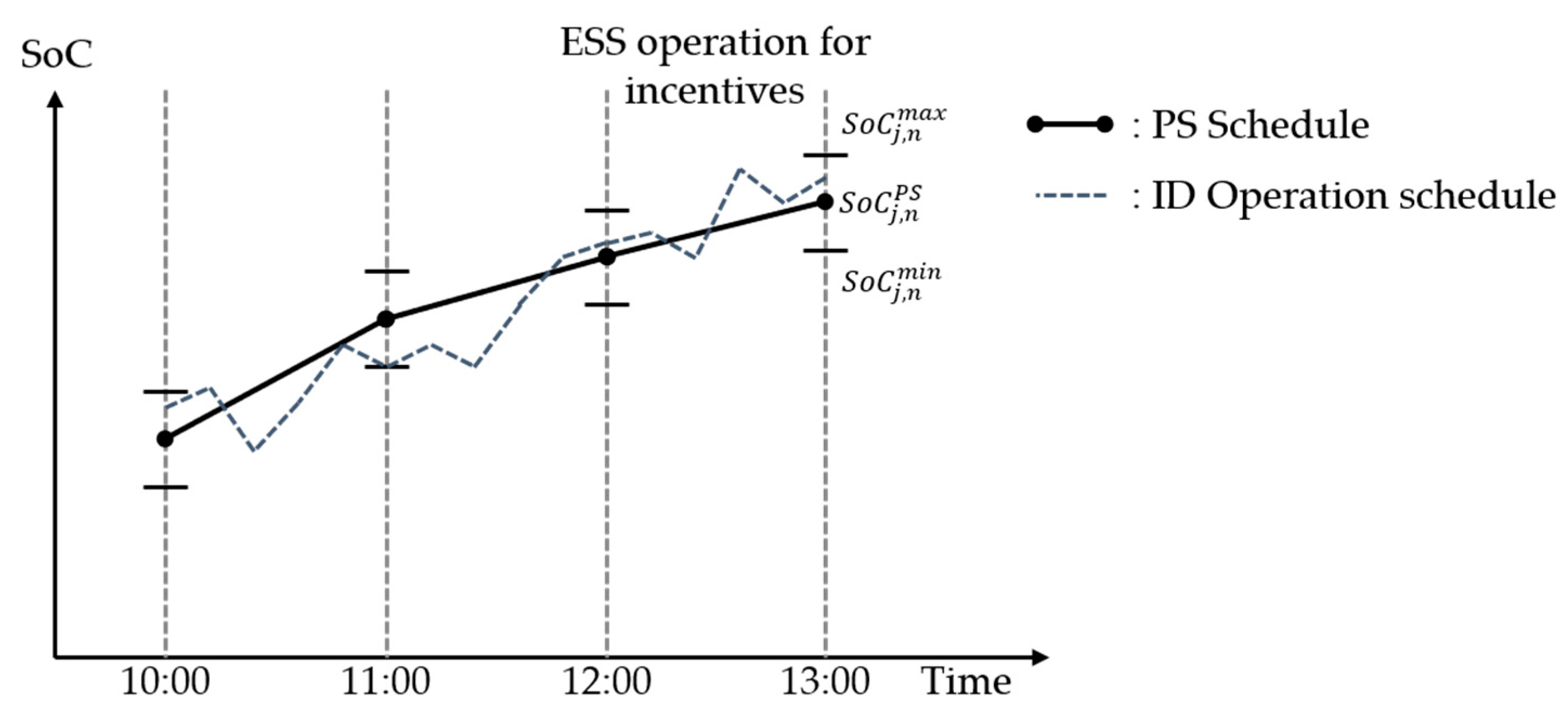
3.2. Scheduling Method for ID Operation
4. Numerical Result
4.1. Numerical Result for DA Market Bidding
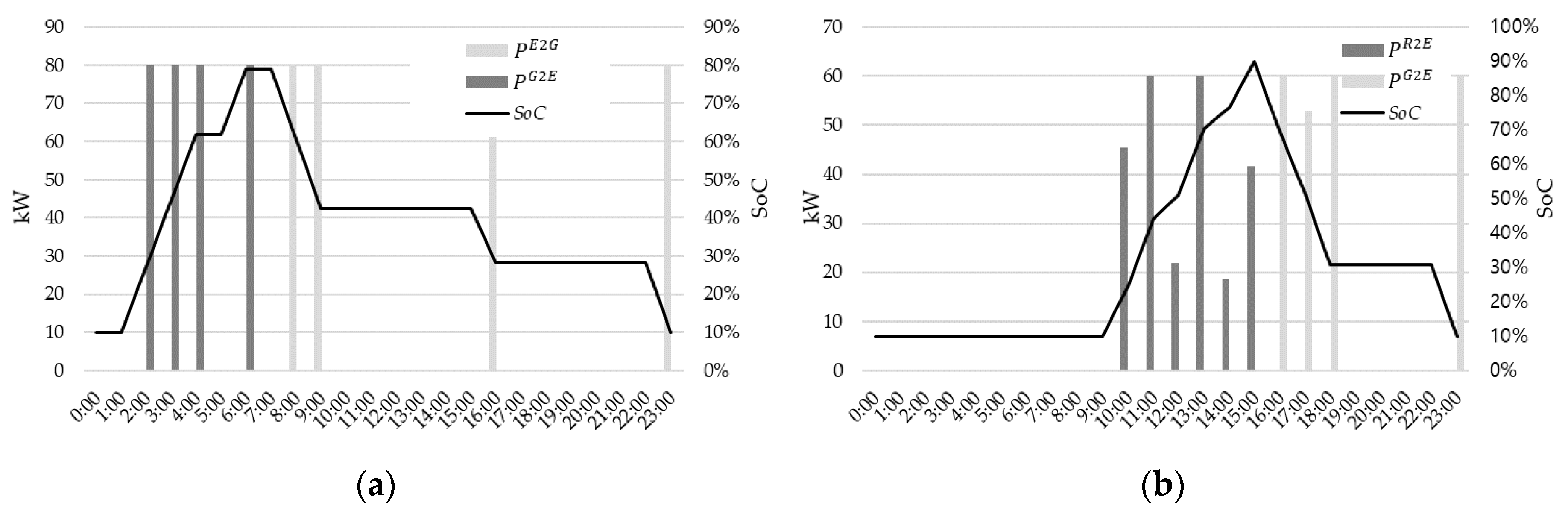
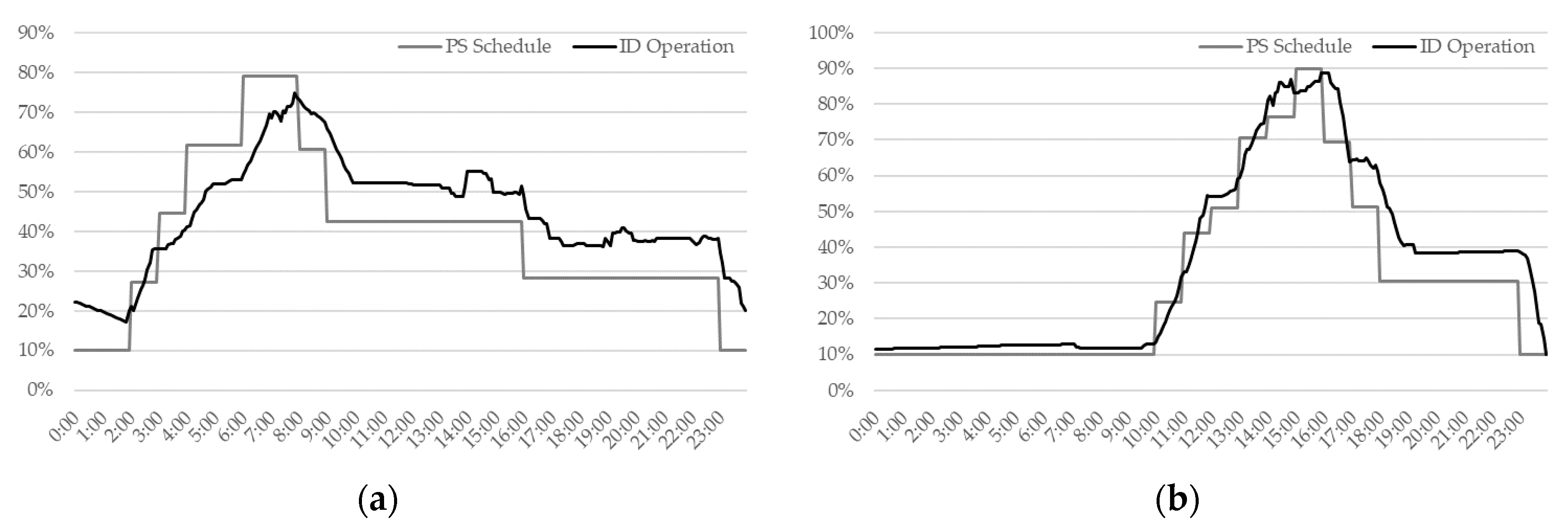
4.2. Numerical Result for ID Operation
5. Conclusions
Author Contributions
Acknowledgments
Conflicts of Interest
Acronyms
| VPP | Virtual Power Plant |
| MIQP | Mixed Integer Quadratic Programming |
| DA | Day-Ahead |
| ID | Intra-Day |
| SMP | System Marginal Price |
| REC | Renewable Energy Certification |
| AGC | Automatic Generation Control |
| DER | Distributed Energy Resource |
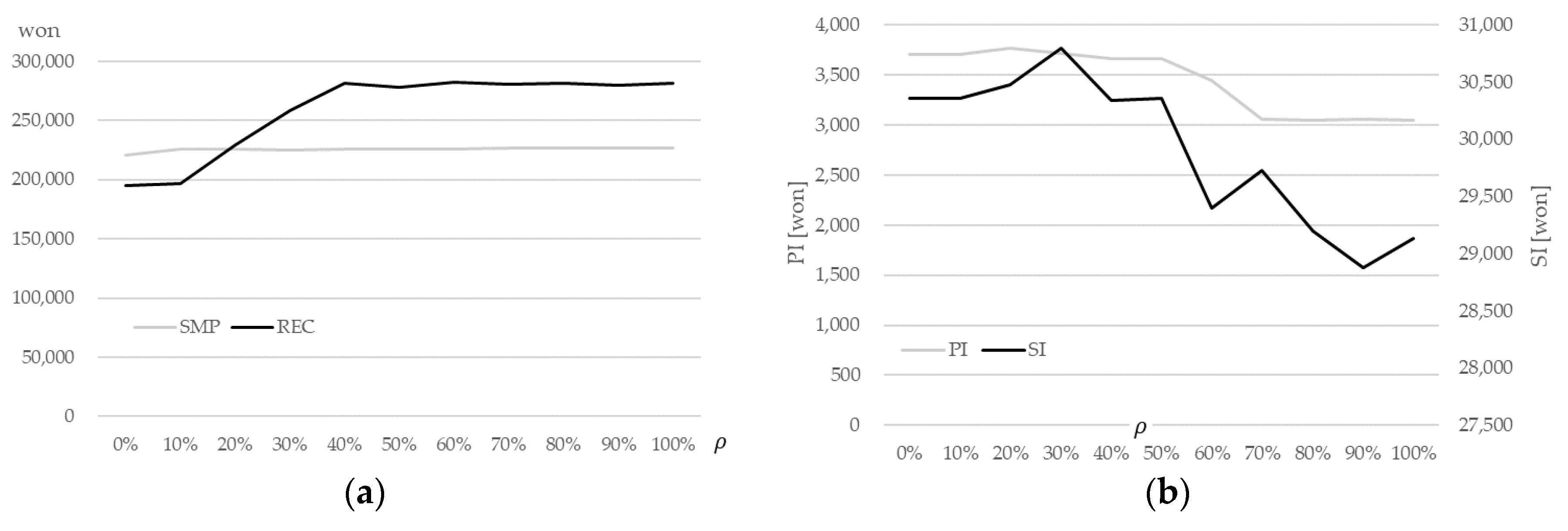
| PI | Predictability Incentive |
| SI | Stability Incentive |
| RES | Renewable Energy Source |
| PV | Photovoltaic |
| WT | Wind Turbine |
| ESS | Energy Storage System |
| DG | Distributed Generators |
| PS | Previously Set |
| PCS | Power Conversion System |
Nomenclature
| Predictable incentive in n-th hour (₩) | |
| Stability incentive in n-th hour (₩) | |
| Relative difference between bid and actual generation at the n-th hour (%) | |
| Average relative difference between the generation at two adjacent times at the n-th hour (%) | |
| Binary variable equal to 1 if only is larger than 0.3 (30%) at the n-th hour | |
| Binary variable equal to 1 if only is larger than 0.3 (30%) at the n-th hour | |
| AGC price for traditional generators at the n-th hour (₩/kW) | |
| Capacity price for traditional generators at the n-th hour (₩/kW) | |
| Net generation of VPP at the n-th hour (kW) | |
| SMP at time t (₩/kWh) | |
| Given REC with 1 weight in a day | |
| Given REC with 5 weight in a day | |
| REC price (₩) | |
| Net generation of VPP at the time t (kW) | |
| is the history of (kW) | |
| Bid at the n-th hour (kW) | |
| Generation of RES i at time t (kW) | |
| , | Discharged power (ESS to Grid) of ESS j, k at time t (kW) |
| Charged power (Grid to ESS) of ESS j at time t (kW) | |
| Charged power (Renewable to ESS) of ESS j at time t (kW) | |
| , | Maximum discharging powers of ESS j and k (kW) |
| , | Maximum charging powers of ESS j and k (kW) |
| , | Binary variable, which equals 1 if there is a state change of ESS j, k at time t |
| , | Binary variables, which are equal to 1 only if ESS j or k is discharging at time t |
| , | Limit coefficient of charging and discharging of ESS j, k |
| , | Efficiency of PCS in ESS j, k (%) |
| , | SoC of ESS j, k at time t (%) |
| , | Lower bound of SoC of the ESS j, k (%) |
| , | Upper bound of SoC of the ESS j, k (%) |
| , | Capacity of ESS j, k (kWh) |
| , | SoC lower bound of ESS j, k at the n-th hour (%) |
| , | Upper bound of ESS j, k at the n-th hour (%) |
| , | Penalty for the state change of ESS j, k (₩) |
| Generation of DG l at time t (kW) | |
| Maximum generation of DG l (kW) | |
| Binary variable equal to 1 only if DG l is generating at time t | |
| Cost function of DG l (₩) | |
| Coefficient of cost function of DG l (₩/(kW)2) | |
| Coefficient of cost function of DG l (₩/kW) | |
| Coefficient of cost function of DG l (₩) | |
| Pre-Scheduled generation of DG l, at the n-th hour (kW) | |
| Very first time, which is considered re-scheduling |
References
- Safdaria, A.; Fotuhi-Firuzabad, M.; Lehtonen, M.; Aminifar, F. Optimal Electricity Procurement in Smart Grids with Autonomous Distributed Energy Resources. IEEE Trans. Smart Grid 2015, 6, 2975–2984. [Google Scholar] [CrossRef]
- Karim, M.E.; Munir, A.B.; Karim, M.A.; Muhammad-Sukki, F.; Abu-Bakar, S.H.; Sellami, N.; Bani, N.A.; Hassan, M.Z. Energy Revolution for Our Common Future: An Evaluation of the Emerging International Renewable Energy Law. Energies 2018, 11, 1769. [Google Scholar] [CrossRef]
- Mazzeo, D.; Oliveti, G.; Baglivo, C.; Congedo, P.M. Energy reliability-constrained method for the multi-objective optimization of a photovoltaic-wind hybrid system with battery storage. Energy 2018, 156, 688–708. [Google Scholar] [CrossRef]
- Kong, J.; Lee, W.; Jung, J. Economic Analysis for the Existing PV Supplier to Decide Whether to Install ESS or Not in South Korea. In Proceedings of the IEEE Innovative Smart Grid Technologies—Asia, Singapore, 22–25 May 2018. [Google Scholar]
- Pudjianto, D.; Ramsay, C.; Strbac, G. Virtual power plant and system integration of distributed energy resources. IET Renew. Power Gener. 2007, 1, 10–16. [Google Scholar] [CrossRef]
- Park, Y.-G.; Park, J.-B.; Kim, N.; Lee, K.Y. Linear Formulation for Short-Term Operational Scheduling of Energy Storage Systems in Power Grids. Energies 2017, 10, 207. [Google Scholar] [CrossRef]
- Metza, D.; Saraiva, J.T. Use of battery storage systems for price arbitrage operations in the15- and 60-min German intraday markets. Energy 2018, 160, 27–36. [Google Scholar]
- Aloini, D.; Crisostomi, E.; Raugi, M.; Rizzo, R. Optimal Power Scheduling in a Virtual Power Plant. In Proceedings of the 2011 2nd IEEE PES International Conference and Exhibition on Innovative Smart Grid Technologies, Manchester, UK, 5–7 December 2011. [Google Scholar]
- Xie, J.; Cao, C. Non-Convex Economic Dispatch of a Virtual Power Plant via a Distributed Randomized Gradient-Free Algorithm. Energies 2017, 10, 1051. [Google Scholar] [CrossRef]
- Kardakos, E.G.; Simoglou, C.K.; Bakirtzis, A.G. Optimal Offering Strategy of a Virtual Power Plant: A Stochastic Bi-Level Approach. IEEE Trans. Smart Grid 2016, 7, 794–806. [Google Scholar] [CrossRef]
- Bakari, K.E.; Kling, W.L. Development and operation of virtual power plant system. In Proceedings of the 2011 2nd IEEE PES International Conference and Exhibition on Innovative Smart Grid Technologies, Manchester, UK, 5–7 December 2011. [Google Scholar]
- Wang, Y.; Ai, X.; Tan, Z.; Yan, L.; Liu, S. Interactive Dispatch Modes and Bidding Strategy of Multiple Virtual Power Plants Based on Demand Response and Game Theory. IEEE Trans. Smart Grid 2016, 7, 510–519. [Google Scholar] [CrossRef]
- Han, H.; Cui, H.; Gao, S.; Shi, Q.; Fan, A.; Wu, C. A Remedial Strategic Scheduling Model for Load Serving Entities Considering the Interaction between Grid-Level Energy Storage and Virtual Power Plants. Energies 2018, 11, 2420. [Google Scholar] [CrossRef]
- Soysal, E.R.; Olsen, O.J.; Skytte, K.; Sekamane, J.K. Intraday market asymmetries—A Nordic example. In Proceedings of the 2017 14th International Conference on the European Energy Market (EEM), Dresden, Germany, 6–9 June 2017. [Google Scholar]
- Saez-de-Ibarra, A.; Milo, A.; Gaztañaga, H.; Debusschere, V.; Bacha, S. Co-Optimization of Storage System Sizing and Control Strategy for Intelligent Photovoltaic Power Plants Market Integration. IEEE Trans. Sustain. Energy 2016, 7, 1749–1761. [Google Scholar] [CrossRef]
- Chu, L.; Zhou, F.; Guo, J. Investigation of cycle life of li-ion power battery pack based on LV-SVM. In Proceedings of the 2011 International Conference on Mechatronic Science, Electric Engineering and Computer (MEC), Jilin, China, 19–22 August 2011. [Google Scholar]
- Yang, T.; Wu, D.; Stoorvogel, A.A.; Stoustrup, J. Distributed coordination of energy storage with distributed generators. In Proceedings of the 2016 IEEE Power and Energy Society General Meeting (PESGM), Boston, MA, USA, 17–21 July 2016. [Google Scholar]


| Name | (%) | ||||||
|---|---|---|---|---|---|---|---|
| ESS1 (Combined) | 150 | 150 | 300 kWh | 10 | 90 | 98 | 1000 |
| ESS2 (Independent) | 200 | 200 | 450 kWh | 10 | 90 | 98 | 1000 |
| Name | (₩/kWh2) | (₩/kWh) | (₩) | |
|---|---|---|---|---|
| DG1 | 0.341 | 32.67 | 330 | 140 |
| SMP (₩) | REC (₩) | PI (₩) | SI (₩) | Revenue (₩) | |
|---|---|---|---|---|---|
| PS Schedule | 225,828 | 281,684 | 3833 | 24,555 | 535,900 |
| ID operation | 226,113 | 277,904 | 3683 | 31,526 | 539,227 |
© 2019 by the authors. Licensee MDPI, Basel, Switzerland. This article is an open access article distributed under the terms and conditions of the Creative Commons Attribution (CC BY) license (http://creativecommons.org/licenses/by/4.0/).
Share and Cite
Ko, R.; Kang, D.; Joo, S.-K. Mixed Integer Quadratic Programming Based Scheduling Methods for Day-Ahead Bidding and Intra-Day Operation of Virtual Power Plant. Energies 2019, 12, 1410. https://doi.org/10.3390/en12081410
Ko R, Kang D, Joo S-K. Mixed Integer Quadratic Programming Based Scheduling Methods for Day-Ahead Bidding and Intra-Day Operation of Virtual Power Plant. Energies. 2019; 12(8):1410. https://doi.org/10.3390/en12081410
Chicago/Turabian StyleKo, Rakkyung, Daeyoung Kang, and Sung-Kwan Joo. 2019. "Mixed Integer Quadratic Programming Based Scheduling Methods for Day-Ahead Bidding and Intra-Day Operation of Virtual Power Plant" Energies 12, no. 8: 1410. https://doi.org/10.3390/en12081410
APA StyleKo, R., Kang, D., & Joo, S.-K. (2019). Mixed Integer Quadratic Programming Based Scheduling Methods for Day-Ahead Bidding and Intra-Day Operation of Virtual Power Plant. Energies, 12(8), 1410. https://doi.org/10.3390/en12081410