Modeling the Relationship between Crude Oil and Agricultural Commodity Prices


Abstract
:1. Introduction
2. Literature Review
3. Methodology
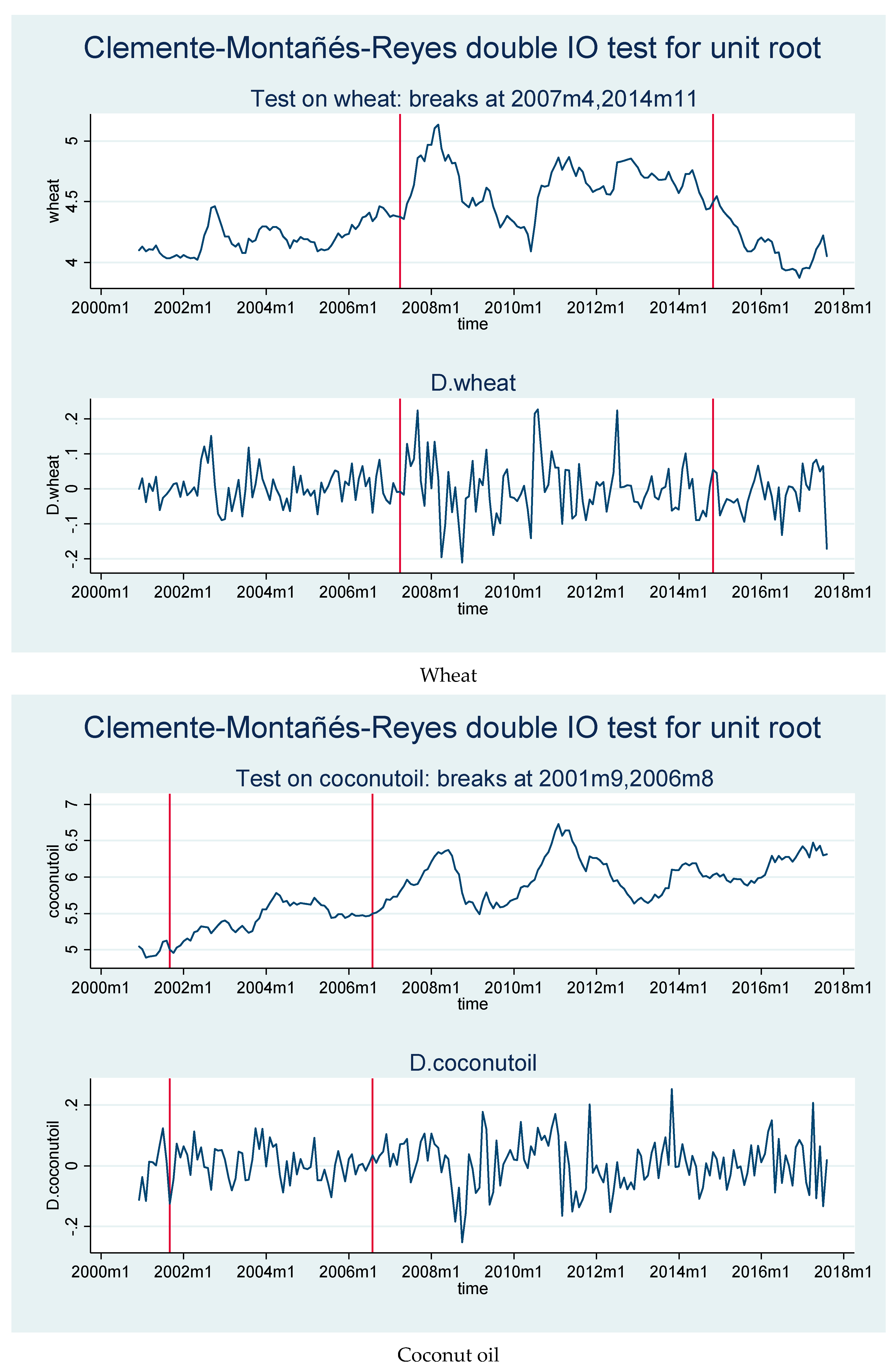
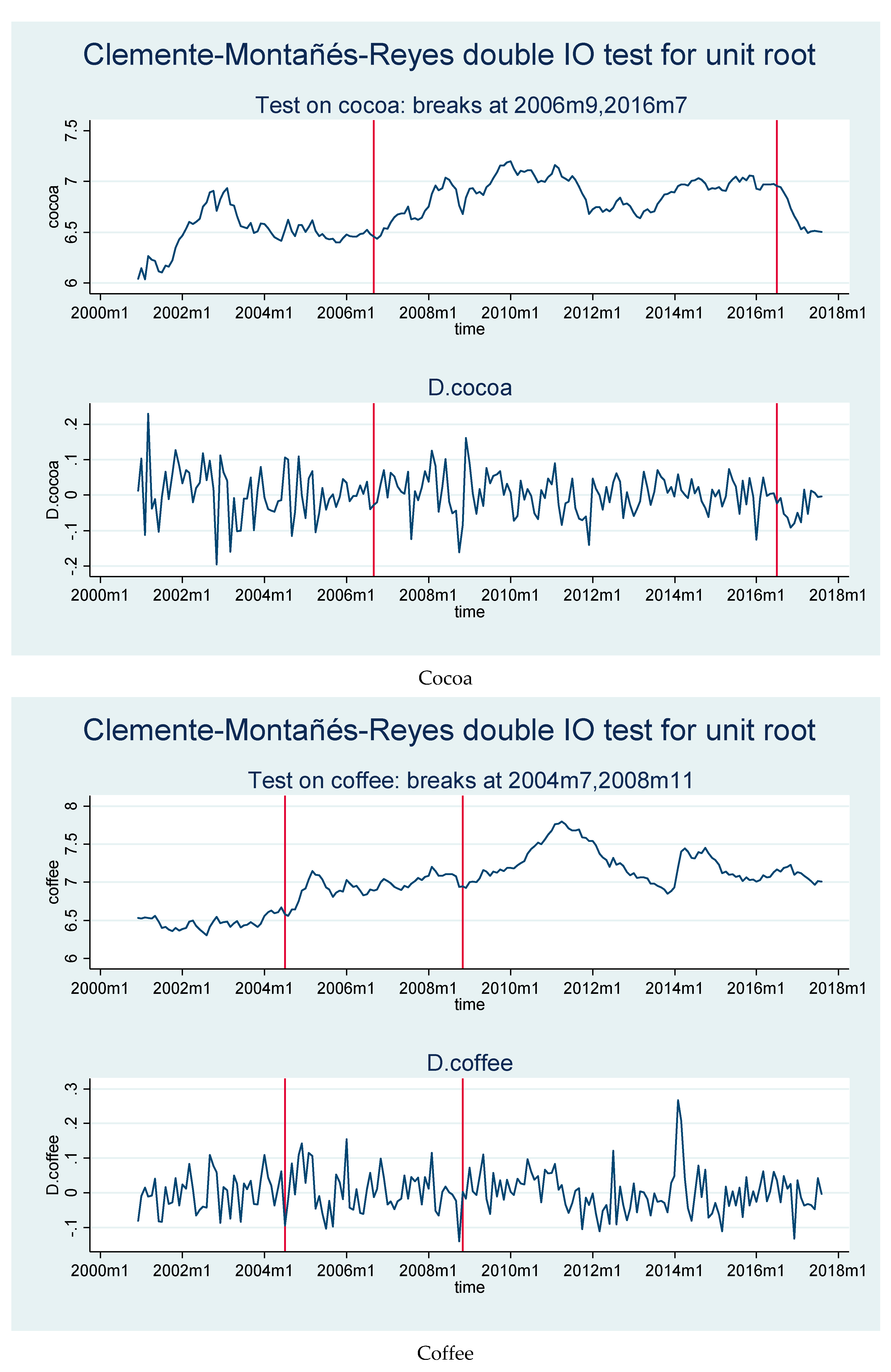
4. Data and Tests
5. Empirical Results
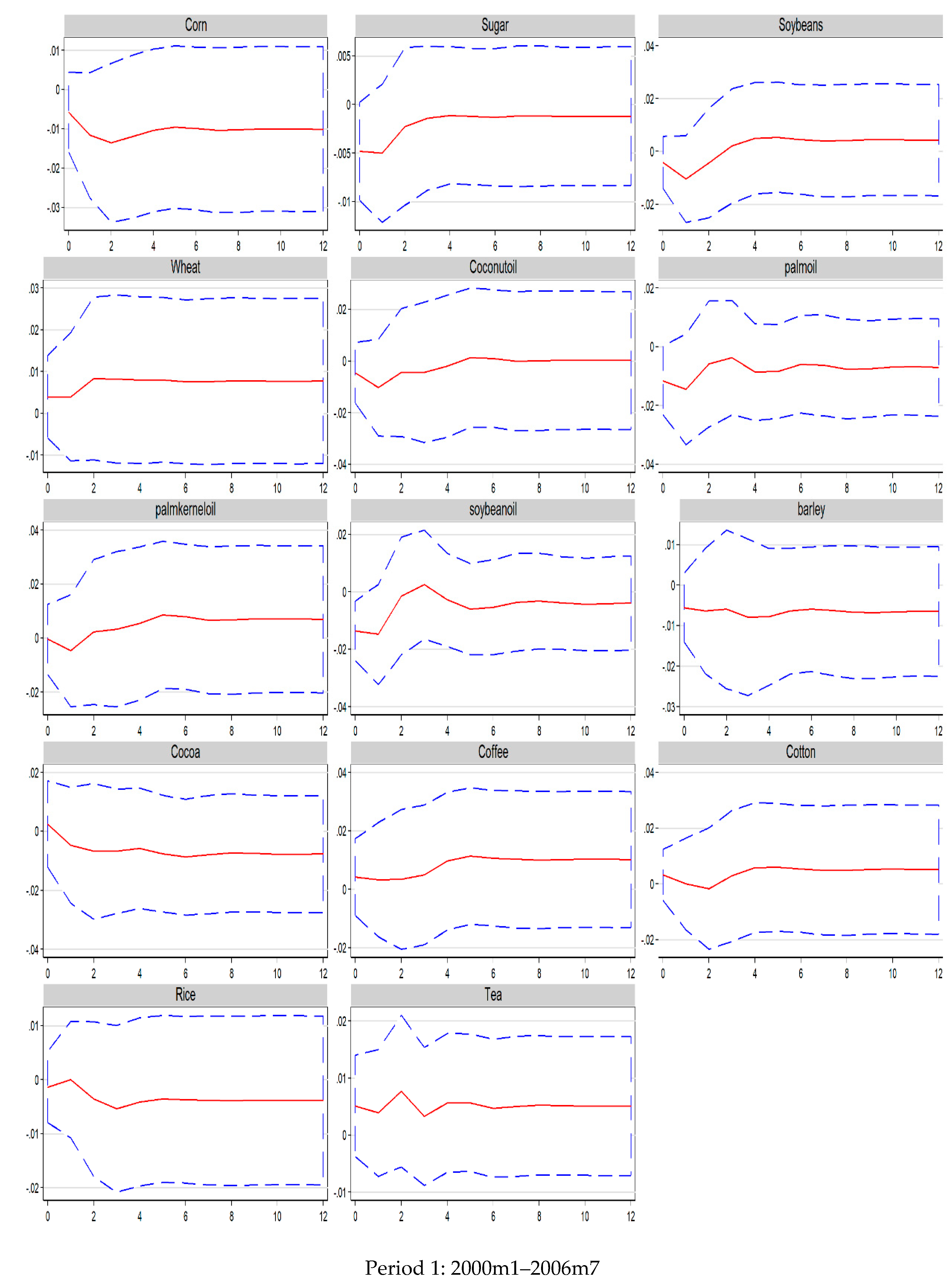
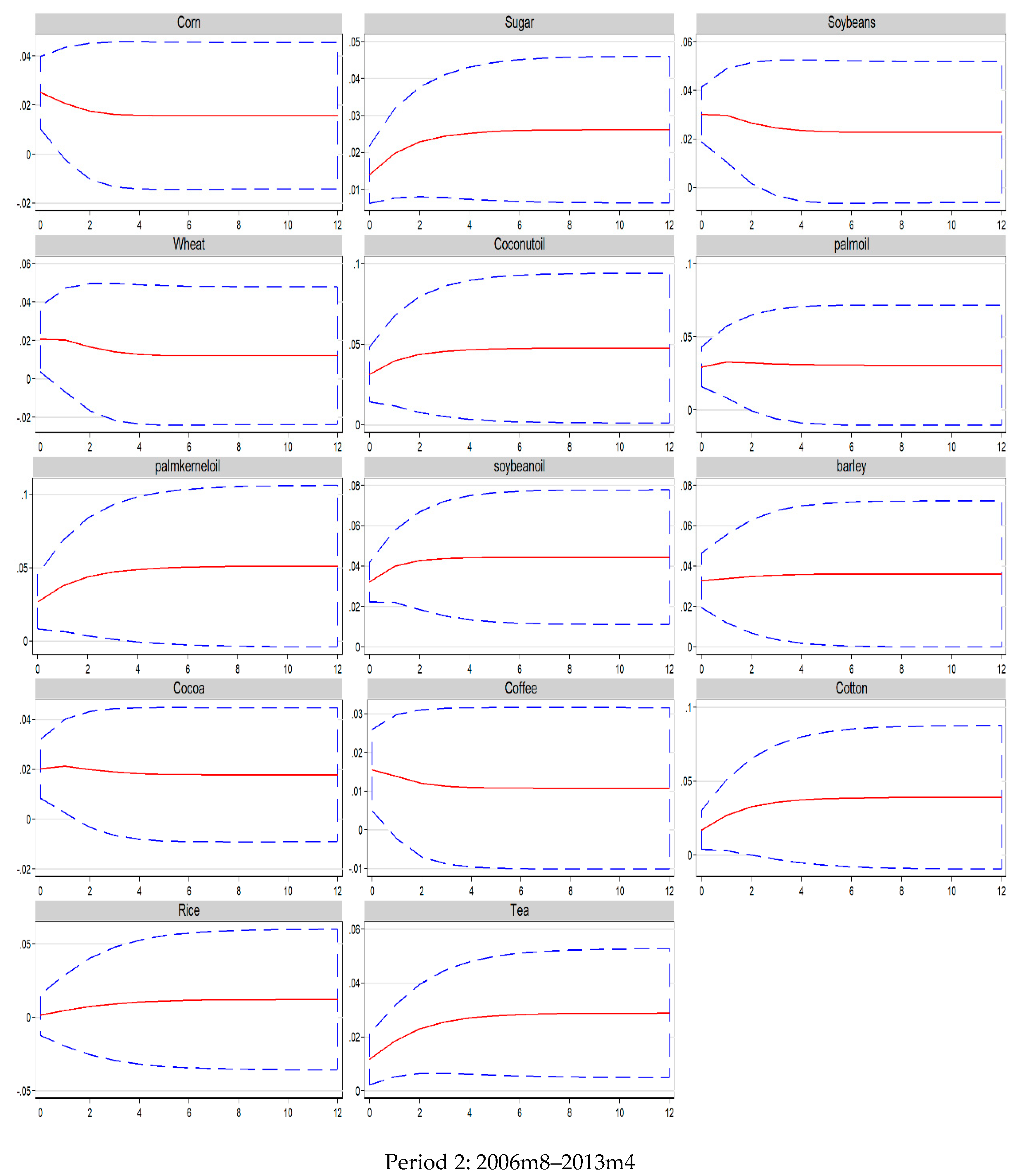
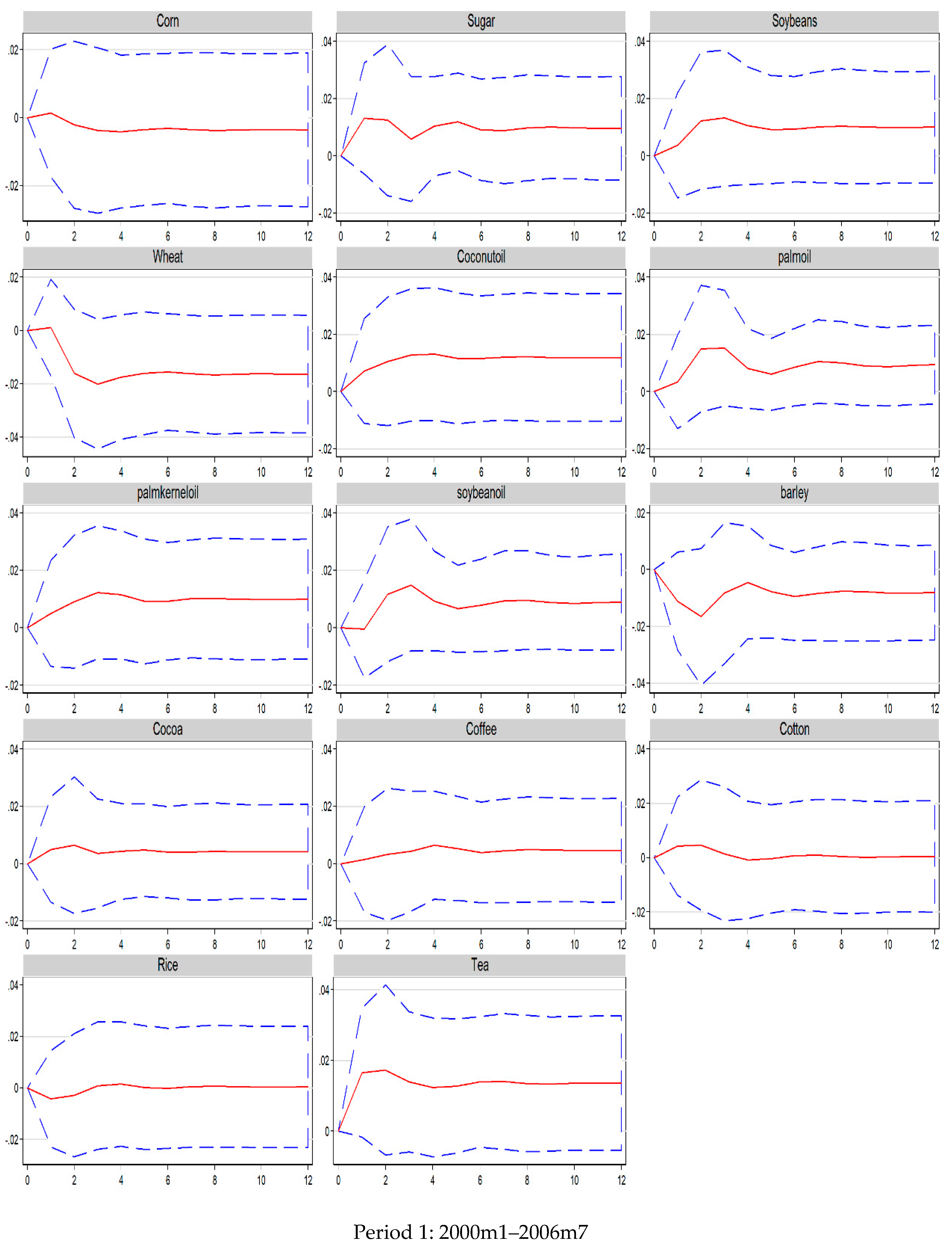
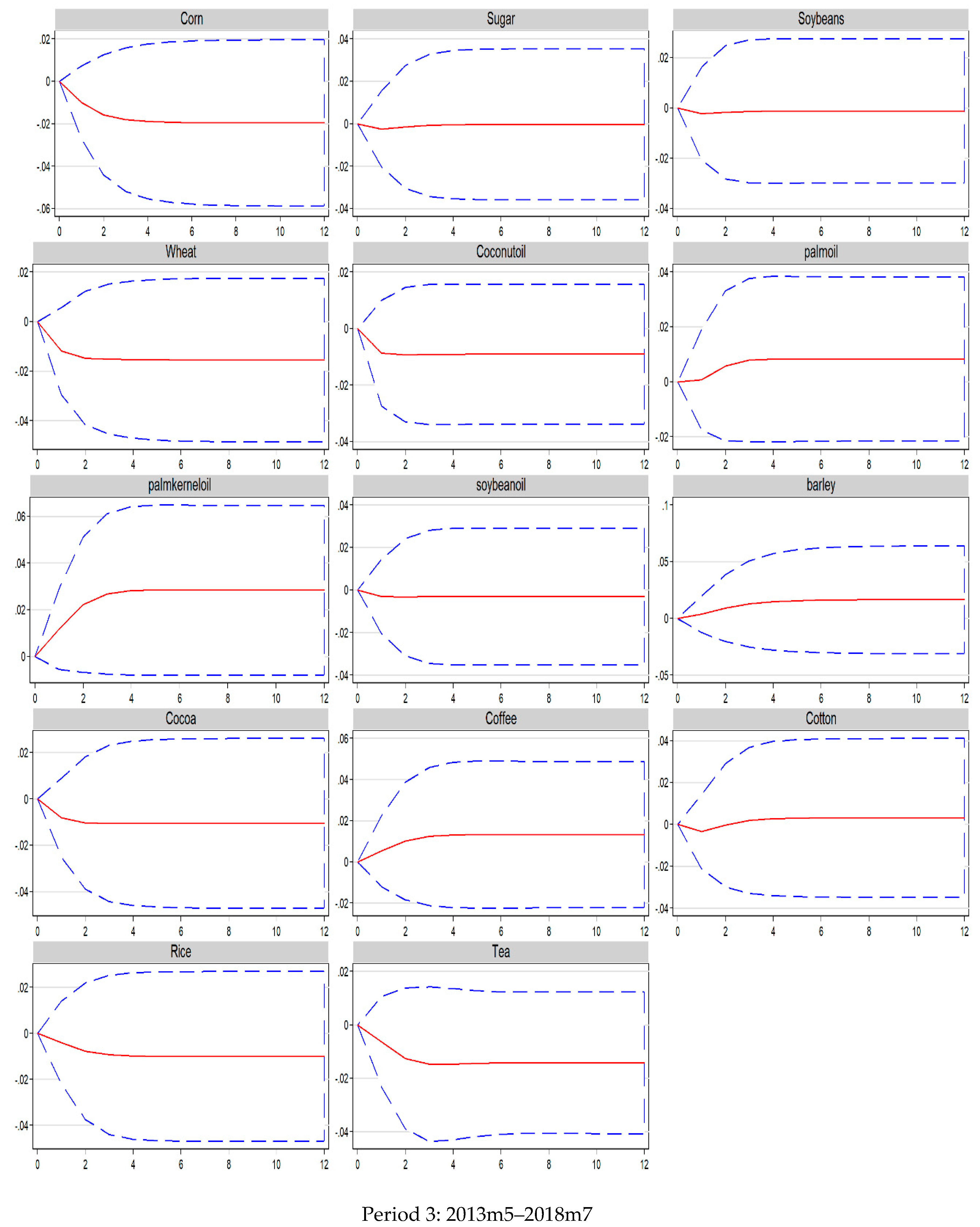
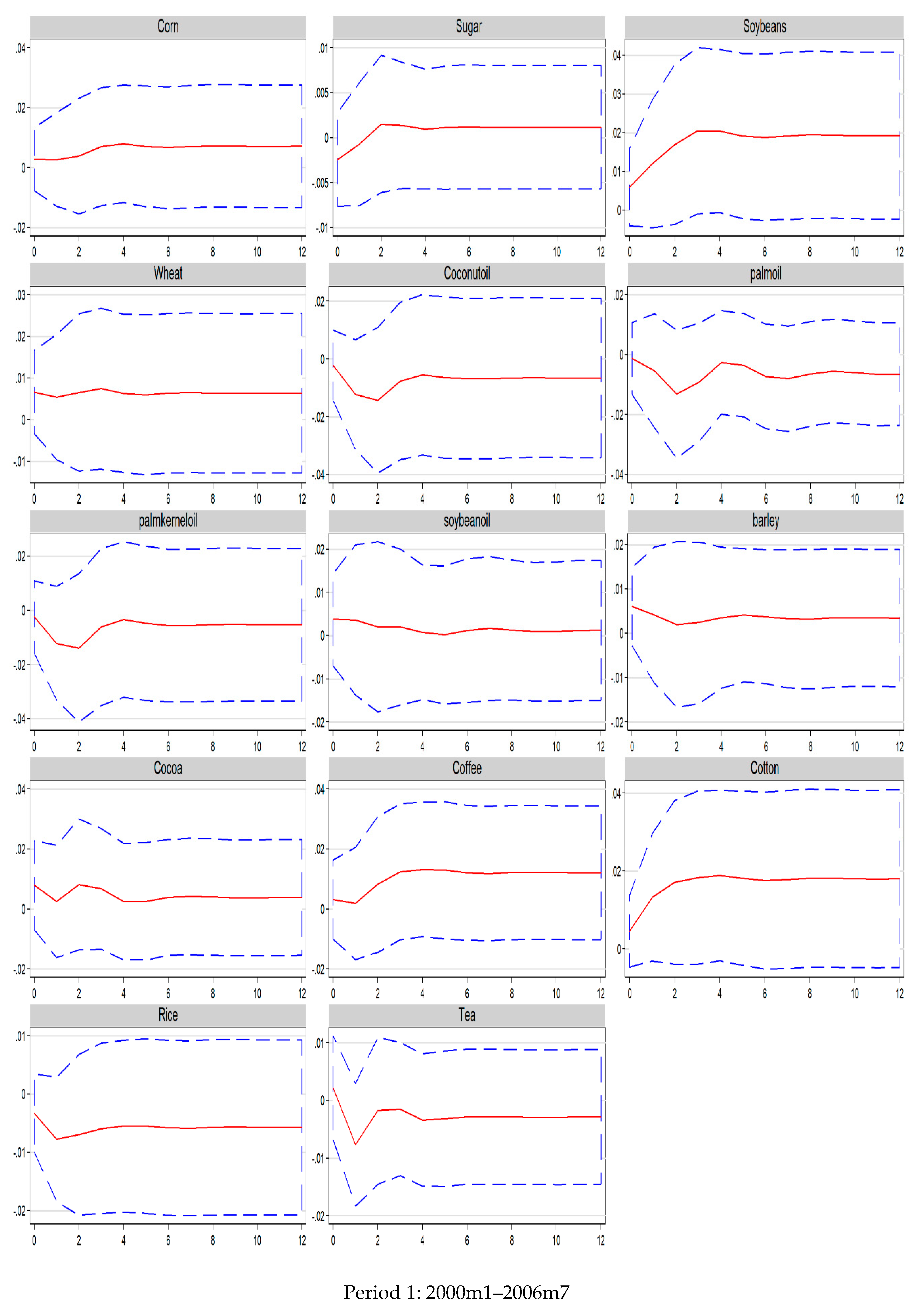
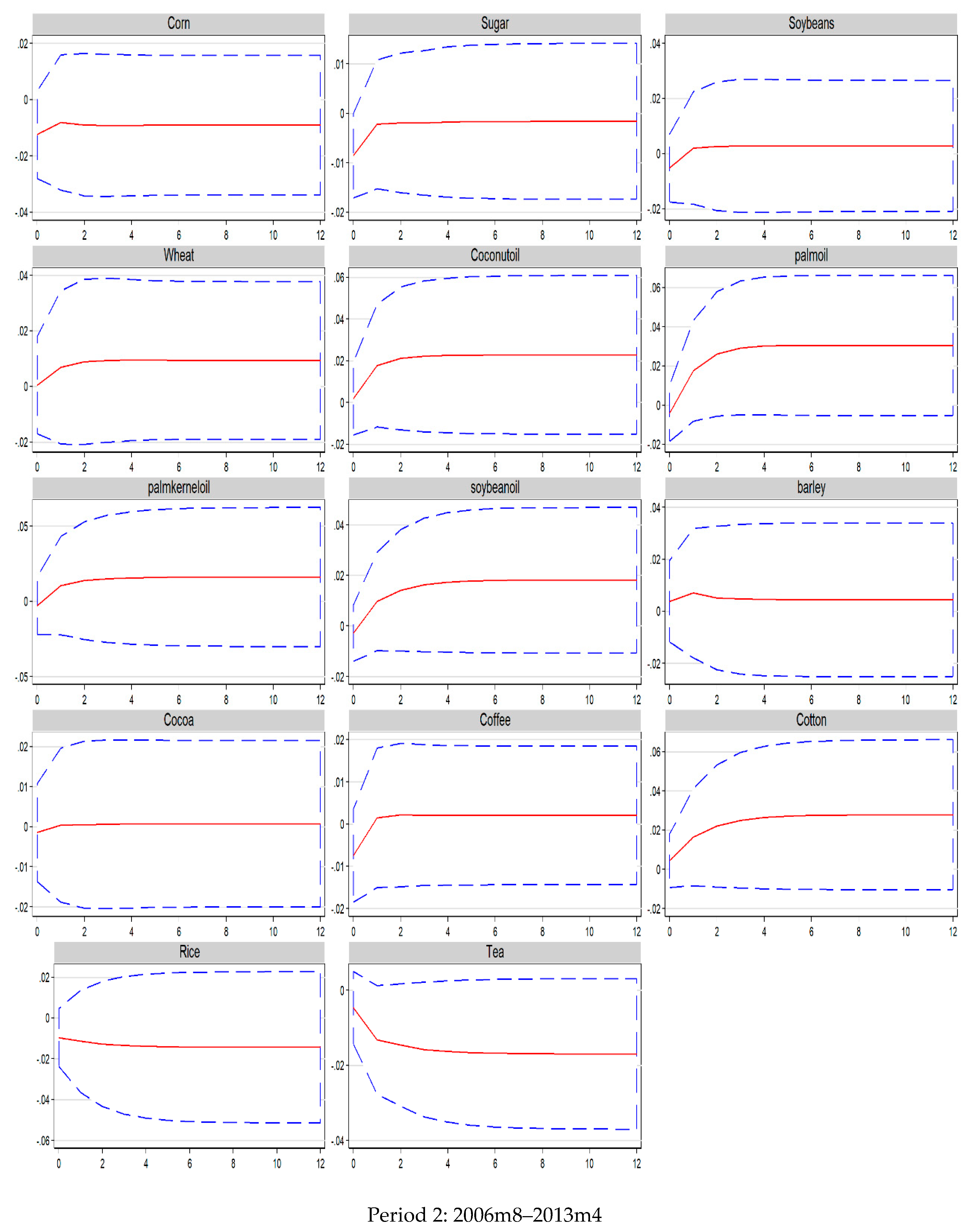
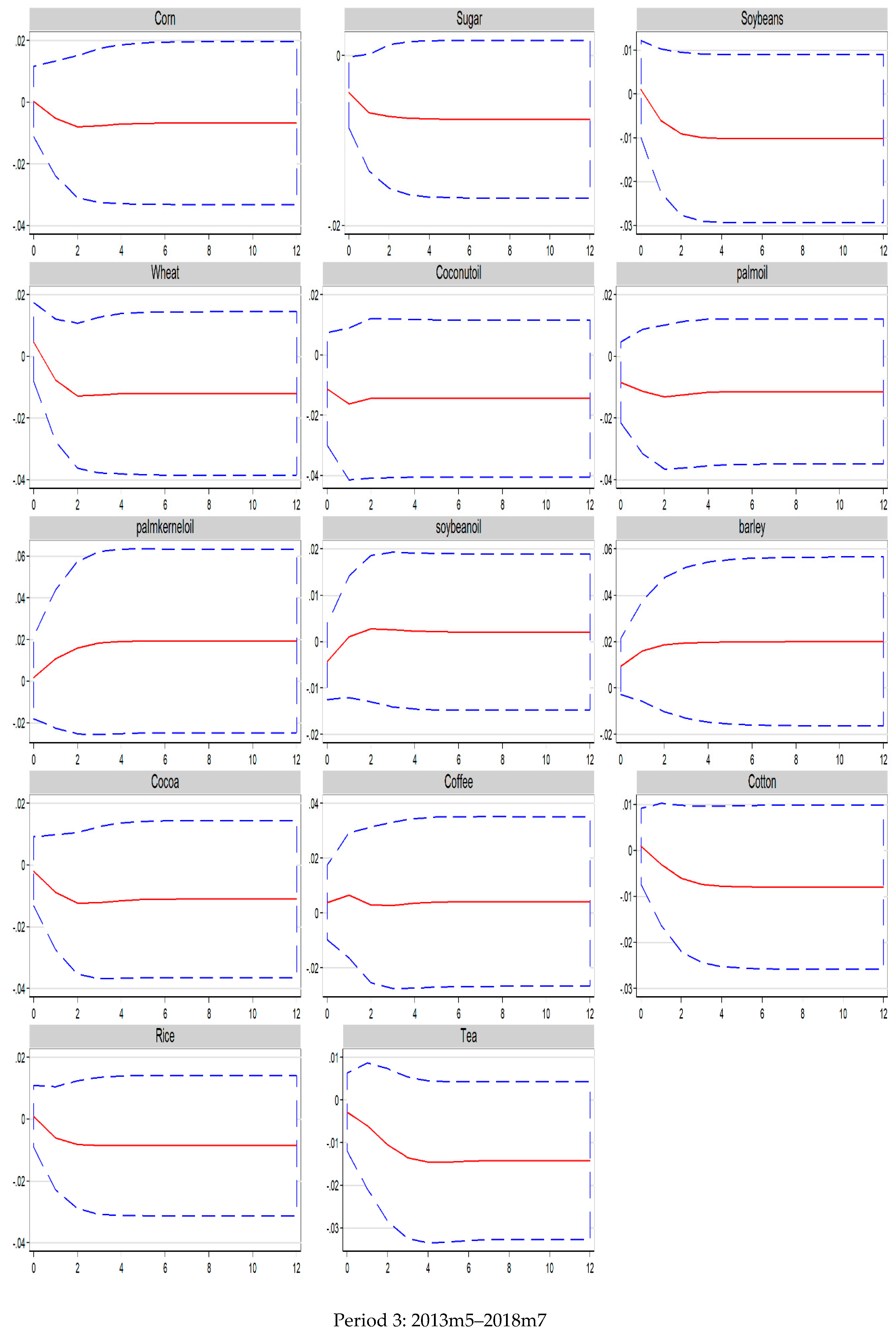
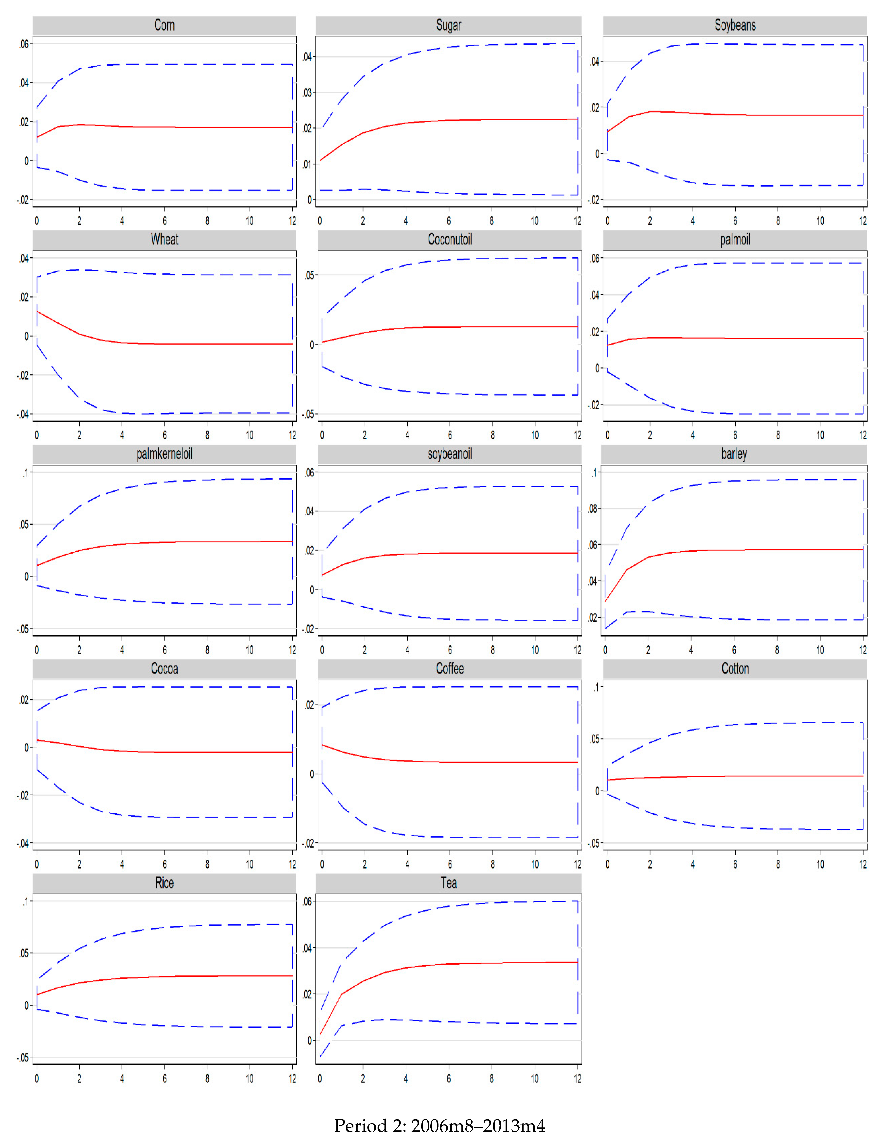
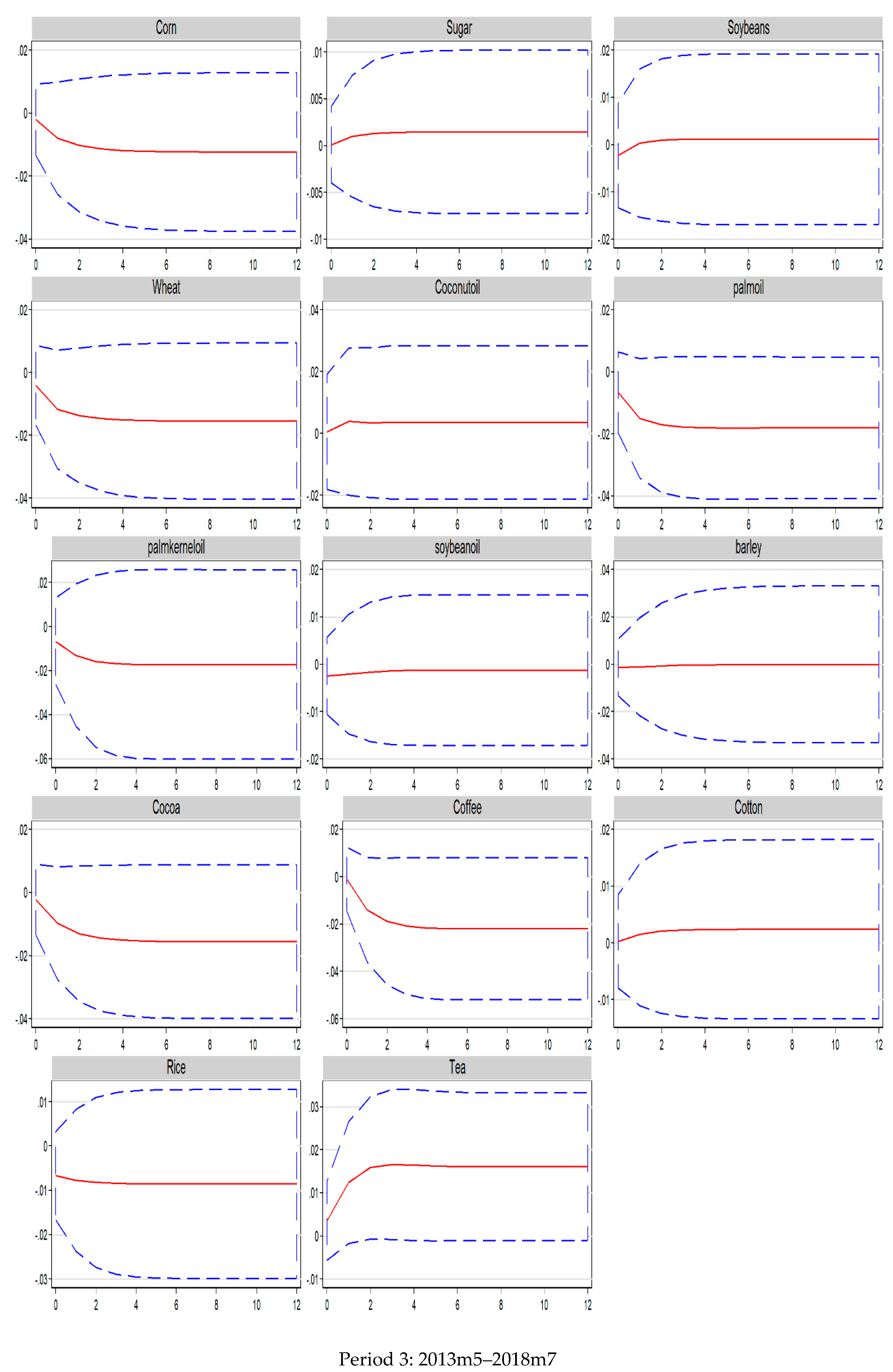
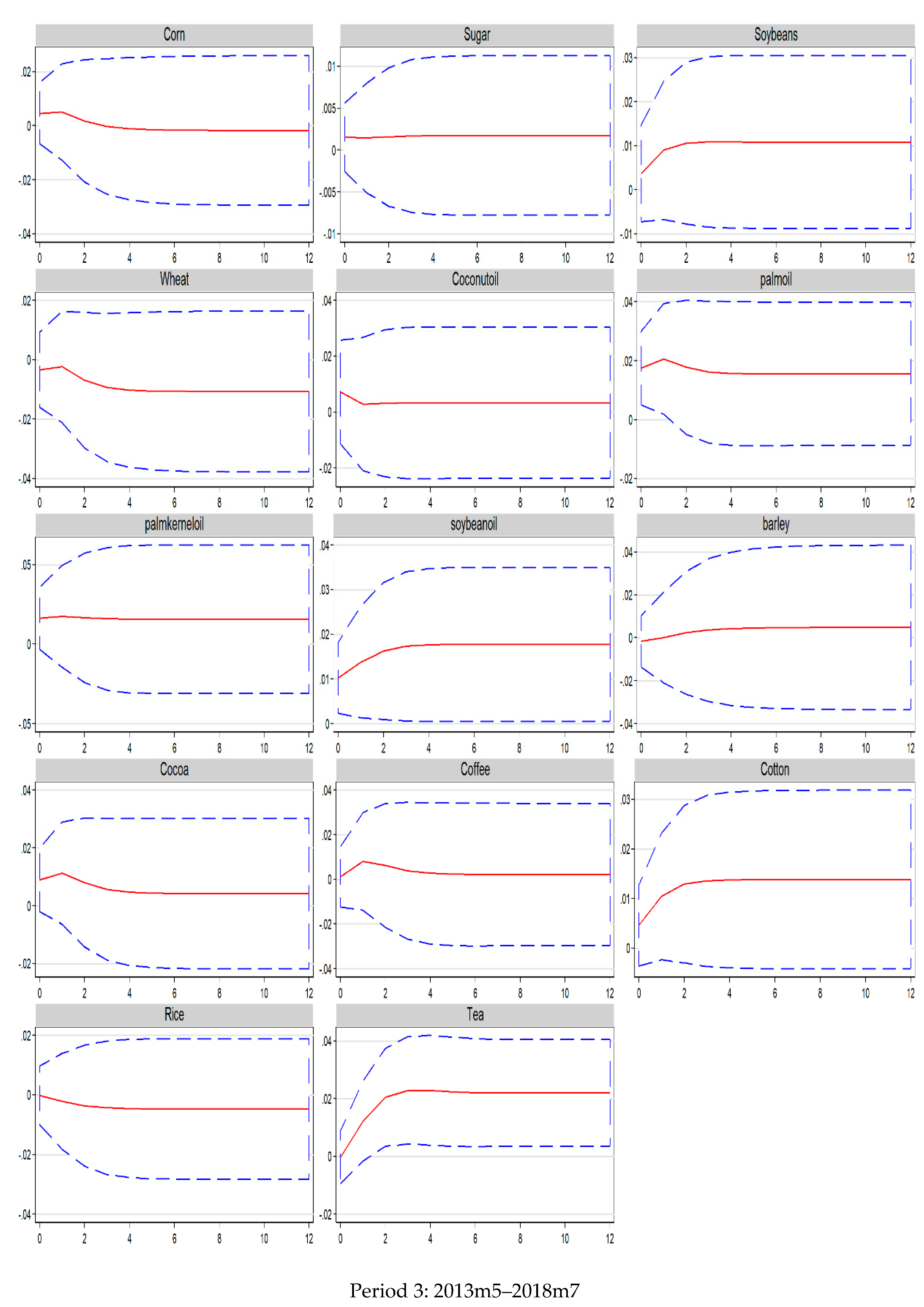
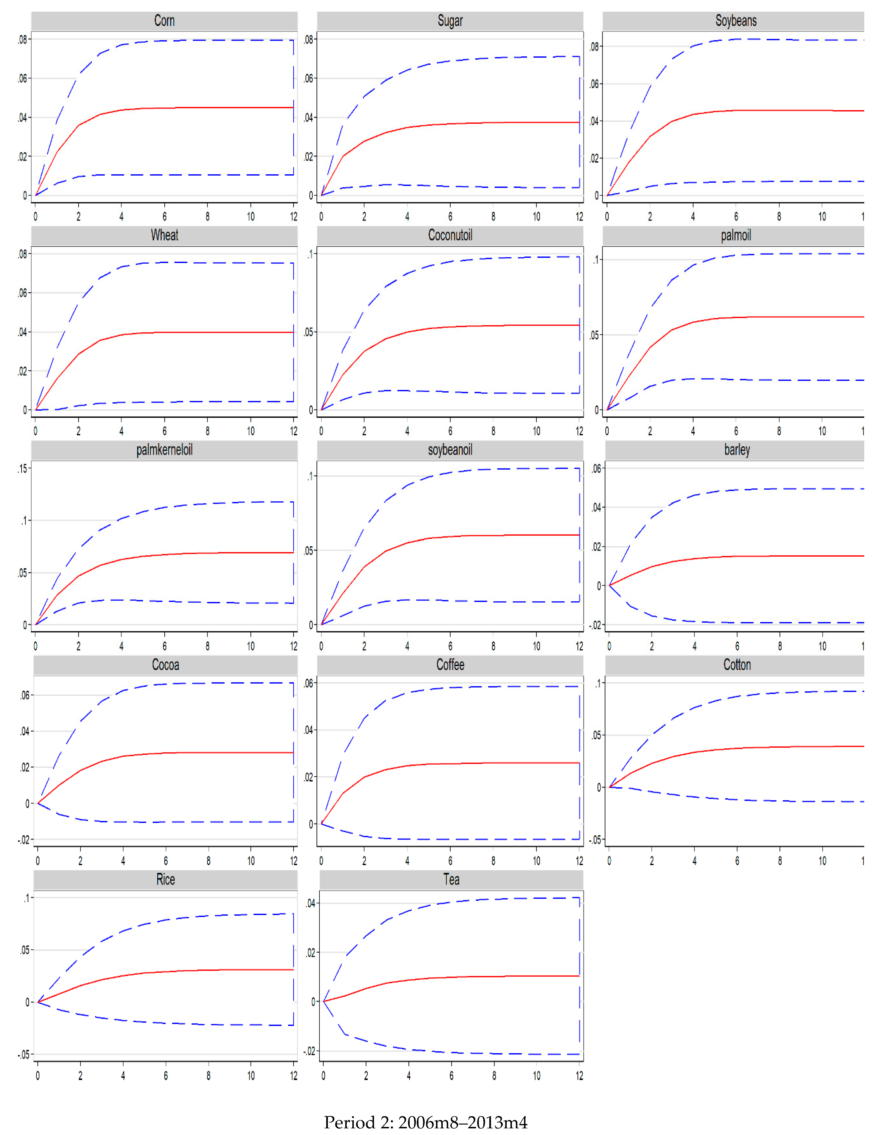
5.1. Responses of Agricultural Commodity Prices to Oil Shocks
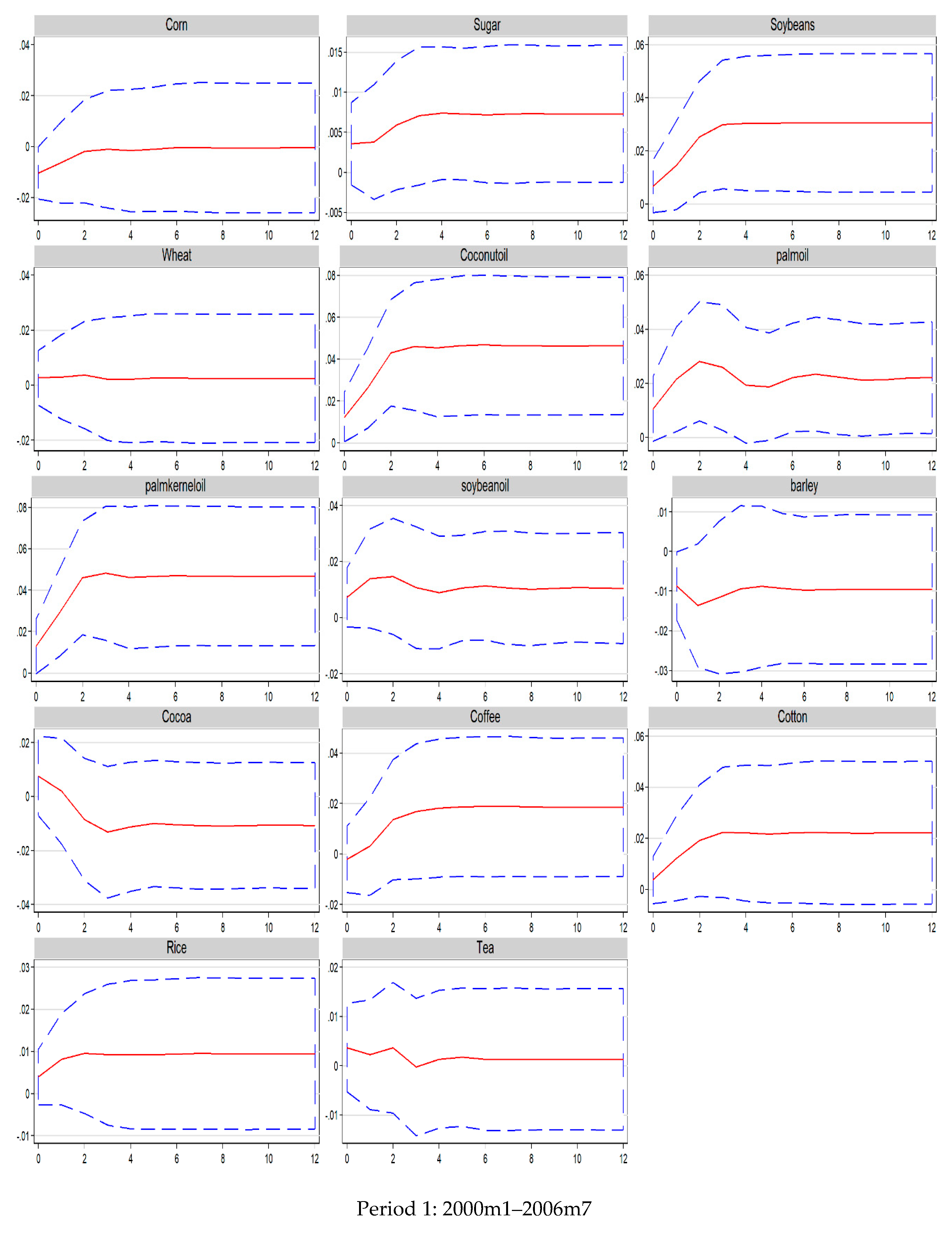
5.2. Responses of Crude Oil Price to Agricultural Shocks
5.3. Granger Causality Tests
5.4. Variance Decomposition
5.5. Discussion
6. Concluding Remarks
Author Contributions
Funding
Acknowledgments
Conflicts of Interest
References
- Guillouzouic-Le Corff, A. Did oil prices trigger an innovation burst in biofuels? Energy Econ. 2018, 75, 547–559. [Google Scholar] [CrossRef]
- Banse, M.; Van Meijl, H.; Tabeau, A.; Woltjer, G.; Hellmann, F.; Verburg, P.H. Impact of EU biofuel policies on world agricultural production and land use. Biomass Bioenergy 2010, 35, 2385–2390. [Google Scholar] [CrossRef]
- Renzaho, A.M.N.; Kamara, J.K.; Toole, M. Biofuel production and its impact on food security in low and middle income countries: Implications for the post-2015 sustainable development goals. Renew. Sustain. Energy Rev. 2017, 78, 503–516. [Google Scholar] [CrossRef]
- Kgathi, D.L.; Mfundisi, K.B.; Mmopelwa, G.; Mosepele, K. Potential impacts of biofuel development on food security in Botswana: A contribution to energy policy. Energy Policy 2009, 43, 70–79. [Google Scholar] [CrossRef]
- Chakravorty, U.; Hubert, M.; Moreaux, M.; Nøstbakken, L. Long-Run Impact of Biofuels on Food Prices. Scand. J. Econ. 2017, 119, 733–767. [Google Scholar] [CrossRef]
- Serra, T.; Zilberman, D. Biofuel-related price transmission literature: A review. Energy Econ. 2013, 37, 141–151. [Google Scholar] [CrossRef]
- Taghizadeh-hesary, F.; Rasoulinezhad, E.; Yoshino, N. Volatility Linkages between Energy and Food Prices; Asian Development Bank Institute: Chiyoda, Tokyo, 2018. [Google Scholar]
- Ciaian, P.; d’Artis, K. Interdependencies in the energy-bioenergy-food price systems: A cointegration analysis. Resour. Energy Econ. 2011, 33, 326–348. [Google Scholar] [CrossRef]
- Baumeister, C.; Kilian, L. Do oil price increases cause higher food prices? Econ. Policy 2014, 29, 691–747. [Google Scholar] [CrossRef]
- Dimitriadis, D.; Katrakilidis, C. An empirical analysis of the dynamic interactions among ethanol, crude oil and corn prices in the US market. Ann. Oper. Res. 2018, 1–11. [Google Scholar] [CrossRef]
- Nazlioglu, S.; Soytas, U. Oil price, agricultural commodity prices, and the dollar: A panel cointegration and causality analysis. Energy Econ. 2012, 34, 1098–1104. [Google Scholar] [CrossRef]
- Nazlioglu, S. World oil and agricultural commodity prices: Evidence from nonlinear causality. Energy Policy 2011, 39, 2935–2943. [Google Scholar] [CrossRef]
- Avalos, F. Do oil prices drive food prices? The tale of a structural break. J. Int. Money Financ. 2014, 42, 253–271. [Google Scholar] [CrossRef]
- Chiu, F.P.; Hsu, C.S.; Ho, A.; Chen, C.C. Modeling the price relationships between crude oil, energy crops and biofuels. Energy 2016, 109, 845–857. [Google Scholar] [CrossRef]
- Jadidzadeh, A.; Serletis, A. The global crude oil market and biofuel agricultural commodity prices. J. Econ. Asymmetries 2018, 18, e00094. [Google Scholar] [CrossRef]
- Amaiquema, J.R.P.; Amaiquema, A.R.P. Consequences of Oil and Food Price Shocks on the Ecuadorian Economy. Int. J. Energy Econ. Policy 2017, 7, 146–151. [Google Scholar]
- Ahmadi, M.; Behmiri, N.B.; Manera, M. How is volatility in commodity markets linked to oil price shocks? Energy Econ. 2016, 59, 11–23. [Google Scholar] [CrossRef]
- Jawad, S.; Shahzad, H.; Hernandez, J.A.; Al-yahyaee, K.H.; Jammazi, R. Asymmetric risk spillovers between oil and agricultural commodities. Energy Policy 2018, 118, 182–198. [Google Scholar]
- Kilian, L. Oil Price Shocks: Causes and Consequences. Annu. Rev. Resour. Econ. 2014, 6, 133–154. [Google Scholar] [CrossRef]
- López Cabrera, B.; Schulz, F. Volatility linkages between energy and agricultural commodity prices. Energy Econ. 2016, 54, 190–203. [Google Scholar] [CrossRef]
- Kapusuzoglu, A.; Karacaer Ulusoy, M. The interactions between agricultural commodity and oil prices: An empirical analysis. Agric. Econ. 2016, 61, 410–421. [Google Scholar] [CrossRef]
- Fernandez-Perez, A.; Frijns, B.; Tourani-Rad, A. Contemporaneous interactions among fuel, biofuel and agricultural commodities. Energy Econ. 2016, 58, 1–10. [Google Scholar] [CrossRef]
- Wang, Y.; Wu, C.; Yang, L. Oil price shocks and agricultural commodity prices. Energy Econ. 2014, 44, 22–35. [Google Scholar] [CrossRef]
- Fowowe, B. Do oil prices drive agricultural commodity prices? Evidence from South Africa. Energy 2016, 104, 149–157. [Google Scholar] [CrossRef]
- Nazlioglu, S.; Soytas, U. World oil prices and agricultural commodity prices: Evidence from an emerging market. Energy Econ. 2011, 33, 488–496. [Google Scholar] [CrossRef]
- Zhang, Z.; Lohr, L.; Escalante, C.; Wetzstein, M. Food versus fuel: What do prices tell us? Energy Policy 2010, 38, 445–451. [Google Scholar] [CrossRef]
- Rosa, F.; Vasciaveo, M. Agri-commodity price dynamics: The relationship between oil and agricultural market. In Proceedings of the International Association of Agricultural Economists (IAAE) Triennial Conference, Foz do Iguaçu, Brazil, 18–24 August 2012; pp. 18–24. [Google Scholar]
- Diks, C.; Panchenko, V. A new statistic and practical guidelines for nonparametric Granger causality testing. J. Econ. Dyn. Control 2006, 30, 1647–1669. [Google Scholar] [CrossRef]
- Chang, C.-L.; Li, Y.; McAleer, M. Volatility spillovers between energy and agricultural markets: A critical appraisal of theory and practice. Energies 2018, 11, 1595. [Google Scholar] [CrossRef]
- Chang, C.; Mcaleer, M.; Wang, Y. Modelling volatility spillovers for bio-ethanol, sugarcane and corn spot and futures prices. Renew. Sustain. Energy Rev. 2018, 81, 1002–1018. [Google Scholar] [CrossRef]
- Nazlioglu, S.; Erdem, C.; Soytas, U. Volatility spillover between oil and agricultural commodity markets. Energy Econ. 2013, 36, 658–665. [Google Scholar] [CrossRef]
- Hafner, C.M.; Herwartz, H. A Lagrange multiplier test for causality in variance. Econ. Lett. 2006, 93, 137–141. [Google Scholar] [CrossRef]
- Chang, C.-L.; McAleer, M. A simple test for causality in volatility. Econometrics 2017, 5, 15. [Google Scholar] [CrossRef]
- Adam, P.; Rosnawintang, R.; Tondi, L. The causal relationship between crude oil price, exchange rate and rice price. Int. J. Energy Econ. Policy 2018, 8, 90–94. [Google Scholar]
- Chen, P.-Y.; Chang, C.-L.; Chen, C.-C.; McAleer, M. Modelling the effects of oil prices on global fertilizer prices and volatility. J. Risk Financ. Manag. 2012, 5, 78–114. [Google Scholar] [CrossRef]
- Lucotte, Y. Co-movements between crude oil and food prices: A post-commodity boom perspective. Econ. Lett. 2016, 147, 142–147. [Google Scholar] [CrossRef]
- Paris, A. On the link between oil and agricultural commodity prices: Do biofuels matter? Int. Econ. 2018, 155, 48–60. [Google Scholar] [CrossRef]
- Choi, I. Testing linearity in cointegrating smooth transition regressions. Econ. J. 2004, 7, 341–365. [Google Scholar] [CrossRef]
- Kilian, L. Not all oil price shocks are alike: Disentangling demand and supply shocks in the crude oil market. Am. Econ. Rev. 2009, 99, 1053–1069. [Google Scholar] [CrossRef]
- Ramcharran, H. Oil production responses to price changes: An empirical application of the competitive model to OPEC and non-OPEC countries. Energy Econ. 2002, 24, 97–106. [Google Scholar] [CrossRef]
- Bointner, R.; Pezzutto, S.; Sparber, W. Scenarios of public energy research and development expenditures: Financing energy innovation in Europe. WIREs Energy Environ. 2006, 5, 470–488. [Google Scholar] [CrossRef]
- Bointner, R.; Pezzutto, S.; Grilli, G.; Sparber, W. Financing innovations for the renewable energy transition in Europe. Energies 2016, 9, 990. [Google Scholar] [CrossRef]
- Qiu, C.; Colson, G.; Escalante, C.; Wetzstein, M. Considering macroeconomic indicators in the food before fuel nexus. Energy Econ. 2012, 34, 2021–2028. [Google Scholar] [CrossRef]
- Mcphail, L.L. Assessing the impact of US ethanol on fossil fuel markets: A structural VAR approach. Energy Econ. 2011, 33, 1177–1185. [Google Scholar] [CrossRef]
- Perron, P.; Vogelsang, T.J. Nonstationarity and level shifts with an application to purchasing power parity. J. Bus. Econ. Stat. 1992, 10, 301–320. [Google Scholar]
- Clemente, J.; Montañés, A.; Reyes, M. Testing for a unit root in variables with a double change in the mean. Econ. Lett. 1998, 59, 175–182. [Google Scholar] [CrossRef]
- Kilian, L. Measuring Global Economic Activity: Reply; University of Michigan: Ann Arbor, MI, USA, 2018; pp. 1–5. [Google Scholar]
- Dickey, D.A.; Fuller, W.A. Distribution of the estimators for autoregressive time series with a unit root. J. Am. Stat. Assoc. 1979, 74, 427–431. [Google Scholar]
- Zivot, E.; Andrews, D.W.K. Further evidence on the great crash, the oil-price shock, and the unit-root hypothesis. J. Bus. Econ. Stat. 2002, 20, 25–44. [Google Scholar] [CrossRef]
- Gregory, A.W.; Hansen, B.E. Residual-based tests for cointegration in models with regime shifts. J. Econ. 1996, 70, 99–126. [Google Scholar] [CrossRef]
- Zhang, C.; Qu, X. The effect of global oil price shocks on China’s agricultural commodities. Energy Econ. 2015, 51, 354–364. [Google Scholar] [CrossRef]
- Gomiero, T. Are biofuels an effective and viable energy strategy for industrialized societies? A reasoned overview of potentials and limits. Sustainability 2015, 7, 8491–8521. [Google Scholar] [CrossRef]
- Gasparatos, A.; Stromberg, P.; Takeuchi, K. Sustainability impacts of first-generation biofuels. Anim. Front. 2013, 3, 12–26. [Google Scholar] [CrossRef]


| January 2000–July 2006 | ||||||
| Variable | Mean | SD | Max | Min | Skewness | Kurtosis |
| Brent | 2.715 | 0.321 | 3.401 | 2.156 | 0.591 | 2.331 |
| Corn | 3.791 | 0.098 | 4.072 | 3.581 | 0.605 | 3.407 |
| Sugar | 5.586 | 0.067 | 5.714 | 5.470 | 0.127 | 1.945 |
| Soybeans | 4.683 | 0.156 | 5.203 | 4.448 | 0.970 | 4.192 |
| Wheat | 4.157 | 0.124 | 4.460 | 3.925 | 0.290 | 2.668 |
| Coconut oil | 5.369 | 0.240 | 5.779 | 4.893 | −0.256 | 2.048 |
| Palm oil | 5.146 | 0.182 | 5.490 | 4.689 | −0.688 | 3.169 |
| Palm kernel oil | 5.356 | 0.252 | 5.767 | 4.836 | −0.348 | 1.997 |
| Soybean oil | 5.350 | 0.214 | 5.718 | 4.921 | −0.373 | 2.023 |
| Barley | 3.764 | 0.121 | 4.011 | 3.548 | 0.300 | 2.205 |
| Cocoa | 6.439 | 0.238 | 6.931 | 6.029 | −0.144 | 2.376 |
| Coffee | 6.654 | 0.234 | 7.147 | 6.303 | 0.475 | 1.875 |
| Cotton | 6.296 | 0.160 | 6.628 | 5.941 | 0.041 | 2.408 |
| Rice | 4.582 | 0.159 | 4.853 | 4.335 | 0.378 | 1.739 |
| Tea | 6.605 | 0.102 | 6.885 | 6.437 | 1.010 | 3.155 |
| August 2006–April 2013 | ||||||
| Variable | Mean | SD | Max | Min | Skewness | Kurtosis |
| Brent | 3.472 | 0.263 | 3.920 | 2.785 | −0.600 | 2.788 |
| Corn | 4.380 | 0.259 | 4.788 | 3.853 | 0.036 | 1.552 |
| Sugar | 5.291 | 0.245 | 5.708 | 4.975 | 0.396 | 1.576 |
| Soybeans | 5.172 | 0.200 | 5.502 | 4.652 | −0.636 | 2.827 |
| Wheat | 4.613 | 0.220 | 5.134 | 4.091 | 0.043 | 2.300 |
| Coconut oil | 5.966 | 0.322 | 6.731 | 5.490 | 0.497 | 2.232 |
| Palm oil | 5.775 | 0.243 | 6.178 | 5.240 | −0.302 | 2.279 |
| Palm kernel oil | 5.932 | 0.342 | 6.748 | 5.317 | 0.273 | 2.348 |
| Soybean oil | 5.967 | 0.218 | 6.367 | 5.499 | −0.187 | 2.085 |
| Barley | 4.211 | 0.227 | 4.556 | 3.676 | −0.445 | 2.156 |
| Cocoa | 6.857 | 0.198 | 7.197 | 6.437 | −0.160 | 2.030 |
| Coffee | 7.226 | 0.257 | 7.797 | 6.891 | 0.782 | 2.423 |
| Cotton | 6.536 | 0.318 | 7.534 | 6.087 | 1.380 | 4.666 |
| Rice | 5.229 | 0.237 | 5.856 | 4.794 | −0.163 | 3.040 |
| Tea | 6.881 | 0.145 | 7.094 | 6.567 | −0.705 | 2.247 |
| May 2013–July 2018 | ||||||
| Variable | Mean | SD | Max | Min | Skewness | Kurtosis |
| Brent | 3.103 | 0.369 | 3.673 | 2.367 | 0.298 | 1.906 |
| Corn | 4.097 | 0.175 | 4.661 | 3.897 | 1.534 | 5.216 |
| Sugar | 4.893 | 0.097 | 5.060 | 4.761 | 0.618 | 1.879 |
| Soybeans | 5.011 | 0.137 | 5.331 | 4.825 | 0.804 | 2.482 |
| Wheat | 4.294 | 0.266 | 4.757 | 3.874 | 0.362 | 1.827 |
| Coconut oil | 6.081 | 0.197 | 6.475 | 5.684 | −0.126 | 2.291 |
| Palm oil | 5.444 | 0.188 | 5.816 | 5.092 | 0.344 | 2.226 |
| Palm kernel oil | 5.920 | 0.196 | 6.377 | 5.556 | 0.230 | 2.165 |
| Soybean oil | 5.601 | 0.158 | 5.943 | 5.364 | 0.690 | 2.229 |
| Barley | 3.748 | 0.252 | 4.410 | 3.421 | 0.813 | 3.095 |
| Cocoa | 6.819 | 0.190 | 7.059 | 6.457 | −0.581 | 1.872 |
| Coffee | 7.090 | 0.164 | 7.452 | 6.850 | 0.634 | 2.506 |
| Cotton | 6.413 | 0.117 | 6.615 | 6.214 | 0.072 | 1.674 |
| Rice | 4.953 | 0.098 | 5.263 | 4.819 | 0.956 | 4.001 |
| Tea | 6.881 | 0.073 | 7.004 | 6.685 | −0.472 | 2.993 |
| Levels | |||||
| ADF | ZA | CMR | |||
| Level | T-Stat | Break in | Mint t | Break in | |
| Oil production | −1.415 | −3.654; −2.853; −3.746 | Intercept (2008m8); Trend (2012m8); Both Intercept and Trend (2003m1) | −5.269 | 2003m6; 2015m1 |
| Kilian’s index | −2.419 | −3.939; −3.598; −4.649 | Intercept (2010m6); Trend (2004m8); Both Intercept and Trend (2008m9) | −4.336 | 2003m1; 2010m4 |
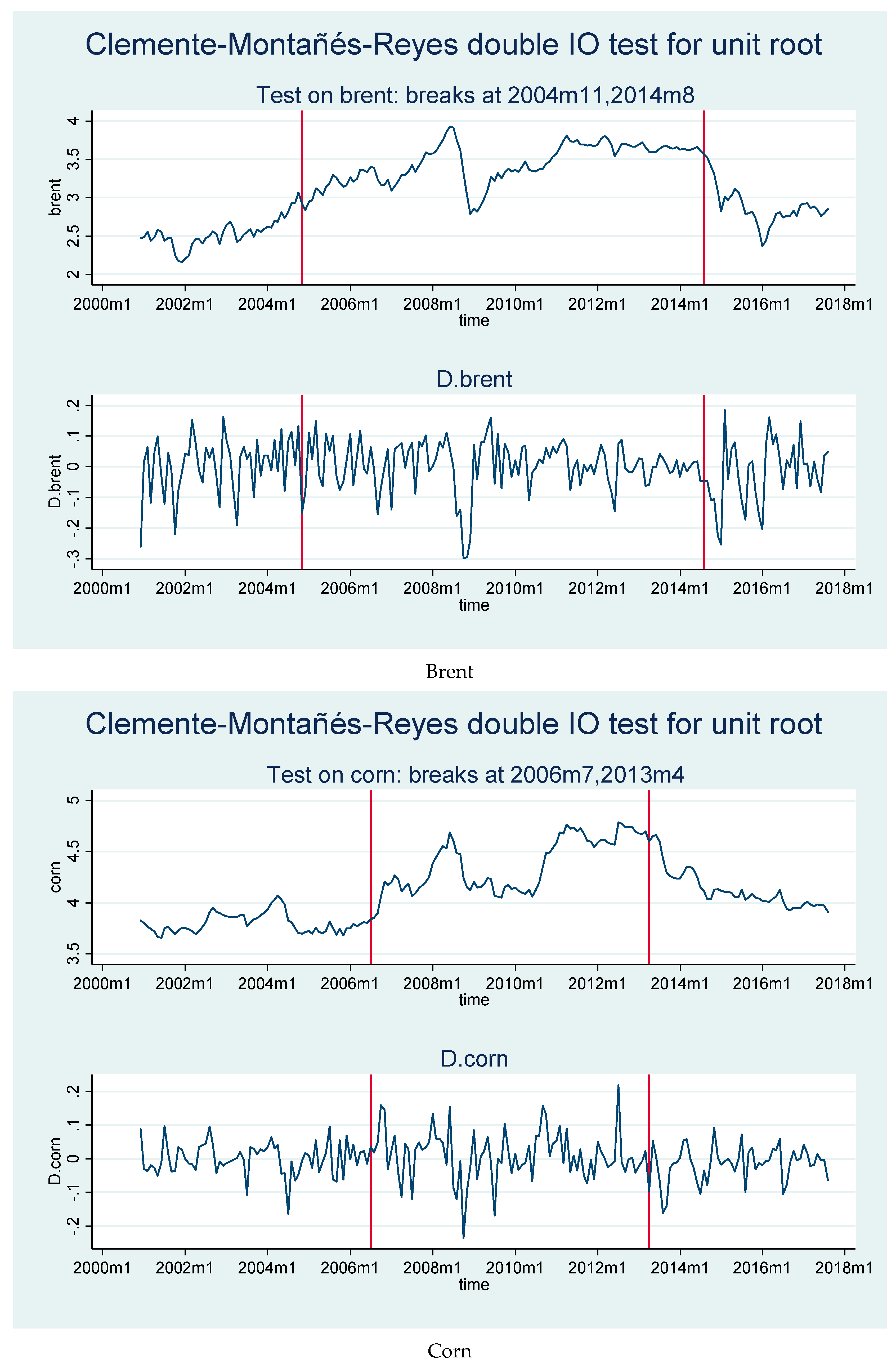
| Brent | −2.028 | −4.384; −3.339; −3.895 | Intercept (2014m7); Trend (2011m3); Both Intercept and Trend (2014m10) | −4.31 | 2004m11; 2014m8 |
| Corn | −1.964 | −3.957; −3.785; −4.702 | Intercept (2013m7); Trend (2012m2); Both Intercept and Trend (2010m7) | −4.366 | 2006m7; 2013m4 |
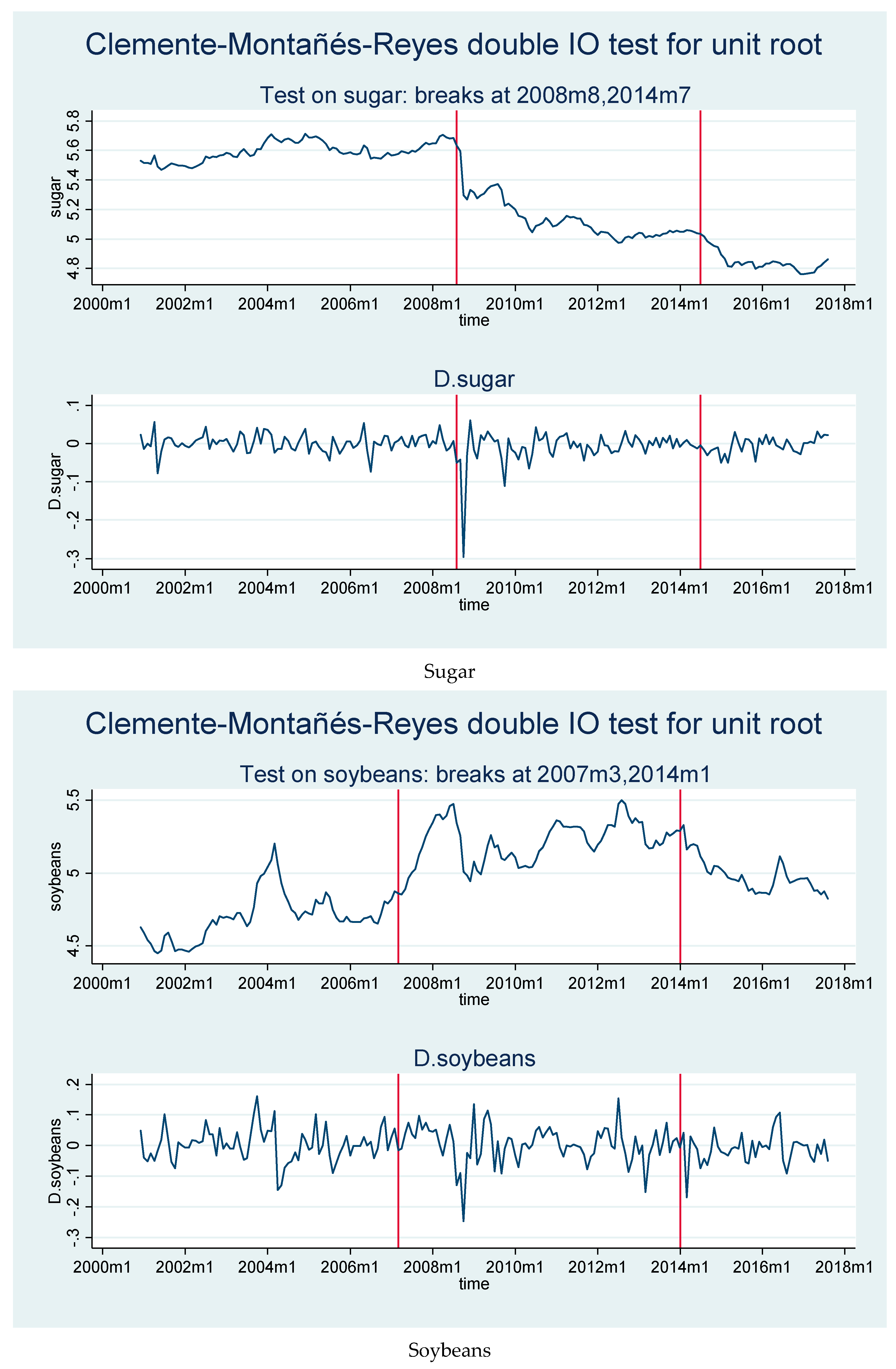
| Sugar | −0.577 | −4.162; −3.398; −6.192 *** | Intercept (2008m10); Trend (2004m1); Both Intercept and Trend (2008m10) | −6.159 ** | 2008m8; 2014m7 |
| Soybeans | −2.211 | −4.352; −4.259 *; −4.569 | Intercept (2014m3); Trend (2012m3); Both Intercept and Trend (2007m5) | −4.547 | 2007m3; 2014m1 |
| Wheat | −2.373 | −4.272; −3.54; −4.045 | Intercept (2014m6); Trend (2011m5); Both Intercept and Trend (2010m7) | −5.041 | 2007m4; 2014m11 |
| Coconut oil | −1.973 | −4.081; −3.953; −4.309 | Intercept (2012m2); Trend (2010m12); Both Intercept and Trend (2012m2) | −4.479 | 2001m9; 2006m8 |
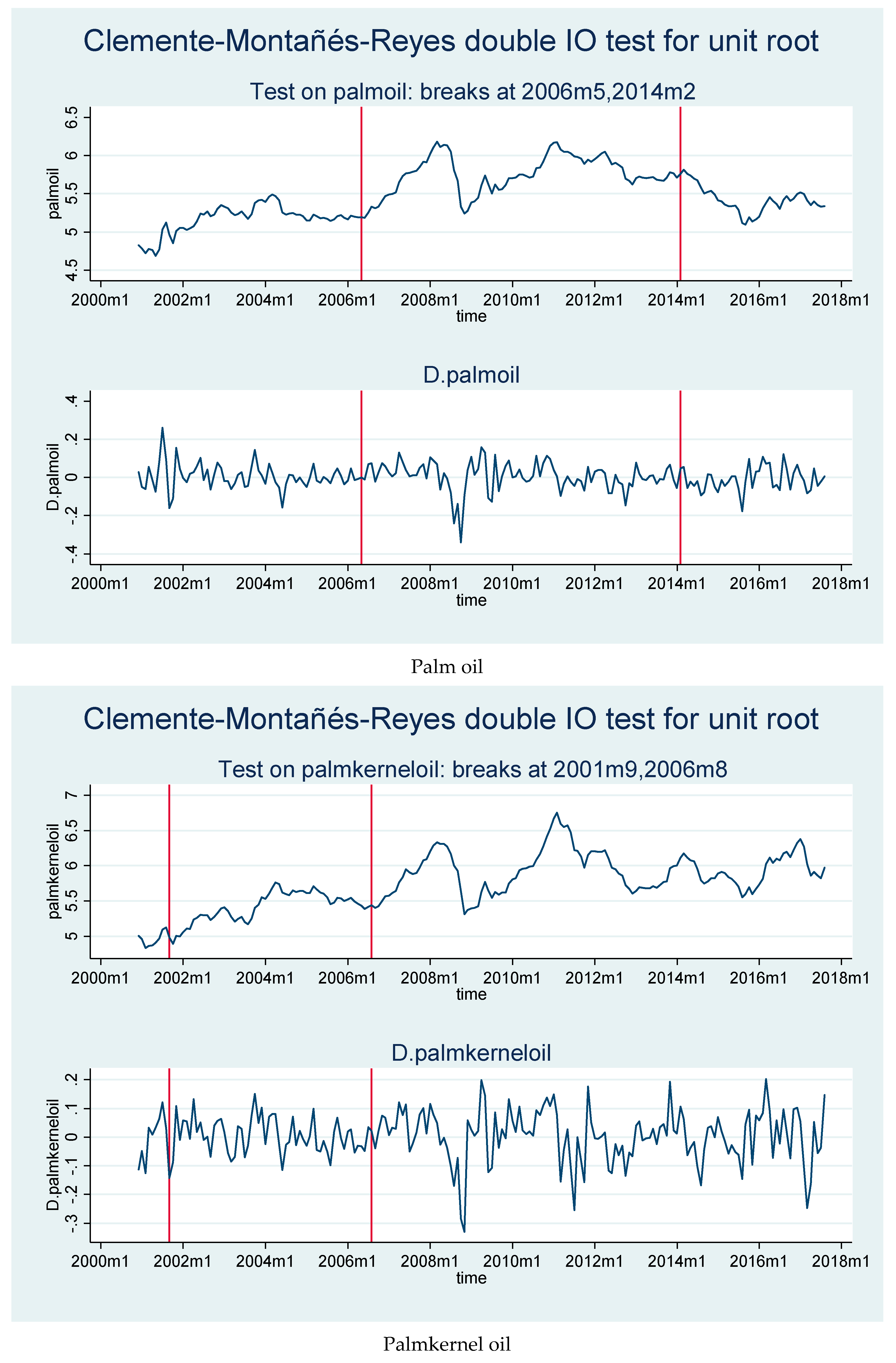
| Palm oil | −1.981 | −3.591; −4.157*; −4.282 | Intercept (2014m4); Trend (2011m1); Both Intercept and Trend (2010m8) | −4.828 | 2006m5; 2014m2 |
| Palm kernel oil | −2.379 | −5.156 **; −5.001 ***; −5.461 ** | Intercept (2012m5); Trend (2010m12); Both Intercept and Trend (2012m5) | −5.02 | 2001m9; 2006m8 |
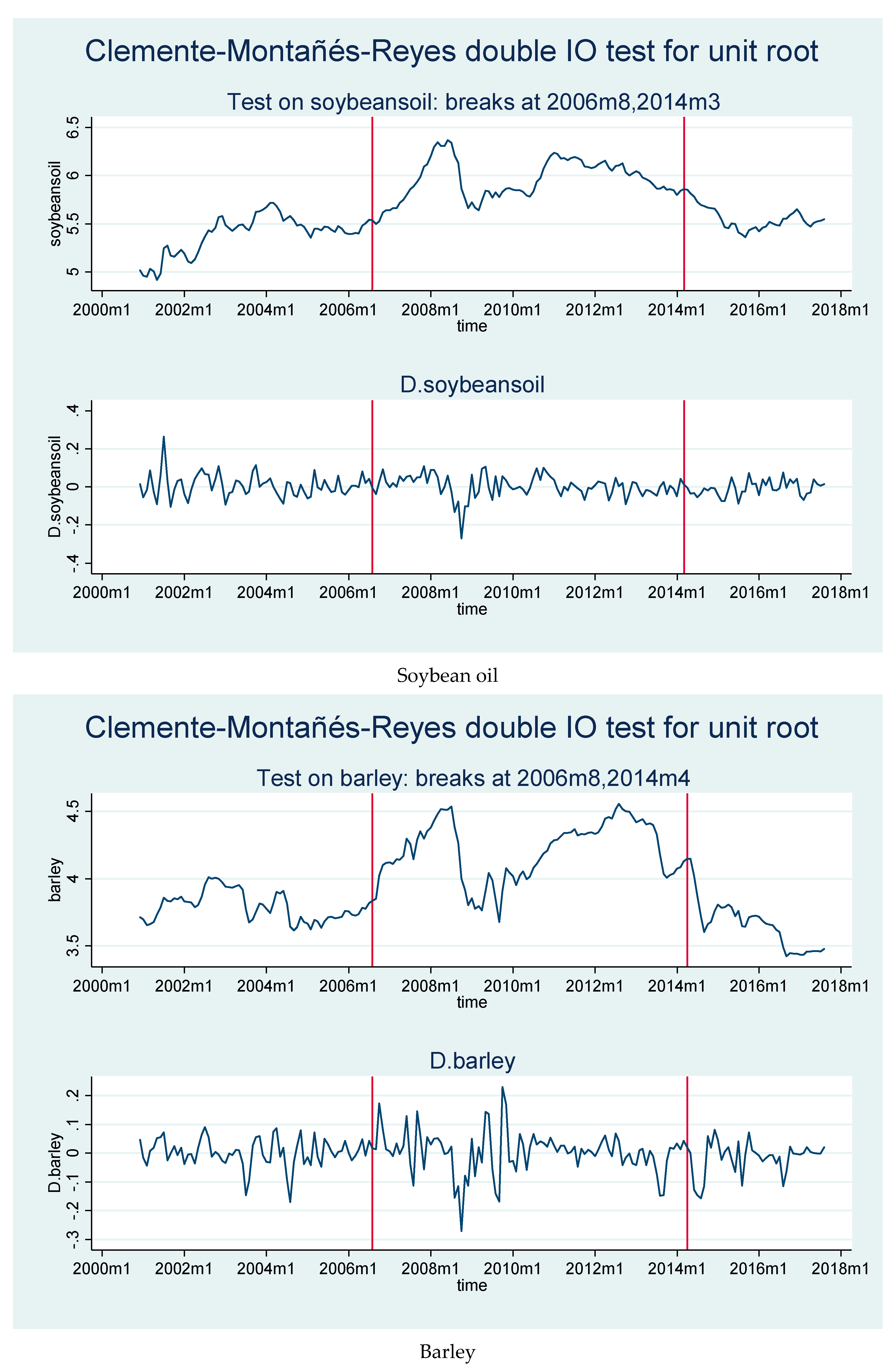
| Soybean oil | −1.729 | −2.734; −3.337; −3.515 | Intercept (2013m2); Trend (2010m12); Both Intercept and Trend (2007m4) | −4.253 | 2006m8; 2014m3 |
| Barley | −2.111 | −3.897; −3.089; −3.38 | Intercept (2014m6); Trend (2011m10); Both Intercept and Trend (2009m10) | −4.864 | 2006m8; 2014m4 |
| Cocoa | −2.381 | −3.016; −3.043; −3.376 | Intercept (2006m11); Trend (2009m11); Both Intercept and Trend (2007m12) | −4.215 | 2006m9; 2016m7 |
| Coffee | −1.734 | −3.394; −4.25 *; −4.418 | Intercept (2004m9); Trend (2011m1); Both Intercept and Trend (2012m2) | −3.929 | 2004m7; 2008m11 |
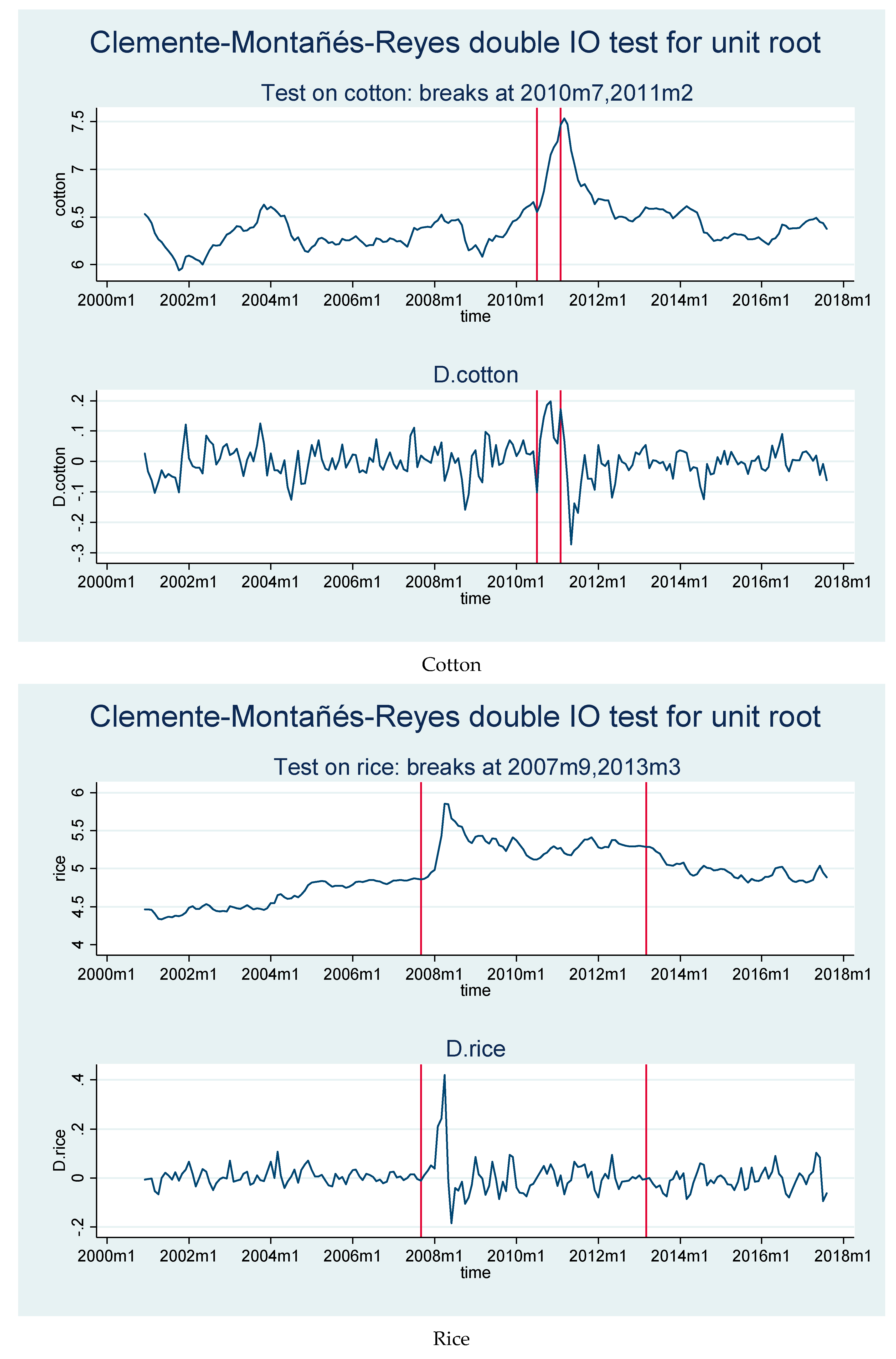
| Cotton | −2.916** | −4.042; −3.566; −4.451 | Intercept (2009m4); Trend (2010m12); Both Intercept and Trend (2010m8) | −5.505 ** | 2010m7; 2011m2 |
| Rice | −1.721 | −3.757; −4.688 **; −7.314 *** | Intercept (2013m5); Trend (2009m3); Both Intercept and Trend (2008m2) | −5.024 | 2007m9; 2013m3 |
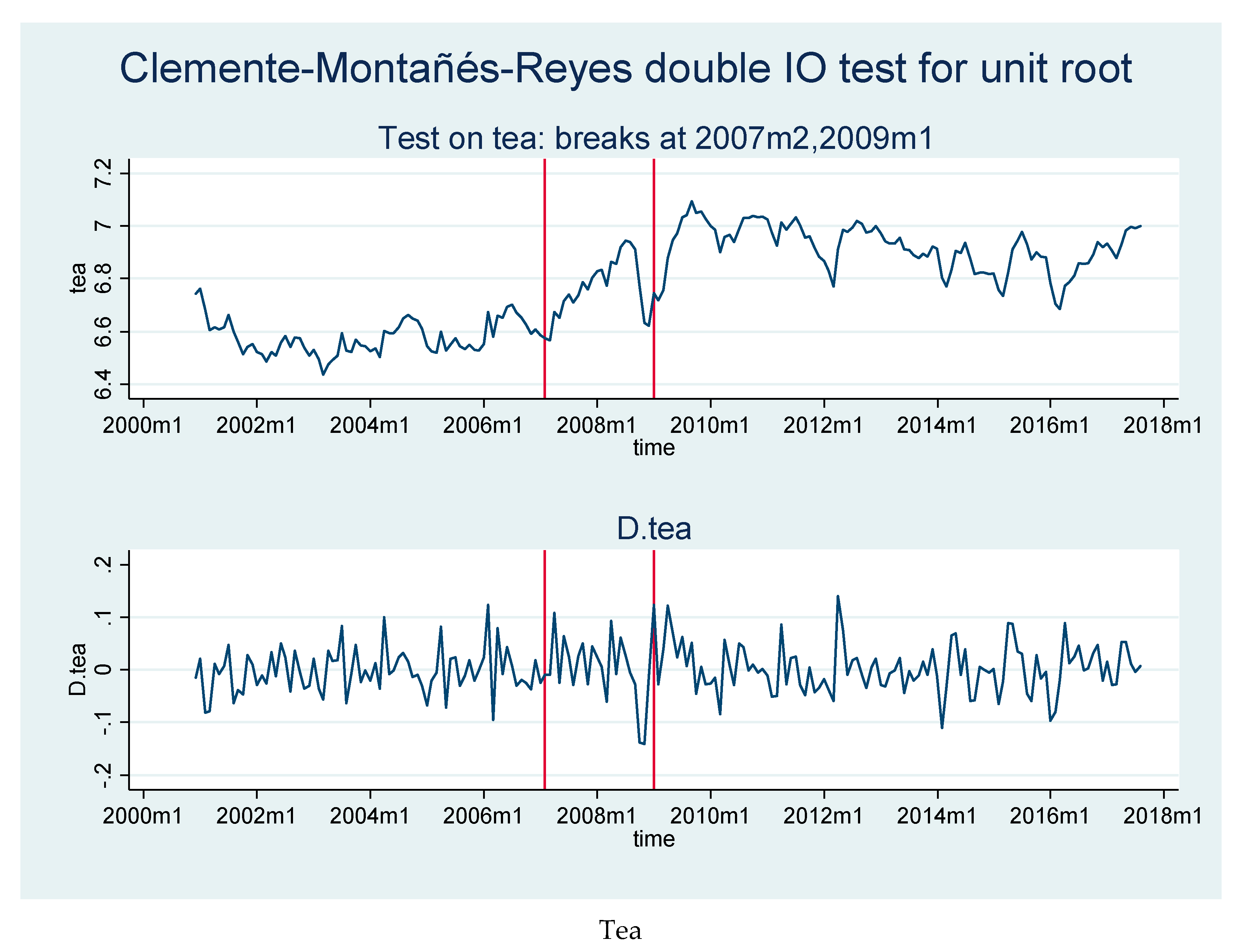
| Tea | −2.057 | −4.577; −3.545; −4.546 | Intercept (2007m4); Trend (2010m11); Both Intercept and Trend (2009m1) | −5.227 | 2007m2; 2009m1 |
| First Differences | |||||
| ADF | ZA | CMR | |||
| T-Stat | Break in | Mint t | Break in | ||
| Oil production | −10.075 *** | −13.275 ***; −13.138 ***; −13.26 *** | Intercept (2005m6); Trend (2008m10); Both Trend and Intercept (2005m6) | −4.392 | 2001m5; 2003m11 |
| Kilian’s index | −7.114 *** | −9.049 ***; −8.758 ***; −9.045 *** | Intercept (2008m6); Trend (2015m3); Both Trend and Intercept (2008m6) | −8.687 ** | 2008m8; 2008m10 |
| Brent | −9.310 *** | −12.351 ***; −12.236 ***; −12.469 *** | Intercept (2008m7); Trend (2015m9); Both Trend and Intercept (2014m7) | −8.07 ** | 2008m8; 2008m11 |
| Corn | −9.030 *** | −11.998 ***; −11.799 ***; −12.007 *** | Intercept (2012m8); Trend (2006m11); Both Trend and Intercept (2008m7) | −8.05 ** | 2008m9; 2012m6 |
| Sugar | −10.415 *** | −13.043 ***; −12.621 ***; −13.028 *** | Intercept(2008m5); Trend (2009m11); Both Trend and Intercept (2008m5) | −9.035 ** | 2008m9, 2009m9 |
| Soybeans | −6.035 *** | −6.85 ***; −6.687 ***; −7.061 *** | Intercept (2008m7); Trend(2003m1); Both Trend and Intercept (2004m4) | −7.445 ** | 2008m9; 2012m6 |
| Wheat | −9.775 *** | −12.097 ***; −11.87 ***; −12.078 *** | Intercept (2008m4); Trend (2015m9); Both Trend and Intercept (2008m4) | −6.991 ** | 2010m5; 2011m1 |
| Coconut oil | −4.706 *** | −5.538 ***; −5.328 ***; −5.521 ** | Intercept (2011m3); Trend (2015m10); Both Trend and Intercept (2011m3) | −5.855 ** | 2008m6; 2008m10 |
| Palm oil | −6.291 *** | −6.01 ***; −5.86 ***; −6.122 *** | Intercept (2008m4); Trend (2003m1); Both Trend and Intercept (2008m4) | −4.898 | 2008m6; 2008m9 |
| Palm kernel oil | −6.024 *** | −6.634 ***; −6.443 ***; −6.612 *** | Intercept (2011m3); Trend (2002m12); Both Trend and Intercept (2011m3) | −7.422 ** | 2008m6; 2008m10 |
| Soybean oil | −5.485 *** | −5.771 ***; −5.475 ***; −5.832 *** | Intercept (2008m7); Trend (2003m1); Both Trend and Intercept (2008m4) | −6.959 ** | 2008m6; 2008m11 |
| Barley | −8.509 *** | −10.003 ***; −9.899 ***; −10.159 *** | Intercept (2008m8); Trend (2015m9); Both Trend and Intercept(2013m6) | −4.353 | 2008m6; 2008m11 |
| Cocoa | −10.286*** | −13.425 ***; −13.242 ***; −13.707 *** | Intercept(2002m11); Trend(2003m7); Both Trend and Intercept (2002m10) | −13.755 ** | 2002m8; 2008m9 |
| Coffee | −9.155*** | −12.96 ***; −12.96 ***; −13.249 *** | Intercept (2011m5); Trend (2002m10); Both Trend and Intercept (2005m4) | −4.345 | 2013m12; 2014m2 |
| Cotton | −6.787 *** | −9.475 ***; −8.802 ***; −9.59 *** | Intercept (2011m4); Trend (2014m9); Both Trend and Intercept (2011m4) | −6.423 ** | 2010m6; 2011m1 |
| Rice | −8.534*** | −10.051 ***; −9.522 ***; −10.391 *** | Intercept (2008m5); Trend (2003m2); Both Trend and Intercept (2008m5) | −12.366 ** | 2007m12; 2008m3 |
| Tea | −14.410*** | −14.588 ***; −14.48 ***; −14.623 *** | Intercept (2009m10); Trend (2007m7); Both Trend and Intercept (2009m10) | −4.266 | 2008m10; 2009m8 |
| First Period | |||||||||
| ADF*Test | Zt*Test | Za*Test | |||||||
| Model | C | C/T | C/S | C | C/T | C/S | C | C/T | C/S |
| Corn | −4.067 | −5.702 ** | −4.076 | −4.216 | −4.885 | −4.204 | −24.249 | −32.949 | −25.295 |
| Sugar | −5.233 * | −5.204 | −5.475 | −5.051 * | −5.345 * | −5.412 | −33.597 | −37.511 | −41.555 |
| Soybeans | −4.451 | −4.655 | −5.01 | −4.286 | −4.521 | −4.285 | −25.269 | −28.814 | −27.719 |
| Wheat | −4.244 | −4.729 | −4.034 | −3.86 | −4.43 | −3.899 | −20.177 | −22.993 | −22.369 |
| Coconut oil | −4.329 | −4.672 | −4.292 | −4.429 | −4.893 | −5.077 | −25.751 | −29.578 | −36.886 |
| Palm oil | −4.501 | −4.69 | −4.615 | −4.648 | −4.798 | −4.782 | −31.435 | −33.816 | −34.678 |
| Palm kernel oil | −3.982 | −4.722 | −4.223 | −4.104 | −4.648 | −4.945 | −23.401 | −28.443 | −36.89 |
| Soybean oil | −5.022 * | −5.032 | −4.241 | −4.273 | −4.293 | −4.529 | −27.775 | −27.555 | −31.79 |
| Barley | −5.158 * | −5.322 | −5.647 | −4.595 | −4.716 | −4.538 | −31.032 | −31.722 | −29.661 |
| Cocoa | −4.852 | −4.731 | −4.923 | −4.985 | −4.898 | −5.007 | −37.523 | −35.73 | −37.902 |
| Coffee | −5.114 * | −5.492 * | −5.104 | −4.37 | −4.966 | −4.499 | −23 | −33.257 | −31.572 |
| Cotton | −4.213 | −4.669 | −5.026 | −4.125 | −4.725 | −4.896 | −26.629 | −34.303 | −34.407 |
| Rice | −5.149 * | −5.128 | −5.355 | −4.628 | −4.634 | −4.846 | −23.312 | −25.365 | −31.592 |
| Tea | −4.531 | −5.248 | −4.866 | −4.647 | −5.282 | −5.468 | −36.007 | −42.911 | −43.026 |
| Second Period | |||||||||
| ADF*Test | Zt*Test | Za*Test | |||||||
| Model | C | C/T | C/S | C | C/T | C/S | C | C/T | C/S |
| Corn | −5.509 ** | −5.277 | −5.396 | −6.313 *** | −5.662 ** | −6.132 ** | −37.361 | −33.266 | −36.95 |
| Sugar | −5.94 *** | −5.819 ** | −6.024 ** | −5.439 ** | −5.932 ** | −6.095 ** | −41.353 | −49.522 | −50.463 |
| Soybeans | −4.213 | −4.142 | −5.196 | −5.126 * | −4.653 | −5.524 | −25.678 | −25.131 | −33.702 |
| Wheat | −4.124 | −4.319 | −5.103 | −4.6 | −4.405 | −4.922 | −25.258 | −25.923 | −34.275 |
| Coconut oil | −4.44 | −4.452 | −4.361 | −4.232 | −4.158 | −4.252 | −20.99 | −22.344 | −25.25 |
| Palm oil | −4.939 | −4.645 | −4.997 | −4.975 | −4.541 | −4.79 | −23.895 | −23.312 | −24.359 |
| Palm kernel oil | −4.897 | −4.906 | −4.764 | −3.979 | −3.794 | −4.288 | −22.027 | −20.622 | −25.223 |
| Soybean oil | −4.333 | −4.486 | −4.66 | −5.143 * | −5.326 | −5.743 | −24.325 | −28.028 | −29.396 |
| Barley | −6.406 *** | −5.962 ** | −7.803 *** | −6.251 *** | −5.907 ** | −6.237 ** | −36.852 | −42.682 | −41.976 |
| Cocoa | −5.091 * | −5.217 | −5.12 | −4.881 | −5.031 | −5.355 | −33.844 | −35.234 | −35.184 |
| Coffee | −4.058 | −3.394 | −4.769 | −4.083 | −3.415 | −5.027 | −26.195 | −21.5 | −36.09 |
| Cotton | −3.939 | −3.652 | −4.451 | −4.17 | −3.807 | −4.371 | −24.519 | −20.969 | −27.441 |
| Rice | −4.581 | −5.099 | −5.667 | −4.431 | −4.789 | −6.784 *** | −27.063 | −32.792 | −47.299 |
| Tea | −4.806 | −5.214 | −5.533 | −4.881 | −5.152 | −5.568 | −37.077 | −39.977 | −44.11 |
| Third Period | |||||||||
| ADF*test | Zt*test | Za*test | |||||||
| Model | C | C/T | C/S | C | C/T | C/S | C | C/T | C/S |
| Corn | −6.09 *** | −6.158 *** | −6.46 ** | −4.762 | −4.765 | −6.013 ** | −28.253 | −27.232 | −46.448 |
| Sugar | −4.238 | −4.347 | −4.283 | −4.175 | −4.22 | −4.239 | −21.802 | −22.314 | −22.004 |
| Soybeans | −5.003 | −5.505 * | −5.734 | −4.847 | −5.17 | −5.645 | −33.115 | −36.889 | −41.341 |
| Wheat | −4.595 | −4.737 | −4.709 | −4.441 | −4.659 | −4.561 | −25.547 | −29.926 | −29.319 |
| Coconut oil | −3.056 | −3.211 | −4.001 | −3.022 | −3.238 | −3.826 | −18.289 | −19.887 | −26.202 |
| Palm oil | −3.872 | −4.402 | −4.866 | −3.837 | −4.237 | −4.421 | −21.874 | −28.046 | −30.517 |
| Palm kernel oil | −4.759 | −5.014 | −5.458 | −3.974 | −3.994 | −4.062 | −17.343 | −19.42 | −21.349 |
| Soybean oil | −5.261 * | −5.251 | −4.92 | −4.436 | −4.627 | −4.556 | −24.541 | −29.801 | −31.283 |
| Barley | −4.172 | −4.449 | −5.659 | −4.061 | −4.233 | −4.834 | −26.237 | −26.257 | −32.037 |
| Cocoa | −4.952 | −4.95 | −4.9 | −4.452 | −4.638 | −4.711 | −28.409 | −30.311 | −31.881 |
| Coffee | −3.941 | −4.031 | −4.592 | −3.738 | −3.892 | −4.585 | −21.45 | −22.973 | −31.257 |
| Cotton | −4.936 | −4.636 | −4.76 | −4.302 | −4.867 | −4.462 | −24.727 | −33.309 | −29.298 |
| Rice | −5.353 ** | −5.357 * | −5.254 | −4.763 | −4.764 | −4.769 | −27.068 | −28.014 | −29.973 |
| Tea | −4.499 | −4.798 | −6.026 ** | −4.403 | −4.463 | −4.894 | −25.135 | −26.476 | −34.366 |
| Direction of Causality | 2000m1–2006m7 | 2006m8–2013m4 | 2013m5–2018m7 |
|---|---|---|---|
| Corn → Brent | 0.19 | 7.79 *** | 1.3 |
| Brent → Corn | 0.96 | 1.91 | 0.04 |
| Sugar → Brent | 1.64 | 6.12 ** | 0.07 |
| Brent → Sugar | 0.39 | 0.6 | 0.07 |
| Soybeans → Brent | 1.13 | 5.24 ** | 0.05 |
| Brent → Soybeans | 2.84 | 4.33 ** | 0.91 |
| Wheat → Brent | 3.18 | 4.1 ** | 1.79 |
| Brent → Wheat | 0.83 | 0.56 | 0.07 |
| Coconut Oil → Brent | 1.04 | 8.18 *** | 0.84 |
| Brent → Coconut Oil | 3.4 | 0.11 | 0.18 |
| Palm oil → Brent | 2.11 | 9.61 *** | 0.01 |
| Brent → Palm oil | 0.89 | 2.91* | 0 |
| Palm kernel oil → Brent | 0.71 | 14.07 *** | 1.81 |
| Brent → Palm kernel oil | 2.84 | 0.001 | 0.27 |
| Soybean oil → Brent | 1.89 | 7.89 *** | 0.11 |
| Brent → Soybean oil | 3.47 | 2.11 | 0.07 |
| Barley → Brent | 1.85 | 0.44 | 0.19 |
| Brent → Barley | 0.25 | 0.53 | 0.21 |
| Cocoa → Brent | 0.41 | 1.52 | 0.88 |
| Brent → Cocoa | 0.97 | 0.59 | 0.01 |
| Coffee → Brent | 0.19 | 2.57 | 0.36 |
| Brent → Coffee | 0.15 | 0.76 | 1.05 |
| Cotton → Brent | 0.14 | 3.37 * | 0.15 |
| Brent → Cotton | 1.5 | 0.01 | 1.47 |
| Rice → Brent | 0.25 | 1.05 | 0.19 |
| Brent → Rice | 1.75 | 0.11 | 0.16 |
| Tea → Brent | 3.66 | 0.09 | 0.54 |
| Brent → Tea | 1.24 | 2.02 | 8.76 *** |
| 2000m1–2006m7 | ||||
| Oil Supply Shock | Aggregate Demand Shock | Other Oil-Specific Demand Shocks | Agricultural Price Shock | |
| Corn | 0.38 | 2.20 | 97.42 | 0.00 |
| Sugar | 0.50 | 1.80 | 97.69 | 0.00 |
| Soybeans | 0.49 | 2.47 | 97.04 | 0.00 |
| Wheat | 0.22 | 3.94 | 95.83 | 0.00 |
| Coconut oil | 0.20 | 2.57 | 97.23 | 0.00 |
| Palm oil | 0.45 | 2.66 | 96.90 | 0.00 |
| Palm kernel oil | 0.25 | 2.48 | 97.27 | 0.00 |
| Soybean oil | 0.44 | 2.30 | 97.25 | 0.00 |
| Barley | 0.74 | 2.04 | 97.22 | 0.00 |
| Cocoa | 0.47 | 1.86 | 97.67 | 0.00 |
| Coffee | 0.34 | 2.04 | 97.62 | 0.00 |
| Cotton | 0.56 | 1.88 | 97.56 | 0.00 |
| Rice | 0.46 | 2.30 | 97.24 | 0.00 |
| Tea | 0.73 | 3.22 | 96.05 | 0.00 |
| 2006m8–2013m4 | ||||
| Oil Supply Shock | Aggregate Demand Shock | Other Oil-Specific Demand Shocks | Agricultural Price Shock | |
| Corn | 0.20 | 6.47 | 93.33 | 0.00 |
| Sugar | 0.30 | 5.99 | 93.71 | 0.00 |
| Soybeans | 0.00 | 6.17 | 93.83 | 0.00 |
| Wheat | 0.01 | 5.97 | 94.02 | 0.00 |
| Coconut oil | 0.00 | 6.55 | 93.45 | 0.00 |
| Palm oil | 0.01 | 4.05 | 95.94 | 0.00 |
| Palm kernel oil | 0.00 | 6.34 | 93.66 | 0.00 |
| Soybean oil | 0.07 | 4.75 | 95.18 | 0.00 |
| Barley | 0.02 | 7.83 | 92.15 | 0.00 |
| Cocoa | 0.00 | 7.27 | 92.73 | 0.00 |
| Coffee | 0.00 | 7.75 | 92.25 | 0.00 |
| Cotton | 0.15 | 8.86 | 90.99 | 0.00 |
| Rice | 0.03 | 7.59 | 92.38 | 0.00 |
| Tea | 0.02 | 8.13 | 91.85 | 0.00 |
| 2013m5–2018m7 | ||||
| Oil Supply Shock | Aggregate Demand Shock | Other Oil-Demand Shocks | Agricultural Price Shock | |
| Corn | 6.83 | 0.23 | 92.94 | 0.00 |
| Sugar | 6.86 | 0.74 | 92.40 | 0.00 |
| Soybeans | 6.77 | 0.71 | 92.52 | 0.00 |
| Wheat | 7.65 | 0.33 | 92.02 | 0.00 |
| Coconut oil | 6.89 | 0.71 | 92.40 | 0.00 |
| Palm oil | 6.82 | 0.69 | 92.49 | 0.00 |
| Palm kernel oil | 5.59 | 0.78 | 93.62 | 0.00 |
| Soybean oil | 6.81 | 0.67 | 92.52 | 0.00 |
| Barley | 6.42 | 0.84 | 92.74 | 0.00 |
| Cocoa | 7.22 | 1.10 | 91.68 | 0.00 |
| Coffee | 6.48 | 0.63 | 92.90 | 0.00 |
| Cotton | 7.79 | 0.16 | 92.05 | 0.00 |
| Rice | 6.62 | 0.57 | 92.81 | 0.00 |
| Tea | 6.25 | 0.56 | 93.19 | 0.00 |
| 2000m1–2006m7 | ||||
| Oil Supply Shock | Aggregate Demand Shock | Other Oil-Demand Shocks | Agricultural Price Shock | |
| Corn | 3.15 | 4.19 | 92.47 | 0.20 |
| Sugar | 2.71 | 3.78 | 90.78 | 2.74 |
| Soybeans | 3.43 | 4.11 | 91.31 | 1.15 |
| Wheat | 2.98 | 5.27 | 87.92 | 3.84 |
| Coconut oil | 2.90 | 4.35 | 91.70 | 1.05 |
| Palm oil | 3.04 | 3.98 | 90.10 | 2.88 |
| Palm kernel oil | 2.97 | 4.22 | 92.00 | 0.81 |
| Soybean oil | 3.12 | 3.83 | 90.37 | 2.69 |
| Barley | 2.98 | 3.71 | 90.23 | 3.09 |
| Cocoa | 3.15 | 3.81 | 92.55 | 0.49 |
| Coffee | 3.00 | 3.97 | 92.73 | 0.29 |
| Cotton | 3.15 | 3.89 | 92.71 | 0.25 |
| Rice | 3.13 | 4.22 | 92.14 | 0.52 |
| Tea | 3.26 | 5.09 | 87.28 | 4.37 |
| 2006m8–2013m4 | ||||
| Oil Supply Shock | Aggregate Demand Shock | Other Oil-Demand Shocks | Agricultural Price Shock | |
| Corn | 0.21 | 13.95 | 76.48 | 9.36 |
| Sugar | 0.80 | 13.77 | 79.07 | 6.37 |
| Soybeans | 0.21 | 13.29 | 78.80 | 7.70 |
| Wheat | 0.18 | 12.45 | 81.18 | 6.18 |
| Coconut oil | 0.33 | 13.27 | 75.70 | 10.70 |
| Palm oil | 1.50 | 8.95 | 75.96 | 13.60 |
| Palm kernel oil | 0.34 | 12.38 | 70.26 | 17.02 |
| Soybean oil | 0.62 | 10.30 | 77.10 | 11.98 |
| Barley | 0.15 | 16.16 | 82.93 | 0.76 |
| Cocoa | 0.22 | 14.63 | 82.50 | 2.66 |
| Coffee | 0.19 | 15.82 | 80.97 | 3.01 |
| Cotton | 0.64 | 16.61 | 78.32 | 4.43 |
| Rice | 0.18 | 15.09 | 82.37 | 2.37 |
| Tea | 0.24 | 16.26 | 83.21 | 0.28 |
| 2013m5–2018m7 | ||||
| Oil Supply Shock | Aggregate Demand Shock | Other Oil-Demand Shocks | Agricultural Price Shock | |
| Corn | 19.68 | 0.44 | 77.91 | 1.96 |
| Sugar | 19.82 | 1.00 | 79.07 | 0.10 |
| Soybeans | 19.72 | 0.98 | 79.22 | 0.07 |
| Wheat | 20.30 | 0.60 | 76.98 | 2.12 |
| Coconut oil | 19.87 | 0.94 | 78.11 | 1.08 |
| Palm oil | 19.42 | 0.96 | 79.19 | 0.43 |
| Palm kernel oil | 17.04 | 1.02 | 78.11 | 3.82 |
| Soybean oil | 19.94 | 0.97 | 78.96 | 0.13 |
| Barley | 18.77 | 1.16 | 79.21 | 0.86 |
| Cocoa | 20.11 | 1.45 | 77.45 | 1.00 |
| Coffee | 19.26 | 0.88 | 79.06 | 0.80 |
| Cotton | 20.54 | 0.38 | 78.68 | 0.40 |
| Rice | 19.37 | 0.81 | 79.35 | 0.46 |
| Tea | 18.31 | 0.97 | 79.55 | 1.18 |
© 2019 by the authors. Licensee MDPI, Basel, Switzerland. This article is an open access article distributed under the terms and conditions of the Creative Commons Attribution (CC BY) license (http://creativecommons.org/licenses/by/4.0/).
Share and Cite
Vo, D.H.; Vu, T.N.; Vo, A.T.; McAleer, M. Modeling the Relationship between Crude Oil and Agricultural Commodity Prices. Energies 2019, 12, 1344. https://doi.org/10.3390/en12071344
Vo DH, Vu TN, Vo AT, McAleer M. Modeling the Relationship between Crude Oil and Agricultural Commodity Prices. Energies. 2019; 12(7):1344. https://doi.org/10.3390/en12071344
Chicago/Turabian StyleVo, Duc Hong, Tan Ngoc Vu, Anh The Vo, and Michael McAleer. 2019. "Modeling the Relationship between Crude Oil and Agricultural Commodity Prices" Energies 12, no. 7: 1344. https://doi.org/10.3390/en12071344
APA StyleVo, D. H., Vu, T. N., Vo, A. T., & McAleer, M. (2019). Modeling the Relationship between Crude Oil and Agricultural Commodity Prices. Energies, 12(7), 1344. https://doi.org/10.3390/en12071344