Modeling and Forecasting Electric Vehicle Consumption Profiles ^†

Abstract

The growing number of electric vehicles (EV) is challenging the traditional distribution grid with a new set of consumption curves. We employ information from individual meters at charging stations that record the power drawn by an EV at high temporal resolution (i.e., every minute) to analyze and model charging habits. We identify five types of batteries that determine the power an EV draws from the grid and its maximal capacity. In parallel, we identify four main clusters of charging habits. Charging habit models are then used for forecasting at short and long horizons. We start by forecasting day-ahead consumption scenarios for a single EV. By summing scenarios for a fleet of EVs, we obtain probabilistic forecasts of the aggregated load, and observe that our bottom-up approach performs similarly to a machine-learning technique that directly forecasts the aggregated load. Secondly, we assess the expected impact of the additional EVs on the grid by 2030, assuming that future charging habits follow current behavior. Although the overall load logically increases, the shape of the load is marginally modified, showing that the current network seems fairly well-suited to this evolution.

1. Introduction

1.1. Context

The car stock of electric vehicles (EVs)—electric battery and plug-in hybrids—reached 2 million units worldwide in 2016, accounting for 1.1% of the global car market share [1]. This share is expected to rapidly increase over the next 15 years. Charging an EV battery requires a large amount of energy in a small amount of time. In a typical US household, EV charging requires more power than any other appliances (e.g., stoves and dryers) and is solicited just as often (daily or more), see Figure 1. EVs are therefore important appliances to model correctly in order to manage electric household consumption. The increasing number of EVs connected to the grid, coupled with their high power requirement, is challenging the current electrical network with higher overall consumption and additional peaks.

The Nordic EV Outlook 2018, published by the Nordic Energy Research [3], gives insight into the EV market in Nordic countries (i.e., Denmark, Finland, Iceland, Norway and Sweden). In particular, the authors provide feedback from the industry in Norway, where the market share of EVs is high (1.9%), pointing out that the electrical grid experiences periodic issues in densely populated urban environments and recreational regions. This is attributed to the number of EVs charging on the grid. The Norwegian energy market regulator suggests that adding an average of 1 kW to the household peak load may result a 4% overloading of the transformers [4]. In Denmark, 20% EV penetration is believed to cause major grid overloading and under-voltage situations [5], while in the UK, a 20% level of penetration is likely to increase the daily peak load by 36% [6].

EVs are used in a multitude of contexts, including professional and leisure usage, meaning that the modeler is faced with a high and challenging variety of charging situations. Due to its nature, an EV can be charged at different places—at home or at work—which rules out a traditional switch-on appliance model. Researchers, such as Bae and Kwasinski, have proposed spatial models to account for different charging stations [7].

Modeling EV charging patterns is a useful tool for several types of study, such as power flow analyses of distribution grids [8], management of smartgrids [9], bottom-up simulations of demand [10], forecasting of charging stations [7], and stabilization of the power system [11]. Furthermore, EV charging involves a controllable load comparable to a washing machine or water heater. As such, EVs offer advantageous flexibility for demand response purposes, for instance, shifting charging cycles when electric demand is low. EV flexibility could be an important input for flexibility models, either at household level [12] or at the aggregated level [13]. Another promising perspective involves injecting the electricity stored in EVs’ batteries back into the grid, with so-called “vehicle-to-grid” projects [14].

1.2. Objective

In this study, we use data measured at high-time resolution (i.e., every minute) showing the power drawn from the grid at the charging station. Each charging station is associated with a single privately owned EV. With this data, the charging habits of each EV user are modeled in a probabilistic way. This model is described in Section 2. The charging habits model is then used for forecasting purposes: from short-term, one day ahead, to long term, in 2030.

In Section 3, we generate forecasting scenarios of an EV’s consumption profile for the next day. Although our model forecasts a single EV, we validate the scenarios at the aggregated level, i.e., for a fleet of several EVs. We observe that scenarios result in accurate probabilistic forecasts of the fleet’s aggregated consumption. In particular, we show that our bottom-up forecasting performs similarly to an advanced machine-learning method that directly forecasts the fleet’s aggregated consumption.

In Section 4, we simulate the impact of EVs on the grid in future years. The International Energy Agency (IEA) [15] anticipates a high penetration—around 30%—of EVs in 2030. Employing the four clusters of identified charging habits, we are able to extrapolate the consumption required by a large number of EVs. We show that current charging habits are sufficiently varied so as not to cause major issues on the total electrical load of a region.

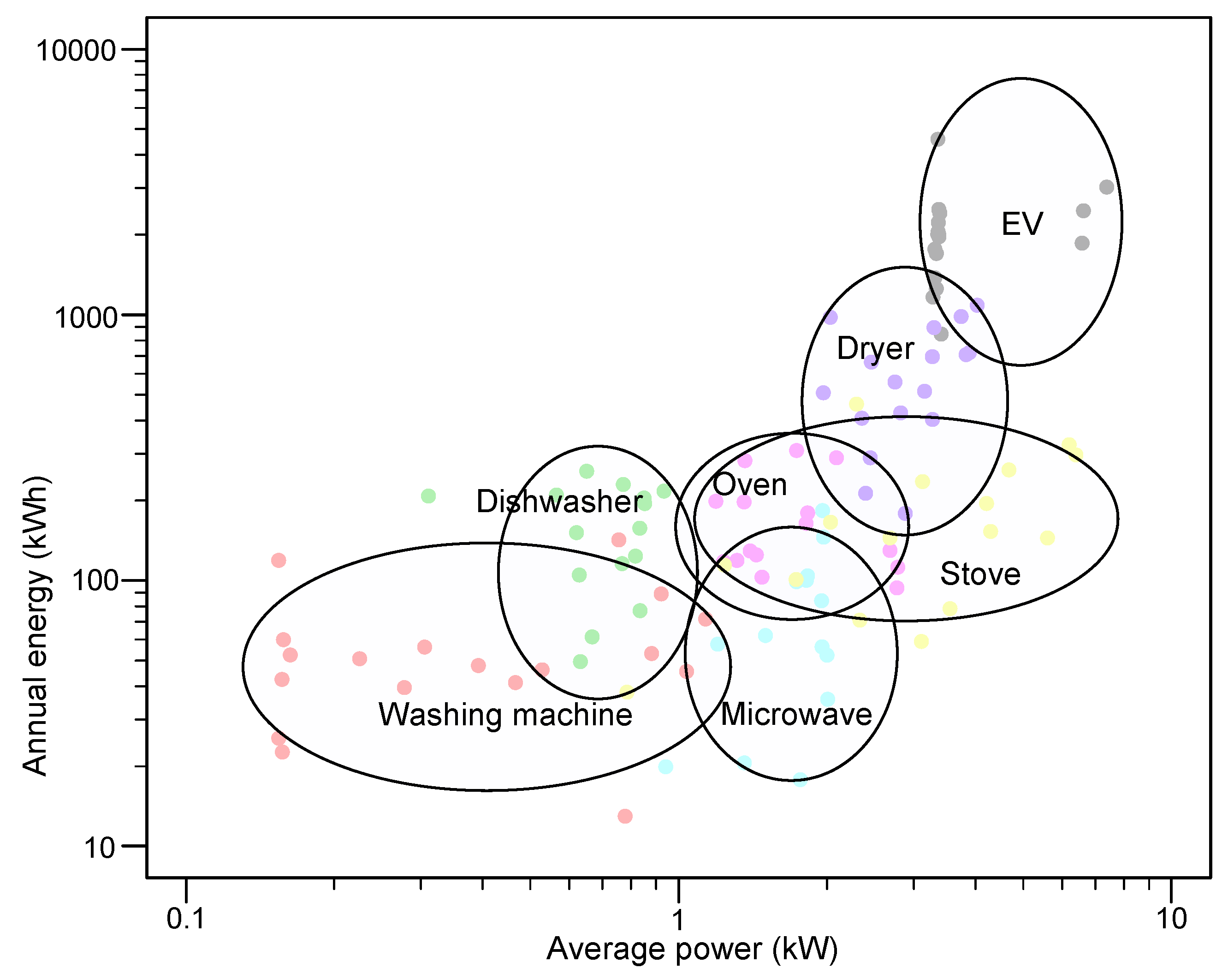
1.3. Data Description

A set of 46 privately owned EVs located in Austin, Texas, was selected. Austinites are known to be very climate conscious and supportive of green policies [16], as exemplified by the Pecan Street project run by the University of Texas [2]. The Pecan Street platform provided us with the electric consumption of each EV recorded every minute of the year in 2015. Insight into the households owning the EV was provided; houses were modern (built around 2007) and large (around 195 ${\mathrm{m}}^2$), meaning that total household consumption was high [17]. In our dataset, electric consumption related to EVs was responsible for approximately 15% of total household consumption.

2. The EV Charging Model

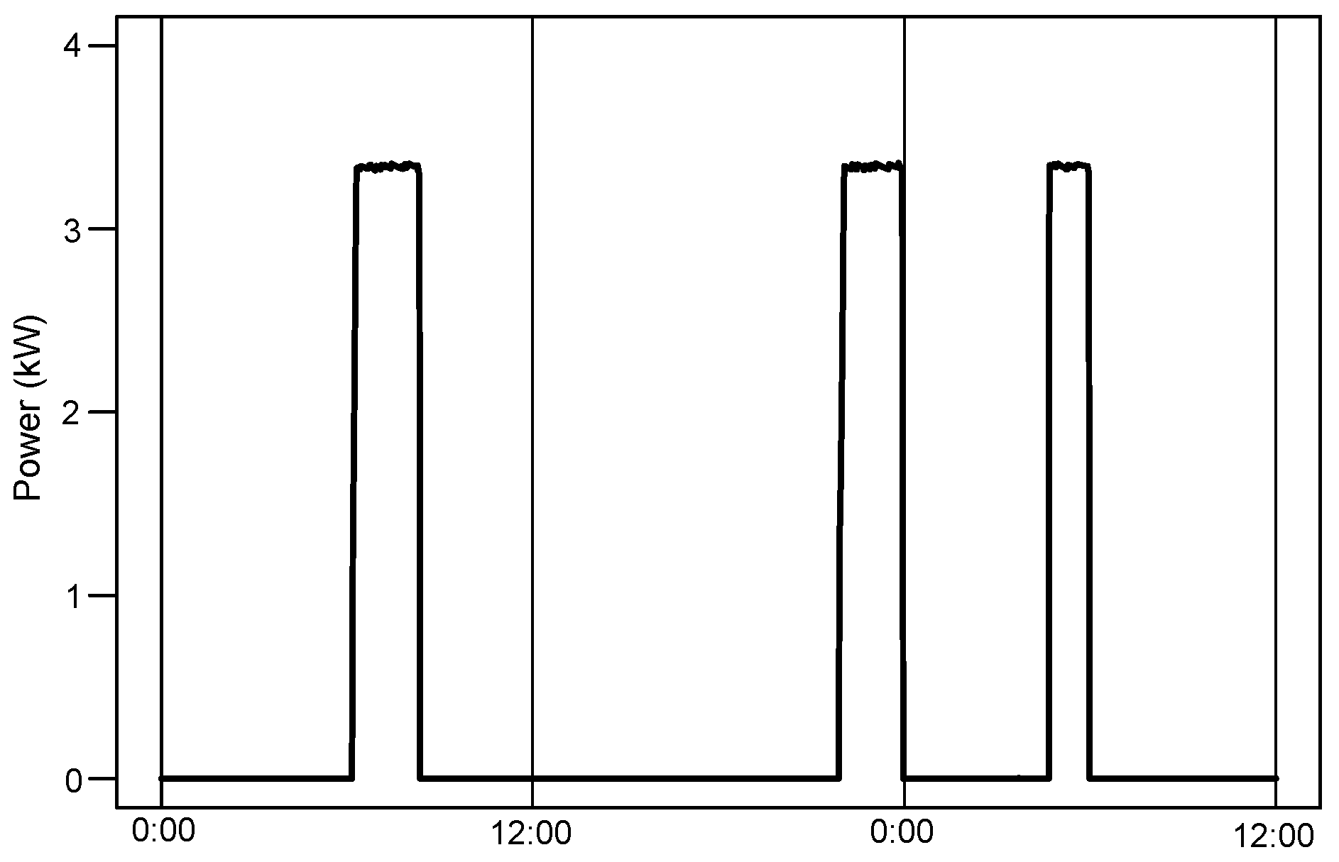
2.1. Processing the EV Time Series

An example of the power drawn by an EV during 36 successive hours is visible in Figure 2. The power drawn was either null, when the EV was not charging, or close to a specific nominal power, when the EV was charging. Based on this this visual inspection, which corresponds to the charging curve measured on a lithium-ion battery by Madrid et al. [18], we modeled a charging period with a block comprising of three parameters, see Figure 3:

• Nominal power: power demanded from the grid is constant during the whole charging period.
• Duration of the charging block.
• Start-up time: moment the day when EV charging starts (between 1 and $60\times 24$).

Real measurements did not exhibit perfect blocks. There was a steep ramp up to the nominal power; this ramp usually lasted less than 15 min. The power of the time series fluctuated slightly around a nominal value, translating a noisy phenomenon. This fluctuation was negligible compared to the nominal power, as can be seen on Figure 2. Our hypothesis of perfect charging blocks simplified these two facts.

Our observations indicate that nominal power was always the same for a particular EV as long as there was no technological replacement (i.e., battery and charging station). Such replacements occurred for two of our 46 EVs in the Austin yearlong dataset (nominal power goes from 3.5 to 6.5 kW), requiring a minor adjustment in later modeling. On the other hand, the duration and start-up time were not fixed. Charging blocks almost never started at the exact same time each day, and did not have the same duration; start-up time and duration depend on the unknown users’ habits. A realistic depiction of these habits was to describe these two parameters (duration and start-up time) in a probabilistic way. Therefore, an analysis of these parameters was required, meaning that we need to detect charging blocks on the measured power time series.

2.2. Detection of Charging Blocks

We implemented the following procedure to automatically detect the charging blocks of an EV user from the power time series:

• Detecting nominal power. The density of all of the strictly positive values was estimated, and the maximum of this density function (i.e., the statistical mode) was retrieved as the nominal power.
• Transforming time series in perfect charging blocks. The raw time series was transformed into a simpler series of two values, either 0 when power was below a threshold fixed at 50% of nominal power, or 1 when it was above.
• Pre-processing the simple time series. The time series obtained was then refined to account for measurement errors. Missing values were filled in, and any remaining blocks that were too short (less than 20 min) were removed.
• Detecting duration and start-up time. All timestamps were processed in order to list all durations and associated start-up times in the time series. The day of the year on which the charging blocks occurred was also recorded for forecast applications.

The whole procedure ran fast on an average laptop: less than 30 s for the 525,600 data points of one EV yearly time series.

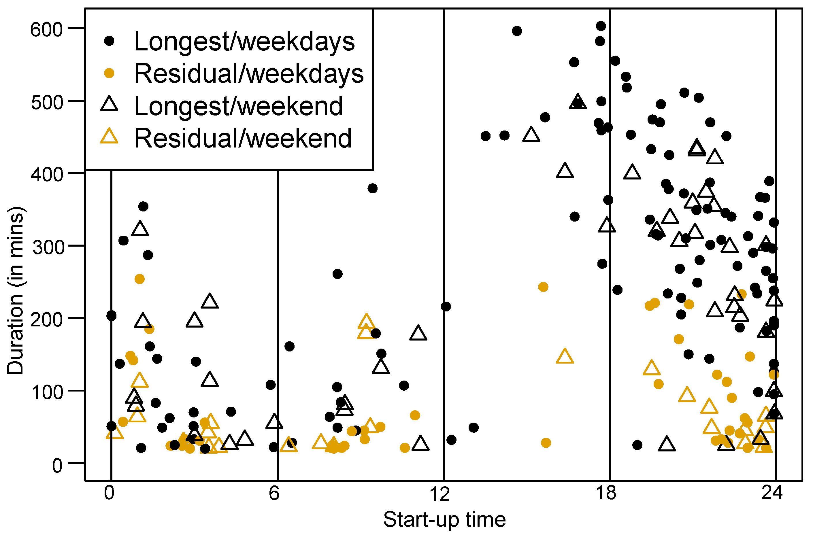
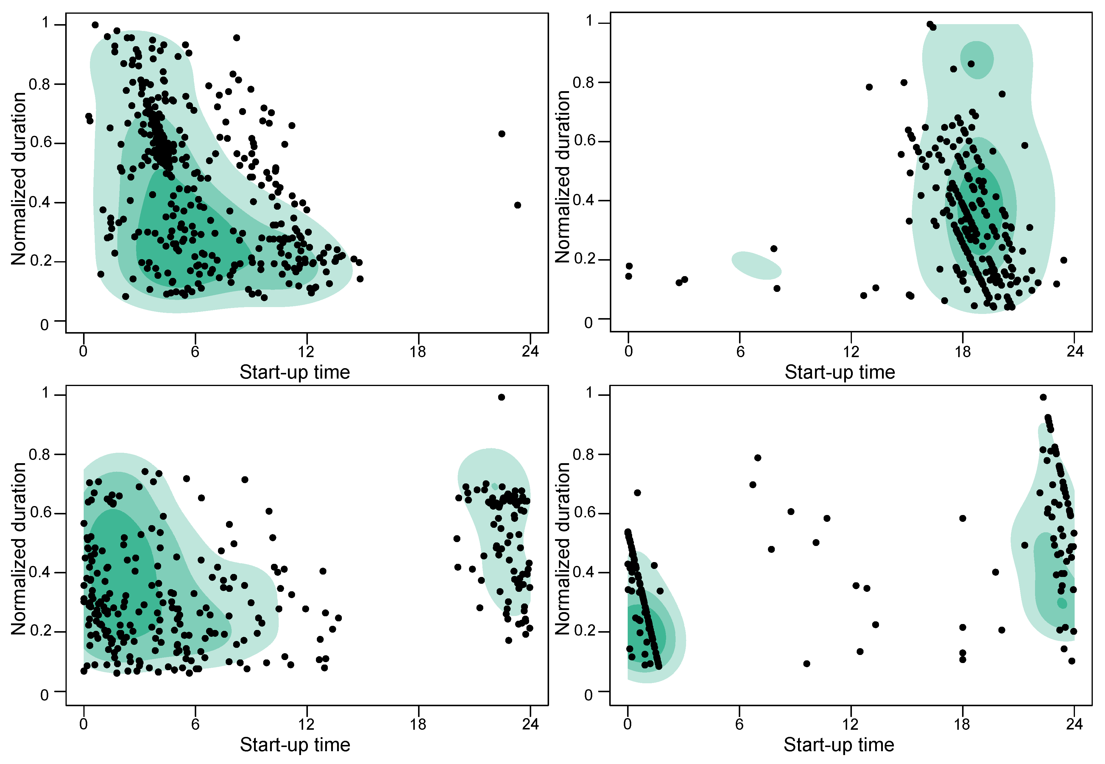
2.3. Charging Habit Analysis

Once the charging blocks parameters were detected, an analysis of the users’ charging habits was possible. An interesting representation was to superimpose every charging block of the year on a graph with the x-axis representing the start-up time, and the y-axis representing the duration of the block. In order to compare users’ habits, durations were normalized by the maximal duration observed—so that normalized duration was between 0 and 1. The maximal duration observed translates into the capacity of an EV’s battery.

Table 1. Detected characteristics of electric vehicles (EV).

Nominal Power (kW)	Max Charging Duration (min)	Battery Capacity (kWh)	Number of EVs
1.5	760	19	1
3.5	120	7	2
3.3–3.7	210–240	12–16	35
6.6	150	17	4
6.2–7.4	480–600	53–71	4

lists these maximal charging durations, the nominal power of the EVs, and an estimation of the battery capacity. Estimations of capacity matched the battery characteristics provided by manufacturers—such as the 16 kWh battery of a standard EV, or the 60 kWh battery of a premium EV. We also note that the nominal powers used to charge vehicles matched the power outputs of levels 1 and 2, i.e., slow private EV chargers described in the Nordic EV Outlook 2018 [3]. We logically observe no fast chargers ($>22$ kW and $\le 150$ kW) in our dataset, since these are mostly public and almost negligible compared to slow private chargers [3], although numbers are growing [19].

From the charging blocks detected, we detailed the number of charging cycles for each day and each EV. Data show that, on average for the 365 days of the year and one EV, there were 150 days with no cycle at all, 158 with only one cycle, and 57 with two or more blocks. Furthermore, considering only days with more than two charging blocks, the main block accounts for more than two thirds of the daily energy requirements. This shows that the main blocks are of paramount importance. Visually, see Figure 4, the characteristics of a main block and any residuals blocks (i.e., second block, third block of the day, etc.) are almost indiscernible. We ascertain this observation with a statistical test comparing the estimated density function in the 2D plan (duration × start-up time) for the main blocks and residual blocks separately, using package ks available on R software [20]. For more than half of the EVs in the dataset, p-values of the non-parametric test looking for different distribution are below 0.01 [21]. Considering these results and the fact that we observed fewer residual charging blocks, which hinders an accurate statistical model, we considered in the following that main and residual charging blocks came from the same distribution duration × start-up time.

Similar tests were conducted to determine whether weekdays and weekends follow different patterns. Perhaps surprisingly, for all EVs, we identify no statistical difference (p-value always below 0.01) in charging habits between weekdays and weekends. This is however in agreement with a visual inspection of the charging blocks’ characteristics (see Figure 4), where no clear difference stands out. It is also in line with the very low intra-week variations of the electrical load in Texas. However, despite similar habits on weekdays and weekends—EV users charged at the same time and for the same duration—we observed notable differences in the number of times that they charged their EVs each day of the week, e.g., some users almost never charged during the weekend.

2.4. Charging Habits Clustering

By making specific analysis of every user’s charging habits, we accurately describe the associated EV’s consumption profile. However, to carry out long-term forecasting requires extending these specific habits to a larger scale. We therefore aimed to cluster the charging habits to extract meaningful information that can be extrapolated in a broader context.

First, we estimated the two-dimensional density function for each EV with a kernel density estimator method; a bandwidth matrix common to all EVs was chosen and obtained with a cross-validation method [22]. Then, we compared density functions of two EVs by computing the integrated square differences on the density support. Such values defined proximity between two charging habits. Finally, thanks to a hierarchical clustering based on the Ward linkage method [23], we retrieved four habit clusters from our set of 46 EVs. These clusters represent the charging habits (start-up and duration of charging blocks) regardless of the characteristics of the vehicles, i.e., regardless of the EV’s nominal power and total energy capacity.

Table 2. Clusters found.

Cluster	Charging Period	Number of EVs	Frequency
1	Night	24	52%
2	Evening	9	20%
3	Throughout the day	9	20%
4	Late evening	4	9%

details the four clusters identified, and Figure 5 represents the two-dimensional density functions of each one of the four clusters; the green filled contours represent the density functions estimated with all users in the cluster, and the points denote the charging blocks of one randomly selected user. The first cluster (top-left) gathers the most frequent charging patterns, where EVs are charged during the night and in the morning (52% of the users). This density indicates that most charging cycles occurred before 12:00, and that cycles tended to last longer when started earlier in the night. The second cluster (top-right) gathers users charging in the evening, presumably when people come back from work (20%). The third cluster (bottom-left) gathers users charging throughout the day, but mostly at night-time (20%). The fourth cluster (bottom-right) gathers users charging in the late evening so that their vehicle is charged at a precise moment—such as 03:00 (9%). No statistical link was observed linking the characteristics of the battery and the charging patterns. Although this is in part due to the fact that most batteries are similar, we assume that the two aspects (Table 1 and Table 2) are independent.

3. Day-Ahead Forecasting Scenarios of Daily Consumption Profiles

3.1. Scenarios of a Single EV

For a specific EV, charging habits detected from the time series data allow us to forecast daily profile scenarios. This forecasting process is done in three steps:

• Forecast number of charging blocks for the next day;
• Forecast possible patterns (normalized duration × start-up time) for each block;
• Use of characteristics of the EV (maximal duration and nominal power) to obtain a consumption profile.

For step 1, the forecasting model used is a probabilistic random forest, which provided a convenient way to draw random numbers of charging blocks according to forecast probabilities, using package ranger available on R software [24].

The random forest algorithm has long been established [25] and we detail here the version implemented in the package. The algorithm trains multiple regression trees in parallel, and each tree is fitted on a different dataset. Precisely, one has a training set of K observations $b_1,\dots ,b_K$ (the daily number of charging blocks), and their corresponding inputs sets $s_1,\dots ,s_K$. Each input was made of seven elements: weekday, number of blocks one day ago, number of blocks seven days ago, median number of blocks during the seven previous days, mean temperature of the previous day. These inputs have been selected based on standard inputs for household electricity demand forecasting and empirical tests. A total of J trees, noted $w^1(·),\dots ,w^J(·)$, were to be fitted. These were standard regression trees with manually selected parameters, depth and width, to balance performance and computation time. For every tree, e.g., tree j, a random subset of 80% of the observations was used, so that, for day k, $w^1\left(s_k\right),\dots ,w^J\left(s_k\right)$ have different values. To make use of the probabilistic aspect of this model, we randomly picked only one value and rounded it to the closest integer. We manually selected a large number of trees, i.e., $J=\mathrm{10,000}$, so as to sufficiently reflect the uncertainty. For step 2, we draw patterns (normalized duration × start-up time) according to the 2D distribution observed. Forecast charging blocks were drawn from previous ones weighted by a decreasing exponential parameter $\lambda$, so that ancient blocks are forgotten. A 2D Gaussian noise, with observed covariance, is added to the block drawn. Checks are operated to rule out impossible situations; overlapping blocks, negative durations and so on.

It is difficult to assess the quality of forecast scenarios for an individual EV. Standard statistical indices (such as mean absolute error) are not adapted to such two-level time series, where the start-up times of charging blocks are highly uncertain. Forecasting methods relying on such indices lead to flat forecasts with no charging block: indeed, a correctly forecast but wrongly timed charging block—e.g., starting at 08:00 instead of 10:00—would be subject to a “double penalty” [26].

3.2. Bottom-Up Forecast of the Aggregated Fleet

Instead of evaluating forecasting performance at the individual level, the aggregated fleet consumption is forecast for the next day with a bottom-up approach. Each EV consumption profile was forecast with the three-step method described in Section 3.1, and the sum of all of the individual scenarios generates a forecast scenario for the aggregated profile. Such a day-ahead forecast is represented in Figure 6 where the aggregated profile can be clearly seen as a sum of the 46 individual EVs profiles.

To assess forecasting performance, we generated S scenarios, and turned these scenarios into probabilistic forecasts at each instant by computing quantiles at levels $\tau \in \{0.05,0.10,\dots ,0.95\}$. We compared our method with two benchmarking forecasting models that do not model individual EVs but consider only the aggregated consumption. Contrary to our bottom-up approach that forecast each individual charging before computing the aggregated load of the fleet, these benchmarks directly forecast the aggregated load, and do not consider the individual charges.

First, a persistence model using the value of the aggregated consumption at the same minute on the previous day as a forecast point (no probabilistic framework is proposed with this model). Second, an advanced benchmark is a gradient tree boosting model (GTB), with package gbm available on R software [27]. The gradient tree boosting successively combines weak classifiers to model a complex phenomenon. For regression purposes, the weak classifier is turned into a regression trees of moderate complexity. Therefore, while each tree was quick to compute, the combination of the trees was highly flexible and can model any phenomenon. We detail the algorithm thereafter. One has a training set of T observations $x_1,\dots ,x_T$ and corresponding input sets $i_1,\dots ,i_T$. An input set, e.g., $i_t$ at instant t, was made of five elements: the minute of the day, the weekday, the temperature forecast for the instant, the consumption one day ago, the median consumption during the seven previous days. These are common inputs when forecasting electricity demand [28]. The objective of the GTB is to find a function $g_{\tau }\left(i_t\right)$ that forecast a quantile value at level $\tau \in \{0.05,0.10,\dots ,0.95\}$. The level was determined by the choice of the pinball loss function ${\mathcal{L}}_{\tau }(x,y)$ defined as

$${\mathcal{L}}_{\tau }(x,y)=(\mathbf{1}(x\le y)-\tau )(y-x),$$

where $\mathbf{1}(·)$ is the indicator function. In other words, we wanted to find the function such that ${\sum }_{t=1}^T{\mathcal{L}}_{\tau }(x_t,g_{\tau }\left(i_t\right))$ was minimal. Finding the optimal function $g_{\tau }$ was made recursively for step $j=1,\dots ,J$ starting with ${}^{\left(0\right)}{g}_{\tau }\left(i_1\right)=\cdots {=}^{\left(0\right)}{g}_{\tau }\left(i_T\right)=\mathrm{constant}$. Then, for step j

• Compute the negative gradient for $t=1,\dots ,T$

  $${}^{\left(j\right)}{z}_t=-{\displaystyle \frac{\partial }{\partial g\left(i_t\right)}}{\mathcal{L}}_{\tau }(x_t,g_{\tau }\left(i_t\right)){|}_{{}^{(j-1)}{g}_{\tau }\left(i_t\right)};$$
• Fit a regression tree ${}^{j}w(·)$ forecasting ${}^{\left(j\right)}{z}_t$;
• Choose a gradient step

  $${\rho }^{*}=\underset{\rho }{argmin}\sum _{t=1}^T{\mathcal{L}}_{\tau }(x_t{,}^{(j-1)}{g}_{\tau }\left(i_t\right)+\rho w\left(i_t\right));$$
• Update estimation, for $t=1,\dots ,T$

  $${}^{\left(j\right)}{g}_{\tau }\left(i_t\right){=}^{(j-1)}{g}_{\tau }\left(i_t\right)+\rho w\left(i_t\right)).$$

Details of the regression trees, i.e., width and depth, were manually selected in order to optimize performance by the computation time reasonable. This algorithm was in practice slightly altered to improve the training process with a stochastic approach [29], i.e., only 80% of randomly selected observations are used at each step. To avoid overfitting, the number of steps is selected by cross validation.

We evaluated the forecasting quality of the three models with two standard indices: mean absolute error (MAE) for deterministic forecasts and continuous ranked probability score (CRPS) for probabilistic forecasts. Indices were estimated over a training set $\mathcal{T}$ of six months. By noting $y_t$ the actual aggregated load at instant t (to be forecast), and ${\widehat{y}}_t^{\tau }$ the forecast aggregated load at quantile level $\tau$, then

$$\begin{array}{cc}\hfill \mathrm{MAE}& ={\displaystyle \frac{1}{\left|\mathcal{T}\right|}}\sum _{t\in \mathcal{T}}|y_t-{\widehat{y}}_t^{0.5}|\hfill \\ \hfill \mathrm{CRPS}& ={\displaystyle \frac{1}{\left|\mathcal{T}\right|}}\sum _{t\in \mathcal{T}}{\int }_0^{1}2\left(\mathbf{1}\left(y_t\le {\widehat{y}}_t^{\tau }\right)-\tau \right)\left({\widehat{y}}_t^{\tau }-y_t\right)d\tau ,\hfill \end{array}$$

where $\mathbf{1}(·)$ is the indicator function. Note that if only one value is forecast (such as with the persistence model), we consider that this is the value forecast at every quantile level, i.e., the forecast distribution is a Dirac distribution. In this case, the CRPS is equal to the MAE. The obtained scores are reported in

Table 3. Indices of two benchmarking methods and our bottom-up approach.

Index	Persistence	GTB	Bottom-Up
MAE (kW)	6.24	4.86	4.87
CRPS (kW)	6.24	3.63	3.59

. Thanks to this score, we selected two meta-parameters of our bottom-up forecasts: forgetting parameter $\lambda =50$ days and number of scenarios $S=400$. Results show that our bottom-up deterministic forecasts, in addition to the decomposition of the aggregated consumption profile, greatly outperformed the persistence model, and performed similarly to the advanced GTB benchmark. Concerning the probabilistic framework, our bottom-up model was more efficient (i.e., lower CRPS) than GTB. In particular, it was notably more efficient when forecasting the lower tail of the distribution.

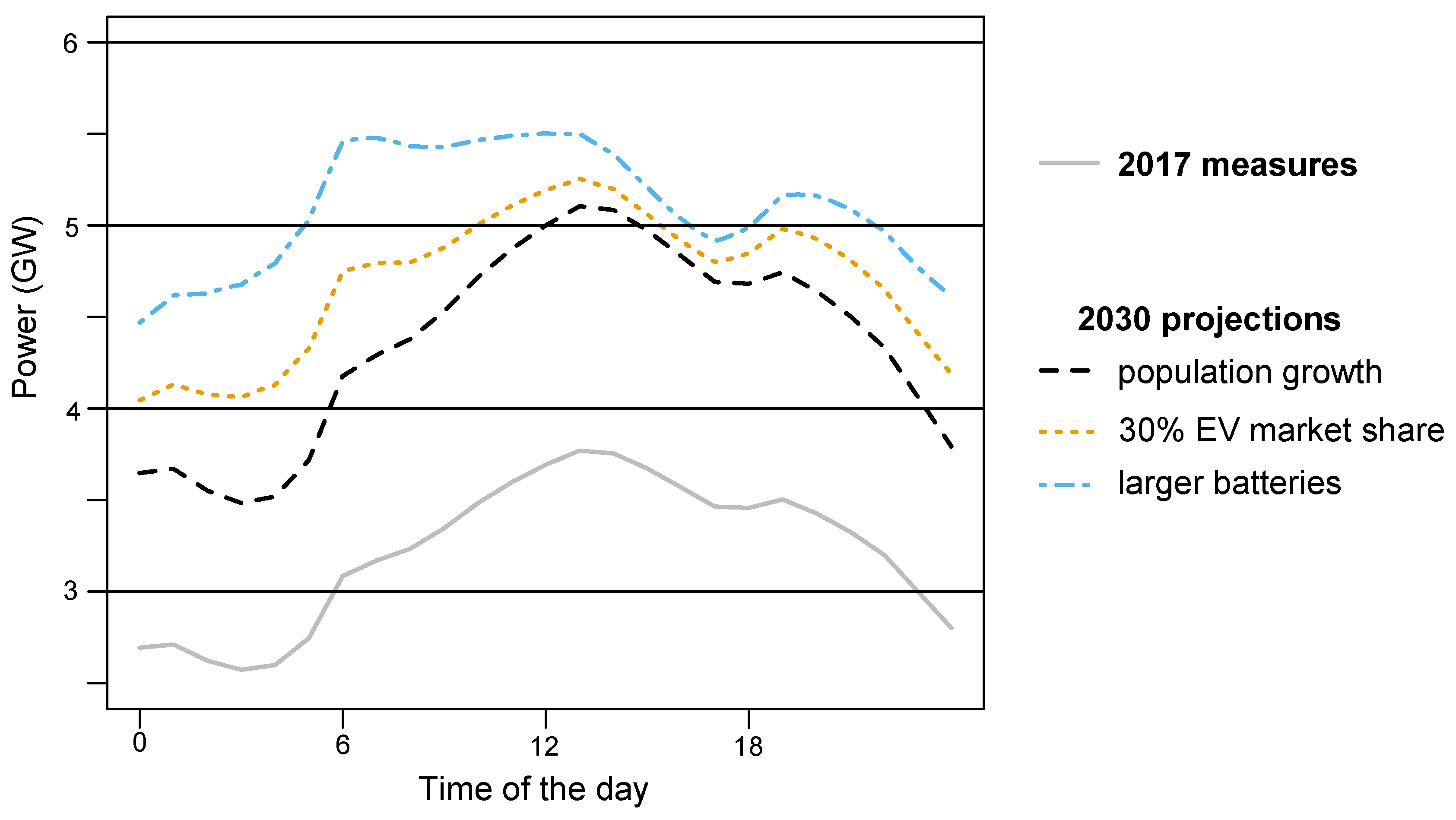
4. Long-Term Impact of High Penetration of EVs

4.1. Hypotheses

Our dataset described EV charging habits in Austin, Texas. We wanted to extend the study area to a larger region. Therefore, we focused on the South Central region of Texas. The main Texan distribution system operator, Electric Reliability Council Of Texas (ERCOT), defines this region as a weather zone covering 25 contiguous counties, comprising two major cities, Austin and most of San Antonio. According to the Texas Demographic Center, the total population of the 25 counties was 4.8 million in 2017, meaning that there were about 3.4 million vehicles. According to the 2017 National Household Travel Survey, the market share for EVs in Texas at time of writing was around 1.9%, meaning that the current number of EVs—or hybrid EVs—was around 65 thousand in the South Central region.

Considering a 1% immigration scenario in the future, the Texas Demographic Center forecasts that there should be around 6.5 million people by 2030, and thus around 4.6 million vehicles considering that the average number of vehicles per person remains the same. In addition, the IEA’s EV30@30 Campaign has set an ambitious goal of a 30% EV penetration rate by 2030. This would result in around 1.4 million EVs by 2030, which means there would be around 1.3 million additional EVs compared to the natural increase of EVs due to population growth over the period. A 30% market share is higher than that anticipated in the detailed study by Musti and Kockelman in 2011 focusing on the city of Austin [30]. These authors estimate the market share to be 19% in 2034 under a favorable feebate scenario.

4.2. Simulation

ERCOT manages electricity representing 90% of the Texan load. The company openly publishes its hourly load curve by weather zone [31]. Without any major technological changes, the load curve should have approximately the same shape in 2030, but at a higher level due to population growth. For a Tuesday in March, Figure 7 shows the actual load curve in gray, and the expected future load in black.

However, as we estimated, there should be 1.3 million new EVs charging on the grid in 2030, which will impact the load curve. We simulated all of this additional load by generating scenarios for each EV. We considered two possible evolution paths for EVs:

• Habits and characteristics of EVs remain the same (sample from complete Table 1 and Table 2)
• Habits remain the same but characteristics evolve (sample from last two lines of Table 1 and complete Table 2)

The first evolution path assumes that the habits of future users will fall with the same frequency into the four clusters found in Section 2.4, and that the EVs’ characteristics will remain the same. The second path considers the future evolution of EV chargers and batteries. Although fast or ultra-fast chargers are planned to be deployed (nominal power above 22 kW), these are expected to remain public, and public chargers are rarely used compared to private chargers due to consumer preferences. Currently, in the Nordic region, fast chargers represent less than 1% of the total charging load [32], and the growth rate of private chargers is far greater than that of public chargers [3]. However, private chargers may all reach a nominal power of 6.6 kW. We therefore retain only the last two characteristics of Table 1 with half of the future batteries of 17 kWh capacity and half in the 53–71 kWh range capacity. Evolution 1 is represented by the orange line, and evolution 2 by blue line in Figure 7.

Forecast shows that even when a high number of EVs are added to the grid by 2030, their charging only moderately impacts the shape of the load curve at the regional scale of South Central Texas. The overall load is naturally higher with the additional EVs, especially in scenario 2 with larger batteries, but the current charging habits do not cause unmanageable peaks or unstable variability for the load. Both simulations even show that, with the additional EVs, the load curve would be smoothed out during the night, diminishing the intra-day variation. With adequate planning, there should be no major problem with such market share growth. This is in line with other studies assessing the impact of EV charging, such as Luthander’s et al in a Swedish case [33]. However, since there could be issues at a local scale, some kind of coordination is required to smart-charge the EVs [6], for instance by optimally scheduling the charging of EV fleets [34], or through targeted price incentives [35].

5. Conclusions

In this paper, we model the consumption profile of EVs from raw power measurements. Based on minute-by-minute power measurements, an algorithm is developed to retrieve each charging block during which an individual charges his or her vehicle. Thanks to this detection, a probabilistic model is proposed to describe the charging habits of the user. From the measurements, we detect five kinds of plugs and EV batteries determining the power drawn from the grid and the battery capacity. Furthermore, we identify four major types of charging habits depending on the duration and start-up time of charging.

Probabilistic models of charging habits can be used to forecast the consumption profiles of single EVs for the next day through scenarios. By adding the scenarios of multiple EVs, models produce bottom-up probabilistic forecasts of the aggregated consumption of a fleet of EVs. A performance evaluation assesses that this method is as efficient as the advanced machine-learning method, but decomposes the aggregated load into single EV consumption profiles.

Since the market share of EVs is expected to greatly increase in the next 15 years, we evaluate the impact of the additional load on the total electrical load in a region in Texas with a population of around 5 million. Based on the four types of charging habits identified on our reduced dataset, we simulate the future load expected in 2030 with and without the EV market share increase, and show that it seems to only moderately impact the shape of the load curve. However, the future of EVs is uncertain, especially concerning the battery capacity and deployment of fast chargers, which may lead to complications for the grid, requiring carefully coordinated charging planning for a large number of vehicles.

References

1. International Energy Agency. Global EV Outlook 2017; IEA Publishing: Paris, France, 2017. [Google Scholar]
2. Pecan Street Inc. Dataport. 2018. Available online: https://dataport.cloud/ (accessed on 24 January 2019).
3. International Energy Agency. Nordic EV Outlook 2018; IEA Publishing: Paris, France, 2018. [Google Scholar]
4. Status of NVE’s Work on Network Tariffs in the Electricity Distribution System; The Norwegian Water Resources and Energy Directorate (NVE): Oslo, Norway, 2016.
5. Wu, Q.; Jensen, J.M.; Hansen, L.H.; Bjerre, A.; Nielsen, A.H.; Østergaard, J. EV Portfolio Management and Grid Impact Study; Annual Report; Technical University of Denmark: Lyngby, Denmark, 2009. [Google Scholar]
6. Qian, K.; Zhou, C.; Allan, M.; Yuan, Y. Modeling of load demand due to EV battery charging in distribution systems. IEEE Trans. Power Syst. 2011, 26, 802–810. [Google Scholar] [CrossRef]
7. Bae, S.; Kwasinski, A. Spatial and temporal model of electric vehicle charging demand. IEEE Trans. Smart Grid 2012, 3, 394–403. [Google Scholar] [CrossRef]
8. Putrus, G.; Suwanapingkarl, P.; Johnston, D.; Bentley, E.; Narayana, M. Impact of electric vehicles on power distribution networks. In Proceedings of the 2009 IEEE Vehicle Power and Propulsion Conference, Dearborn, MI, USA, 7–10 September 2009; pp. 827–831. [Google Scholar]
9. Mwasilu, F.; Justo, J.J.; Kim, E.K.; Do, T.D.; Jung, J.W. Electric vehicles and smart grid interaction: A review on vehicle to grid and renewable energy sources integration. Renew. Sustain. Energy Rev. 2014, 34, 501–516. [Google Scholar] [CrossRef]
10. Dickert, J.; Schegner, P. Residential load models for network planning purposes. Modern Electric Power Systems (MEPS). In Proceedings of the 2010 IEEE International Symposium, Wroclaw, Poland, 20–22 September 2010; pp. 1–6. [Google Scholar]
11. Tomić, J.; Kempton, W. Using fleets of electric-drive vehicles for grid support. J. Power Sources 2007, 168, 459–468. [Google Scholar] [CrossRef]
12. Correa-Florez, C.A.; Gerossier, A.; Michiorri, A.; Girard, R.; Kariniotakis, G. Residential electrical and thermal storage optimisation in a market environment. CIRED-Open Access Proc. J. 2017, 2017, 1967–1970. [Google Scholar] [CrossRef]
13. Ponocko, J.; Milanovic, J.V. Forecasting Demand Flexibility of Aggregated Residential Load Using Smart Meter Data. IEEE Trans. Power Syst. 2018, 33, 5446–5455. [Google Scholar] [CrossRef] [Green Version]
14. Gough, R.; Dickerson, C.; Rowley, P.; Walsh, C. Vehicle-to-grid feasibility: A techno-economic analysis of EV-based energy storage. Appl. Energy 2017, 192, 12–23. [Google Scholar] [CrossRef] [Green Version]
15. International Energy Agency. Energy Technology Perspective 2017; IEA Publishing: Paris, France, 2017. [Google Scholar]
16. Smith, C.; Fowler, M.; Greene, E.; Nielson, C. Carbon emissions and climate change: A study of attitudes and their relationship with travel behavior. In Proceedings of the Transportation Research Board’s National Transportation Planning Applications Conference, Houston, TX, USA, 17–21 May 2009. [Google Scholar]
17. Beckel, C.; Sadamori, L.; Staake, T.; Santini, S. Revealing household characteristics from smart meter data. Energy 2014, 78, 397–410. [Google Scholar] [CrossRef] [Green Version]
18. Madrid, C.; Argueta, J.; Smith, J. Performance Characterization—1999 Nissan Altra-EV with Lithium-ion Battery; Southern California EDISON: Rosemead, CA, USA, 1999. [Google Scholar]
19. Ionity. Fast Charging Station Network Starts to Take Shape: Site Partners for 18 European Countries Secured; Emobility Plus: Navi Mumbai, India, 2017. [Google Scholar]
20. Duong, T. k: Kernel Smoothing; R Package Version 1.11.1; R Core Team: Kingston, ON, Canada, 2018. [Google Scholar]
21. Anderson, N.H.; Hall, P.; Titterington, D.M. Two-sample test statistics for measuring discrepancies between two multivariate probability density functions using kernel-based density estimates. J. Multivar. Anal. 1994, 50, 41–54. [Google Scholar] [CrossRef]
22. Duong, T.; Hazelton, M.L. Cross-validation bandwidth matrices for multivariate kernel density estimation. Scand. J. Stat. 2005, 32, 485–506. [Google Scholar] [CrossRef]
23. Murtagh, F.; Legendre, P. Ward’s hierarchical agglomerative clustering method: Which algorithms implement Ward’s criterion? J. Classif. 2014, 31, 274–295. [Google Scholar] [CrossRef]
24. Wright, M.N.; Ziegler, A. ranger: A Fast Implementation of Random Forests for High Dimensional Data in C++ and R. J. Stat. Softw. 2017, 77, 1–17. [Google Scholar] [CrossRef]
25. Breiman, L. Random forests. Mach. Learn. 2001, 45, 5–32. [Google Scholar] [CrossRef]
26. Haben, S.; Ward, J.; Greetham, D.V.; Singleton, C.; Grindrod, P. A new error measure for forecasts of household-level, high resolution electrical energy consumption. Int. J. Forecast. 2014, 30, 246–256. [Google Scholar] [CrossRef] [Green Version]
27. Ridgeway, G. gbm: Generalized Boosted Regression Models, R package version 2.1.3; R Core Team: Kingston, ON, Canada, 2017. [Google Scholar]
28. Gerossier, A.; Girard, R.; Kariniotakis, G.; Michiorri, A. Probabilistic day-ahead forecasting of household electricity demand. CIRED-Open Access Proc. J. 2017, 2017, 2500–2504. [Google Scholar] [CrossRef]
29. Friedman, J.H. Stochastic gradient boosting. Comput. Stat. Data Anal. 2002, 38, 367–378. [Google Scholar] [CrossRef] [Green Version]
30. Musti, S.; Kockelman, K.M. Evolution of the household vehicle fleet: Anticipating fleet composition, PHEV adoption and GHG emissions in Austin, Texas. Transp. Res. Part A Policy Pract. 2011, 45, 707–720. [Google Scholar] [CrossRef]
31. ERCOT. ERCOT Load History. Available online: http://www.ercot.com/gridinfo/load/load_hist/ (accessed on 11 March 2019).
32. Nordic EV Barometer 2018; Norsk Elbilforening (Nordic Electric Vehicle Association): Oslo, Norway, 2018.
33. Luthander, R.; Shepero, M.; Munkhammar, J.; Widén, J. Photovoltaics and opportunistic electric vehicle charging in the power system—A case study on a Swedish distribution grid. In Proceedings of the 7th International Workshop on Integration of Solar into Power Systems, Berlin, Germany, 24–25 October 2017. [Google Scholar]
34. He, Y.; Venkatesh, B.; Guan, L. Optimal scheduling for charging and discharging of electric vehicles. IEEE Trans. Smart Grid 2012, 3, 1095–1105. [Google Scholar] [CrossRef]
35. Cao, Y.; Tang, S.; Li, C.; Zhang, P.; Tan, Y.; Zhang, Z.; Li, J. An optimized EV charging model considering TOU price and SOC curve. IEEE Trans. Smart Grid 2012, 3, 388–393. [Google Scholar] [CrossRef]
Figure 1. Annual energy (in kWh on y-axis) and average power (in kW on x-axis) of typical appliances of an US household. Source: Pecan Street [2].
Energies 12 01341 g001
Figure 2. Measured power drawn every minute by an electric vehicle (EV) during 36 successive hours. Power is null when the EV is not charging, and close to a nominal power when charging.
Energies 12 01341 g002
Figure 3. Block representation of the power drawn when charging the battery of a vehicle.
Energies 12 01341 g003
Figure 4. Each point represents a charging block of a specific EV detected during one year. Minute of the start-up time is on the x-axis, and duration of the block on the y-axis. Filled circles, or empty triangles, indicate that the charging occurred during a weekday, or a weekend day, respectively. Colors indicate if this is the longest/main block of the day or a residual block.
Energies 12 01341 g004
Figure 5. Representation of the charging patterns for the four clusters: the two dimensional density function is estimated with all the EVs of a cluster (green filled contours) and the points represent the charging block a specific EV in the cluster. On the y-axis is the normalized duration, i.e., the charging duration normalized by maximal duration observed for this EV. On the x-axis is the hour of the day.
Energies 12 01341 g005
Figure 6. Day-ahead scenario forecast of a fleet of 46 EVs on Saturday 12th December 2015. The orange dashed line shows the actual consumption to be forecast. Each individual scenario is represented by a filled area.
Energies 12 01341 g006
Figure 7. Load curves in South Central zone of Texas in a typical Tuesday in March. The grey solid line represents the load measured in 2017; the black dashed line represents the expected load in 2030 with the same EV market share (1.9%); the orange dotted line represents the expected load with a 30% EV market share and same EV characteristics as of time of writing; the blue mixed line represents this expected load with larger batteries in EVs.
Energies 12 01341 g007