Abstract
This paper proposes the development of a three-phase state estimation algorithm, which ensures complete observability for the electric network and a low investment cost for application in typical electric power distribution systems, which usually exhibit low levels of supervision facilities and measurement redundancy. Using the customers´ energy bills to calculate average demands, a three-phase load flow algorithm is run to generate pseudo-measurements of voltage magnitudes, active and reactive power injections, as well as current injections which are used to ensure the electrical network is full-observable, even with measurements available at only one point, the substation-feeder coupling point. The estimation process begins with a load flow solution for the customers´ average demand and uses an adjustment mechanism to track the real-time operating state to calculate the pseudo-measurements successively. Besides estimating the real-time operation state the proposed methodology also generates nontechnical losses estimation for each operation state. The effectiveness of the state estimation procedure is demonstrated by simulation results obtained for the IEEE 13-bus test network and for a real urban feeder.
1. Introduction
Traditionally, state estimator programs have been utilized by power system operators to remotely monitor electrical transmission systems in real time to verify whether network voltages are in compliance with national regulatory agency requirements, and, therefore, are operating under secure conditions.
In general, these transmission systems present some features that facilitate the estimation process such as fully-automated grids, meshed-grid topology, redundant sets of measurements and balanced operations. State estimator programs are integrated into the Supervisory Control and Data Acquisition (SCADA) software which provides measurement data and topological information necessary for the state estimator to work properly.
However, the reality of electrical distribution systems is quite the opposite since distribution grids present a very limited number of measurements, radial topology, unbalanced operation, and poorly-automated electrical grids. These characteristics contribute in reduction of measurement redundancy levels which may yield high errors of estimation.
In order to overcome these issues many state estimation algorithms for distribution systems have been proposed in the literature, as in [1] where Roytelman and Shaidehpour proposed a state estimation methodology to determine the state of electric power distribution systems using a minimum number of remote measurements available in power utilities. This approach uses a load flow method and a set of information about the grid as measurement data, network configuration and others to estimate the voltage magnitude and power flow values in the system.
In [2], Lu et al. addressed the problem of determining the operation state of electrical distribution systems by solving the normal equation throughout the weighted least squares (WLS) method. In this approach the authors utilized a state estimation formulation based on current equations instead of power which greatly improved the state estimation time of execution. In this formulation, the electric grid elements were represented by a three-phase model and bus voltages were considered as state variables.
Another distribution system state estimation approach was based on the use of phasor measurement units (PMUs), as proposed in [3], which are devices capable of acquiring synchronized voltage and current phasor measurements in real time. In this approach the authors also used the WLS method to estimate the bus voltage. Moreover, it is important to mention that the bus voltage was represented in Cartesian coordinates as it reduced the algorithm’s iteration number.
Conventionally, state estimation algorithms are based on node-voltage methods whereas bus voltage magnitude and phase angle are taken as state variables. However, [4] and [5] changed this perspective since they considered the branch current as state variables instead of voltage. According to the authors this modification caused an increase in the estimation process computational efficiency due to the topological characteristic of distribution grids. Furthermore, [5] also decomposed the weighted least squares (WLS) problem for the whole system into a series of WLS subproblems in a way that each subproblem is associated with a single-branch state estimation.
Despite the fact that many distribution system state estimation algorithms yield reliable results, some electrical devices such as voltage-control devices, static var compensation and others may introduce nonlinear characteristics in the objective function. This fact causes the objective equation to be non-differentiable and discontinuous which leads to convergence problems in conventional optimization techniques. Then [6] proposed a state estimator algorithm based on the heuristic method named hybrid particle swarm optimization (HPSO) to deal with this kind of problem. In addition, this method considers the presence of distributed generation (DG) and defines the active-power loads and active-power output of DG as state variables.
One of the biggest problems in distribution systems state estimation is the small amount of measurements available. This fact may lead to convergence problems in the state estimation algorithm due to lack of measurement redundancy. Faced with this situation, [7] and [8] proposed state estimation methodologies that have modeled pseudo-measurements to improve the grid’s observability. A neural network structure was used in [7] to model active and reactive power injection pseudo-measurements for the distribution systems state estimation. In this approach, the neural network’s input data were power flow measurements from load flow simulation and typical load profiles.
On the other hand, load adjustments were performed in [8] based on dynamic imbalance and utilization factors to calculate power pseudo-measurements in order to enhance the state estimator performance in distribution networks. Though this methodology is capable of estimating the voltage phasors of a distribution grid with few measurements, the utilization factor might damage the state estimation performance if it is not correctly determined.
In this context, this paper presents a methodology to estimate the state variables of electric distribution systems based on the three-phase version of the WLS conventional state estimation method, and on the proposed pseudo-measurement generation algorithm obtained from the consumers’ electric bills. This approach is able to efficiently estimate the electric distribution system operation state even considering the case when measurements records are available only at the distribution substation. To overcome this lack of recorded data, the whole feeder is featured by voltage and current magnitudes, power flows, and power injections pseudo-measurements generated by load flow simulations using the consumers’ average energy consumption bills charged monthly by the distribution utilities.
In this paper, Section 2 presents the theory and formulation regarding the three-phase state estimation based on the weighted least square approach, and the procedure used to produce the pseudo-measurements in order to ensure the electrical system full observability. The result of the proposed state estimation methodology was presented in Section 3 where this methodology was simulated in two distribution feeders: an IEEE 13-bus test feeder and the PD06 feeder, a real electric distribution grid belonging to the State of Pará Electric Utility (Brazil). The conclusions regarding the proposed approach are presented in Section 4.
2. Three-Phase State Estimation
State estimation is an important computational tool that is capable of estimating the most likely state of an electric system in real time, that is, voltage magnitude and phase angle in all nodes of the electrical network. In order to obtain the best voltage estimates, the state estimation algorithm processes a set of real-time measurements gathered from remote meters installed along the electric network. In addition, topological information regarding the electrical grid and pseudo-measurements (consumers’ historical data and other data) are also considered during the estimation process.
Although the state estimation procedure may efficiently work on transmission systems with few measurements, in general, the same result cannot be accomplished in electrical distribution systems since these systems present many features that make the state estimation procedure more challenging as: very limited number of real-time measurements, radial topology, unbalanced operation, large number of consumers, and high resistance to reactance ratio. Thus, some adjustments must be made to the state estimation algorithm in order to work on distribution systems as well.
Then, the proposed state estimation methodology attempts to overcome these issues by increasing the measurement redundancy of distribution networks, which is achieved by creating pseudo-measurements along the whole distribution feeder.
Considering these aspects, the overall structure of the state estimator program might change since the observability analysis is not necessary anymore due to the generation of enough pseudo measurements to make the distribution system full observable. In this case, the state estimator new structure is as presented in Figure 1.
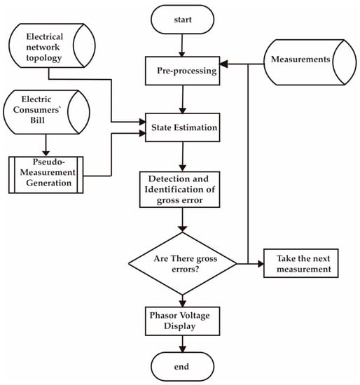
Figure 1.
Proposed State Estimation flowchart.
Despite the optimization technique be the same one as used for the single-phase state estimation procedure, the electrical devices were modeled by their three phase models as electrical distribution systems have higher levels of current and voltage imbalances that are important to be considered.
2.1. Weighted Least Square Estimation
Typically, it is considered that each measurement is made up by an expected value, which is represented in terms of state variable (voltage magnitude and phase angle), and an error as given by Equation (1):
where is the 3m x 1 measurement vector, is a 3m x 1 measurement function vector that contains the nonlinear functions that relates the measurements with the state variables, is the 3n x 1 state variable vector, is the 3m x 1 vector of error, n is the number of state variables, and m is the number of measurements by phase.
The errors reflect the corresponding uncertainty of the measurements or pseudo-measurements and are assumed to be independent to each other, i.e., one measurement does not depend of the previous one. Moreover, they are typically based on a Gaussian distribution with expected value equal to zero and variance equal to .
According to [9] and [10], the weighted least square estimator is utilized to determine the state variables of an electrical system by minimizing the weighted sum of the squared residuals as depicted by (2):
where R is diagonal covariance matrix, defined as . Moreover, according to equation (2), measurements that present larger errors tend to influence very little in state variable estimation whereas measurements with small errors greatly influence the state estimation procedure.
The weighted least squares problem is traditionally solved by the Gauss-Newton Method, which normal equation, depicted in (3), is solved in an iterative process by applying the Cholesky decomposition to the matrix and forward-backward substitutions into (3):
where is the 3n x 3n gain matrix, is the 3m x 3n Jacobian matrix, and n is the number of state variables.
The solution of (3) is the vector of increments which is used to update state variables through (4). The convergence of the state estimation algorithm is attained when is smaller than a certain specified tolerance:
where k is the iteration counter.
As depicted in (3), the gain matrix is formed by the Jacobian and covariance matrices, where the Jacobian matrix represents the sensitivity of each electrical quantity measured in relation to the state variables as shown in (5). Furthermore, the Jacobian matrix is usually structured as numerically symmetric, sparse and positive definite for fully observable networks.
where is the number of active injected power measurements, is the number of active power flow measurements, is the number of reactive injected power measurements, is the number of reactive power flow measurements, is the number of current magnitude measurements, is the number of voltage magnitude measurements, and is the number of electric nodes.
The nonlinear model is formed by the three-phase injected power models (6) and (7); three-phase power flow models (8) and (9); and the three-phase current model (10):
where p denotes phases a, b, and c, is the nodal conductance, is the nodal susceptance.
2.2. Pseudo-Measurement Generation
The major challenge in distribution state estimation is to obtain a reasonable trade-off between the number of measurements needed by the state estimator and the size of the observable area within the distribution grid, as this type of grid usually requires a significant amount of measurements for the estimator to work properly due to its radial topology, long lengths, and lack of electric monitoring along the grid.
The proposed distribution state estimation overcomes this problem by generating pseudo-measurements throughout the distribution grid, resulting in a full-observable network.
In general, the pseudo-measurement generation procedure calculates the active and reactive power flow of lines and transformers, load’s active and reactive injected power, and voltage and current magnitude in each instant of time by, firstly, carrying out a load flow simulation for an average loading condition, that is, considering the consumers’ average demand determined from the billed energy consumption, and then adjusting this demand to balance with the real-time measured injected active and reactive power at the distribution substation.
For a given radial electric distribution grid, it can be written at the substation-feeder coupling point that the average injected active and reactive power must balance total billed consumption power and total technical and nontechnical losses as presented in (11) and (12), respectively, for each phase:
where and are the average active and reactive injected power at the substation-feeder coupling point, respectively, and are the rth transformer´s equivalent active and reactive demand corresponding to the billed energy of all customers supplied by the rth transformer; , , , and are the electric network total active and reactive technical and nontechnical losses, respectively; and is the injected reactive power of shunt devices.
The customer´s average demand is obtained as in (13), and the distribution transformer´s equivalent average demand as in (14), respectively:
where is the consumer´s average active demand in kW for a time period T; is the jth consumer´s active energy consumed in kWh, T is the billing time period; N is the number of customers supplied by the rth transformer. Reactive power demand, if not measured, can be calculated by the power factor relationship.
Once calculated the active and reactive average demands of each customer along the feeder, a load flow simulation is carried out for this condition, but not including nontechnical losses, which results determine voltage magnitudes, power flows, active and reactive technical losses and , respectively, and the magnitude of injected current at the substation-feeder coupling point Imag-LF, all quantities calculated by phase.
However, these load flow results cannot be directly utilized as pseudo-measurements in the state estimator since it does not comprise the nontechnical losses expressed in (11) and (12), as, for instance, the energy theft. This fact could compromise state estimator performance because the substation measurements would not be aligned to the pseudo-measurements along the network, that is, while the substation measurements would encompass the nontechnical losses, the pseudo-measurements would not.
Then, nontechnical losses must be incorporated in the distribution transformer’s loading so that the load flow might be able to calculate power flows, current and voltage phasors more consistently. In doing so, the definition of Equivalent Operational Impedance (EOI) as presented in [11] is used. The EOI is an equivalent representation of an electric grid for the purpose of calculating technical active and reactive losses by phase, which is obtained by definition, dividing the grid total active and reactive technical losses by the rms value squared of the injected current at the substation-feeder coupling point. Applying this definition to the load flow solution obtained for the average loading condition not including nontechnical losses, as previously presented, results in equivalent operational resistance and reactance, as shown in (15) and (16):
where is the distribution feeder’s active losses calculated by the load flow simulation, is the distribution feeder’s reactive losses calculated by the load flow simulation, and Imag is the feeder’s total injected current magnitude calculated by the load flow solution. All quantities represent phase values.
The main feature of the equivalent operational impedance, that makes it appropriate for the present application, is that it is fairly constant for different loading conditions representing different operation point for the distribution grid once the electrical network topology is maintained unchanged, presenting also similar operation voltage profiles for all operation points considered [11]. Similar voltage profiles mean in a practical manner, to maintain bus voltages within (0.95 pu ≤ V ≤ 1.05 pu).
Now, applying the power balances (11) and (12) to the average loading condition previously discussed, Pinj and Qinj represent the injected average active and reactive power, measured at the substation-feeder coupling point, to supply customers´ demands connected in the distribution transformers PEr, QEr, total active and reactive technical losses PTL, QTL, and total active and reactive nontechnical losses PNTL, QNTL which are unknown. Therefore, to solve (11) and (12) the calculated Req and Xeq in (15) and (16) are used as shown in (17) and (18):
where Imag-meas is the magnitude of the measured injected phase current at the substation-feeder coupling point that corresponds to the measured injected active and reactive power Pinj and Qinj.
Once calculated the total technical losses for an electrical grid of interest for the average loading condition, the total nontechnical losses can be determined using (19) and (20):
Nontechnical active and reactive losses obtained in (19) and (20), are the missing quantities to validate the power balances represented in (11) and (12), for the average loading condition at the substation.
According to the proposed pseudo-measurement generation methodology, a load flow solution is run, starting from the average condition to calculate pseudo-measurements for the real-time state estimation algorithm. In doing so, adjustment factors are defined as in (21) and (22), for each iteration of the load flow execution [12]:
where, and are the active and reactive adjustment factors, respectively; and are the instantaneous active and reactive power injected in the substation-feeder coupling point, respectively; and k is the iteration counter. The adjustment factors are used to update the transformers’ equivalent demands, and the grid nontechnical losses using (23)–(26):
The updated values of total active and reactive nontechnical losses obtained in (24)–(26) as well as the updated values of transformers´ equivalent active and reactive demands obtained in (23)–(25) must be allocated to each individual customer in the distribution grid in order to update the grid technical losses by the load flow solution in each iteration. With respect to the transformers´ equivalent demands this is done easily by allocating the transformer´s equivalent demand variation proportionally to the customers´ actual demands. With respect to the total nontechnical losses, however, it is very difficult to identify precisely which customers are presenting irregular energy consumption patterns. So, as a reasonable solution for the purpose of pseudo-measurement generation, it is suggested that the total active and reactive nontechnical losses be allocated in the grid proportionally to the transformers loading, as described in (27) and (28):
This procedure is repeated until the convergence tolerance is achieved for the active and reactive power balance mismatches at the substation according to (29) and (30):
When the convergence tolerance is attained, pseudo-measurements of injected power, power flows, voltage and current magnitudes calculated by the load flow solution are used by the state estimator algorithm to calculate the real-time system operation state. Figure 2 depicts the flow chart that describes the steps of the pseudo-measurement generation procedure, as described previously.
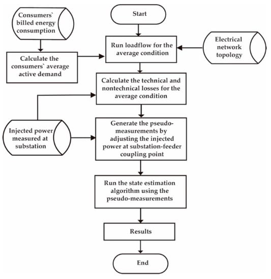
Figure 2.
Pseudo-measurement generation flowchart.
3. Results and Discussion
The state estimation methodology described in the previous sections was implemented using c++ programming language, and the OpenDSS software package was used as the load flow simulation tool, to generate pseudo-measurements to the state estimator module. Two electrical distribution grids were tested: IEEE 13-bus test feeder, and a real urban feeder.
3.1. Case I: IEEE 13-bus feeder
Initially, the proposed state estimation algorithm was tested on the IEEE 13-bus test system which represents a small-size distribution feeder. This electrical grid is radial, and unbalanced, and contains three-phase, two-phase and one-phase circuits. Figure 3 shows its single-line diagram.
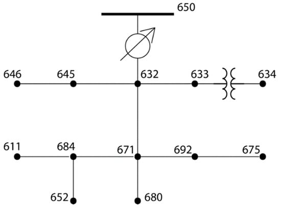
Figure 3.
Single-Line Diagram of IEEE 13-bus feeder.
The state estimation simulation was carried out on the IEEE 13-bus test feeder considering measurements only at the substation, which measured variables are voltage magnitude and injected active and reactive power by phase. On the other hand, pseudo-measurements were generated in all electric buses along the feeder according to the procedure described in the previous sections.
For simulations, it was assumed measurement errors equal to 0.1%, which is the error presented by typical measurement devices. It was also assumed that pseudo-measurement errors were equal to 1%. Measurements at substations were obtained by running load flow simulations on the IEEE 13-bus test feeder considering two operational loading conditions. OpenDSS was used as the load flow tool in the simulation studies. The presented State Estimator algorithm was programmed in C++. Moreover, the electric network parameters as line and transformer impedances were obtained as in [13]. Active and reactive loads used in the first loading condition are listed in Table 1.

Table 1.
Loads active and reactive power for average loading condition.
Voltage magnitudes estimated by the proposed state estimation algorithm for the first loading condition in phases A, B, and C are depicted in Figure 4, Figure 5 and Figure 6, for phases A, B, and C, respectively. According to these results, the state estimation algorithm was able to estimate the voltage magnitude accurately, although there were just measurements at substation.
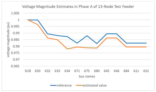
Figure 4.
13-bus feeder’s voltage magnitude estimates in phase A.
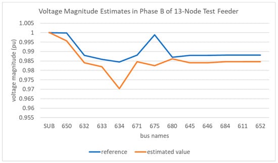
Figure 5.
13-bus feeder’s voltage magnitude estimates in phase B.
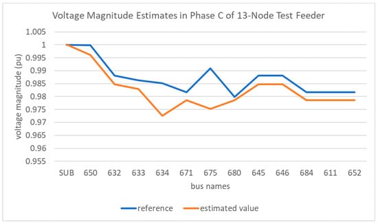
Figure 6.
13-bus feeder’s voltage magnitude estimates in phase C.
Though the pseudo-measurements presented higher errors than the real-time measurements, they played an important role in estimating the feeder’s real time operational state as they turned the network full observable, and, therefore, a solvable system.
Analyzing the voltage magnitude estimation error for the 13-bus network shown in Figure 7, it can be observed that the state estimation algorithm could estimate voltage magnitudes efficiently since 84% of the voltage estimation errors remained below 1%, while the highest errors are between 1% and 2%.
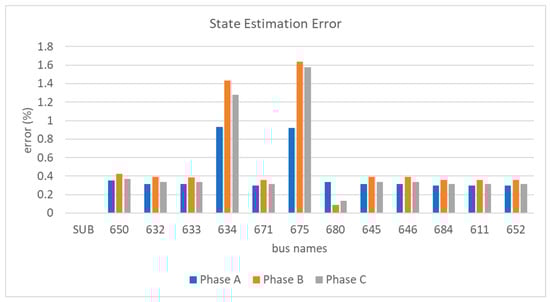
Figure 7.
Voltage magnitude error in 13-bus distribution network for the first loading condition.
The state estimation algorithm also accurately determined the active power flows in transformers and distribution lines as the obtained errors were below 1%, except in transformer T2 and line L5 where they were above 1% but less than 2% as depicted in Figure 8.
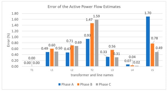
Figure 8.
Power flow error in 13-bus distribution network for the first loading condition.
Differently from what it was expected, the increase in pseudo-measurement uncertainty did not damage state estimation performance as depicted in Figure 9 since the estimation error in each electric bus along the network discretely increased with the pseudo-measurement uncertainty increase, from 1% up to 10%, which can be considered a significant error.
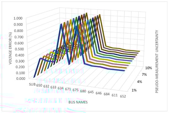
Figure 9.
Influence of the pseudo-measurement uncertainty on the proposed state estimation performance.
To test the state estimator performance for a heavier loading condition, the loads used in the previous study were considerably increased as shown in Table 2, indicating increases above 100% in some buses. For heavier load conditions it is expected that voltage magnitudes may decrease due to lack of reactive power. So, to prevent low voltage operation conditions two capacitor banks of 800 kVAr were installed at buses 632 and 671.
Table 2.
Loads Active and Reactive Power for heavy loading condition.
The state estimation simulation carried for the second loading condition converged in 3 iteration, whose total processing time was approximately 426 ms in an Intel-I5 processor, similar to the first loading condition case.
As result, it was observed that the voltage magnitude errors presented values between 0.19% and 2.58%, as shown in Figure 10, for phase A. In addition, similar results were also obtained for phases B and C.
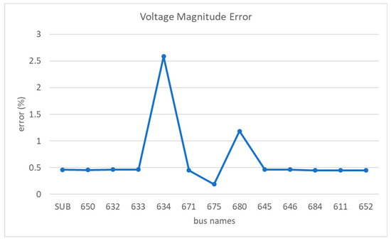
Figure 10.
Voltage magnitude error in 13-bus distribution network for the second loading condition.
Thus, the proposed state estimation algorithm is capable of determining the distribution grid’s operational state even in heavy loading conditions, which is a good indication that it can be effective in estimating the distribution grid operation states ranging from light to heavy load conditions.
Up to now, the state estimation simulations assumed that just the substation-feeder coupling point had electrical meters, and, therefore, provided measurements to the state estimator. However, electrical distribution systems usually have some devices installed along their grids as, for instance, reclosers, switches, and others, that have on-line measurements available.
The state estimator can also use the measurements provided by these types of devices to increase the network’s observability as well as the operational state estimator reliability. Besides, these measurements can highly influence the state estimation process due to be very accurate, and, therefore, present small uncertainty.
In order to evaluate how the number of electrical meters might impact the state estimator performance, some meters were gradually added to the 13-bus network. As a result, the state estimator error was reducing as soon as the number of meters increased, as shown in Figure 11. Hence, the addition of electric meters improved the result confidence.
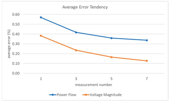
Figure 11.
Influence of adding electric meters on the estimation error.
3.2. Case II: Feeder PD-06
Feeder PD-06 belongs to CELPA, the electric utility of the state of Par–Brazil. It supplies part of the metropolitan area of Belém City, and it was chosen to test the proposed procedure in a real system. This is a three-phase 13.8 kV feeder, having 91 distribution transformers, three capacitor banks, and a total of 216 electric nodes and 123-line branches for load flow studies. Its single-line diagram is depicted in Figure 12, for illustrative purpose. The feeder data describing the electric network parameters and the load baseline used in the simulation studies performed are the same as presented in [11].
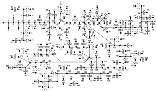
Figure 12.
Single-line diagram of PD06 feeder.
For the state estimator simulation, it was considered just real-time measurements at the substation (voltage magnitude and injected active and reactive power in phases A, B, and C), and 429 pseudo-measurements (power flows, and voltage magnitudes) along the feeder. Moreover, the real-time measurement uncertainty considered was 0.1% while for pseudo-measurements it was 10%.
As result of the state estimation simulation carried out on the PD06 feeder, Figure 13 shows that the state estimator error remained below 0.45%, which is below the pseudo-measurements uncertainty. Hence, the proposed state estimation methodology proved to be robust enough to handle large-scale distribution grids since voltage estimation error did not exceeded 1%. Although Figure 13 only shows the state estimator errors for phase A, similar results were also observed for phases B and C, been verified that maximum errors did not exceed 1%.
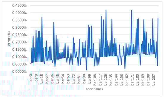
Figure 13.
Voltage magnitude error produced by the state estimator.
Similar to the voltage magnitude estimation, the proposed state estimator also determined accurately the active power flows through the PD06 feeder’s line branches since the obtained power flow errors remained within 0.01% and 1.8%, as depicted in Figure 14. Hence, this fact indicates that the state estimator efficiently determined the PD06 lines’ angular difference provided that this quantity is strongly coupled to the active power flow.
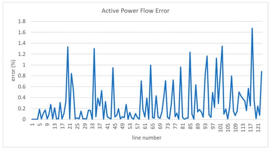
Figure 14.
Active power flow error produced by the state estimator.
4. Conclusions
The current paper proposed a three-phase state estimation methodology capable of efficiently estimating the distribution grid operation state using only measurements acquired at the substation by generating pseudo-measurements along the distribution network.
A very attractive feature of this methodology is that it works very well to obtain estimates of the operation state sufficiently accurate for practical applications using only the measurements currently available in the distribution grids, thus reducing the need for additional financial investments in new measurement devices.
Also, the proposed procedure to start the state estimation process from the feeder´s average loading condition helps to obtain the parcels of power associated with the consumed energy (paid in the energy bill), the commercial loss (consumed energy but not paid) and technical losses. Besides that, the proposed tracking procedure provides the estimates of commercial losses and billed energy for any operating point, which certainly constitutes a novelty in real time operation of distribution electrical networks.
Author Contributions
Conceptualization, T.M.S., U.H.B. and M.E.d.L.T.; methodology, T.M.S., U.H.B. and M.E.d.L.T.; software, T.M.S.; validation, T.M.S., U.H.B. and M.E.d.L.T.; formal analysis, T.M.S. and U.H.B.; investigation, T.M.S.; data curation, T.M.S.; writing—original draft preparation, T.M.S.; writing—review and editing, T.M.S. and U.H.B.; visualization, T.M.S. and U.H.B.; supervision, U.H.B. and M.E.d.L.T.; project administration, U.H.B. and M.E.d.L.T.
Funding
This research received no external funding.
Acknowledgments
The authors are grateful to CELPA – Electric Utility of the State of Pará (Brazil) by providing data from feeder PD06, via a research and development project carried out for the utility.
Conflicts of Interest
The authors declare no conflict of interest.
References
- Roytlman, I.; Shahidehpour, S.M. State Estimation for Electric Power Distribution Systems in Quasi Real-time Conditions. IEEE Trans. Power Deliv. 1993, 8, 2009–2015. [Google Scholar] [CrossRef]
- Lu, C.N.; Teng, J.H. Distribution System State Estimation. IEEE Trans. Power System. 1995, 10, 229–240. [Google Scholar] [CrossRef]
- Meliopoulos, A.P.S.; Zhang, F. Multiphase Power Flow and State Estimation for Power Distribution Systems. IEEE Trans. Power Syst. 1996, 11, 939–949. [Google Scholar] [CrossRef]
- Baran, M.E.; Kelley, A.W. A Branch-Current-Based State Estimation Method for Distribution Systems. IEEE Trans. Power Syst. 1995, 10, 483–491. [Google Scholar] [CrossRef]
- Deng, Y.; He, Y.; Zhang, B. A Branch-Estimation-Based State Estimation Method for Radial Distribution Systems. IEEE Trans. Power Deliv. 2002, 17, 1057–1062. [Google Scholar] [CrossRef]
- Naka, S.; Genji, T.; Yura, T.; Fukuyama, T. A Hybrid Particle Swarm Optimization for Distribution State Estimation. IEEE Trans. Power Syst. 2003, 18, 60–68. [Google Scholar] [CrossRef]
- Manitsas, E.; Singh, R.; Pal, B.C.; Strbac, G. Distribution System State Estimation Using Artificial Neural Network Approach for Pseudo Measurement Modelling. IEEE Trans. Power Syst. 2012, 27, 1888–1896. [Google Scholar] [CrossRef]
- Junior, M.F.M.; Almeida, M.A.D.; Cruz, M.C.S.; Monteiro, A.B.O. A Three-Phase Algorithm for State Estimation in Power Distribution Feeders Based on the Powers Summation Load Flow Method. Elect. Power Syst. Res. 2015, 123, 76–84. [Google Scholar] [CrossRef]
- Abur, A.; Exposito, A.G. Power System State Estimation: Theory and Implementation, 1st ed.; CRC Press Tayor & Francis Group: New York, NY, USA, 2004. [Google Scholar]
- Ahmad, M. Power System State Estimation, 1st ed.; Artech House: Norwood, MA, USA, 2013. [Google Scholar]
- Manito, A.R.A.; Bezerra, U.H.; Soares, T.M.; Vieira, M.V.A.; Tostes, M.E.L.; Oliveira, R.C. Technical and Non-Technical Losses Calculation in Distribution Grids Using a Defined Equivalent Operational Impedance. IET Gener. Transm. Distrib. (accepted). [CrossRef]
- Bezerra, U.H.; Soares, T.M.; Nunes, M.V.A.; Vieira, J.P.A.; Agamez, P.; Viana, P.R.A.; Oliveira, R.C. Non-technical Losses Estimation in Distribution Feeders Using the Energy Consumption Bill and Load Flow Power Summation Method. In Proceedings of the 2016 IEEE Energy Conference, Leuven, Belgium, 4–8 April 2016. [Google Scholar]
- Kersting, W.H. Radial Distribution Test Feeder. In Proceedings of the 2001 IEEE Power Engineering Society Winter Meeting, Colombus, OH, USA, 28 January–1 February 2001. [Google Scholar]
© 2019 by the authors. Licensee MDPI, Basel, Switzerland. This article is an open access article distributed under the terms and conditions of the Creative Commons Attribution (CC BY) license (http://creativecommons.org/licenses/by/4.0/).