Wind Energy Prediction in Highly Complex Terrain by Computational Fluid Dynamics

Abstract

With rising levels of wind power penetration in global electricity production, the relevance of wind power prediction is growing. More accurate forecasts reduce the required total amount of energy reserve capacity needed to ensure grid reliability and the risk of penalty for wind farm operators. This study analyzes the Computational Fluid Dynamics (CFD) software WindSim regarding its ability to perform accurate wind power predictions in complex terrain. Simulations of the wind field and wind farm power output in the Swiss Jura Mountains at the location of the Juvent Wind Farm during winter were performed. The study site features the combined presence of three complexities: topography, heterogeneous vegetation including forest, and interactions between wind turbine wakes. Hence, it allows a comprehensive evaluation of the software. Various turbulence models, forest models, and wake models, as well as the effects of domain size and grid resolution were evaluated against wind and power observations from nine Vestas V90’s 2.0-MW turbines. The results show that, with a proper combination of modeling options, WindSim is able to predict the performance of the wind farm with sufficient accuracy.

1. Introduction

In recent years, wind flow simulations have gained popularity for wind energy applications, including wind resource assessment, wind power prediction, and wind turbine micro-siting [1]. Compared to field measurements, simulations offer high-resolution three-dimensional wind fields without the need for costly meteorological equipment. Originally, linear models such as the one implemented in the Wind Atlas Analysis and Application Program (WAsP) were used because of their efficiency and their sufficient accuracy over terrain with gentle slopes [2]. However, increased computational capacity combined with a need for more accurate predictions of wind flow over complex terrain have made Computational Fluid Dynamics (CFD) models both practical and necessary. Most simulations solve the steady Reynolds-Averaged Navier–Stokes (RANS) equations, which are time independent and which provide the statistics for wind velocity at each grid point [3]. Other CFD simulation techniques that have higher accuracy, but higher computational cost are also being developed to analyze wind flow patterns and wind farm performance. These time-dependent turbulence-resolving methods include Large-Eddy Simulation (LES) and Direct Numerical Simulation (DNS). LES uses a low-pass spatial filter to average out turbulence at small length scales. In this method, the computationally-expensive calculation of small turbulent structures is replaced by sub-grid-scale modeling. One example of an LES method for wind farm modeling can be found in Porté-Agel et al. [4]. DNS involves solving the full nonlinear Navier–Stokes equations, but is too computationally expensive to be applied in large applications such as wind farms.

WindSim, a CFD package for wind resource assessment and park optimization, has been used and evaluated in both industrial settings and academia. Several groups compared the results of WindSim to WAsP over complex terrain and found better performance in the CFD model WindSim [2,5,6]. Other studies validated the WindSim results against measurements without comparing to linear models [3,7,8,9]. Castellani et al. [8,10] evaluated turbine wake modeling in wind farms with complex terrain, compared results with on-site measurements, and studied the wake effects together with the terrain effects on the performance of wind farms. Cattin et al. [7] validated the use of WindSim over areas with heterogeneous land cover, but found that implementing a map of roughness lengths did not fully reproduce the effects of forested areas. Dhunny et al. [3] validated the application of WindSim in an island situation using two roughness lengths, one for land and one for sea. Waewsak et al. [9] applied WindSim to a wind resource assessment study in Thailand and found good agreement between simulation results and met mast measurements. Finally, Teneler [11] evaluated the forest model in WindSim and found that modeling the forest as a porous medium improved simulation accuracy in heterogeneous forested regions.

The aim of the present study is to perform a more comprehensive evaluation of the WindSim software taking into account the combination of three complexities: topography, heterogeneous surface cover varying between grassy and forested, and turbine wakes. To accomplish this, we applied WindSim to a case study of a wind farm in the Jura Mountains of Switzerland, for which field data are available. We first performed convergence tests for the simulation domain size and grid resolution. We then investigated WindSim’s sensitivity to the forest model, the turbulence model, and the wake model.

2. Methods

2.1. Study Site and Data

The Juvent wind farm in the Jura Mountains of Switzerland contains 16 wind turbines, twelve 2-MW Vestas V90’s, and four 3.3-MW Vestas V112’s, with a 95-m hub height. The turbines have 90-m and 112-m rotor diameters, respectively. The turbines are situated on two hills, Mont Soleil (alt. 1291 m) and Mont Crosin (alt. 1268 m), where surface cover varies from grassy to forested (Figure 1).

Wind measurements were taken at the nacelle of each turbine from the period 15 January–11 February 2016. Data collected include wind speed, wind direction, power, yaw offset, and temperature. Each measurement was recorded as the mean over a 10-min interval. The standard deviation of wind speed over each interval was also recorded.

For the purposes of this evaluation study, only the predominant wind direction (i.e., ${240}^{\circ }$ as shown in Figure 2) was simulated. Turbines 5–8 were excluded because they were shut down for replacement during the period of analysis. In addition, we focused on the cluster of nine turbines located on the hill of Mont Crosin (Figure 1). Thus, Turbines 9, 15, and 16 were not considered in the simulations because they are far away from the nine turbines and their influences on the flow in the area of interest is negligible. Data of the nine turbines were filtered to an average wind direction of $240\pm 3^{\circ }$ and a wind speed range of 8–9 m/s as measured at Turbine 2, the farthest upstream turbine in the cluster. Wind speeds and turbine power outputs were normalized with the measurements at Turbine 2. The normalized results were then averaged over the filtered dataset because, in order to compare simulation results to observed data, we needed a single average measurement for wind speed and power at each turbine. Since Coriolis forces were assumed to be negligible in this study, normalization using linear scaling is valid [2]. Using normalized data from a certain range of wind conditions (hence, a larger dataset) allowed obtaining robust statistical results for a fair comparison.

Wind fields in mountainous regions are highly turbulent and are strongly modulated by local, nonlinear interactions with multi-scale surface heterogeneities. The complex land features of interest include both mountainous terrain and heterogeneous vegetation. In this case study, the forest-grassland mosaics of the Jura mountains exhibit land cover whose effects on wind flow are difficult to model accurately. To apply the CFD tools under such complex surface conditions, we needed to feed them with high-resolution data of the relevant surface properties. The high-resolution data of the topography is directly used as input to the CFD tools to determine the surface elevation for the generation of the computational grid. The high-resolution data of the vegetation cover can be used to estimate the surface roughness length in the similarity theory-based wall model and the parameters in the forest modeling. Forest can be modeled either directly through introducing additional forcing terms in the momentum equations or indirectly through the wall model with a high roughness length and displacement height.

In this study, elevation data at 25-m resolution were acquired from the Swiss topographical database through the www.geodata4edu.ch interface developed by the Swiss Federal Institute of Technology in Zurich (ETHZ). Land cover data at 25-m resolution were acquired from the CORINE land cover database, developed by the European Environment Agency, which classifies land cover into 44 different categories and provides the corresponding roughness length for each. Roughness length is a parameter of the vertical log-law profile that models the horizontal mean wind speed near the rough surface. It is equivalent to the height at which the wind speed theoretically becomes zero. As input to the model, we extracted from the elevation and roughness length maps a rectangular domain oriented towards the predominant wind direction (Figure 3). This ensures that the wind profile is allowed to develop over the same distance from every starting point along the inflow boundary. The dimensions of the domain were determined in a convergence test as 19 km × 5 km in the streamwise and spanwise directions, respectively, with 9-km spacing between the upstream border and Turbine 2. The elevation and roughness length presented in Figure 3 show that the Juvent wind farm is located in a highly-complex terrain. Patches with the roughness length value higher than 1 m are identified as forests, which are shown in dark red in the bottom panel of Figure 3.

2.2. WindSim

WindSim is a commercial CFD package that simulates flow over wind farms in complex terrain. The program solves the steady Reynolds-Averaged Navier–Stokes (RANS) equations using a two-equation turbulence closure model. Steady RANS simulates time-averaged flow fields assuming a statistically-stationary condition. This study focuses on the evaluation of this approach and its associated models by comparing simulation results with time-averaged field measurements. When a time average is taken, transient phenomena are smoothed out and become invisible. Hence, unsteady effects such as time-varying large-scale atmospheric forcing, topography-induced vortex shedding, and turbine wake meandering cannot be captured by steady RANS. More advanced methods (e.g., LES models) capable of capturing the unsteady effects are still too computationally expensive for commercial use in wind energy applications.

The Standard $k-\epsilon$ model (STD), the modified $k-\epsilon$ model of the Re-Normalization Group (RNG) version [12], and the $k-\omega$ turbulence model of Wilcox [13] were considered in this study. For flow over complex terrain, some studies showed that the RNG $k-\epsilon$ model produced promising results, a finding corroborated by Peralta et al. [14], while some other studies showed the superiority of the Wilcox $k-\omega$ model over the STD and RNG models [15]. Capturing the effects of forest is essential for this case study. In WindSim, forest can be modeled by the indirect approach mentioned before or by including porous cells with momentum sinks and turbulence sources [16] in the computational grid for areas that include forest. The latter is called the forest model. Our testing results (not shown) indicated that the forest model yields more realistic results than the indirect approach does. Turbine wake effects can be simulated directly by the use of an Actuator Disc (AD) model [17]. However, in WindSim, the AD model cannot be activated together with the forest model. Hence, in this study, turbine wake effects were modeled through the analytical approach. WindSim has implemented the analytical wake models from Jensen, Larsen, and Ishihara [18]. The accuracy of the three models to predict the observed power production was evaluated.

WindSim can optionally account for atmospheric stability by additionally solving the temperature equation. However, this feature requires several inputs that were not available from the measured data. Instead, we validated the assumption of a neutral boundary layer by examining the measurements. Within the selected range of wind direction and speed, we further filtered by time of day, keeping only wind events from dusk and dawn, when the atmosphere was assumed to be neutral. Comparison with the full dataset showed no significant change in time-averaged wind behavior at any of the turbines. We therefore concluded that the assumption of a neutral boundary layer for the WindSim simulations was valid for the model evaluation study here.

2.3. Boundary Conditions and Numerical Settings

The computational domain, surface elevation data, and turbine locations are shown in Figure 4. For each simulation case, the domain was rotated to make the x-axis along the prevailing wind direction, so there was only one inlet (at $x=0$) and one outlet (at $x=L_x$). At the inlet, boundary conditions are given as fully-developed flow profiles taking into account the given roughness at the border and the boundary-layer height $L_B$ [19]. For the wind speed, the well-known logarithmic profile is defined from the ground up to $L_B$, and above this height, the profile is constant. Here, $L_B$ was set to 1000 m above the mean surface elevation, and the constant speed above $L_B$ was set to 15 m/s so that the simulated wind speed at Turbine 2 was around 8.5 m/s, which is the median of the wind speed range applied to filter the data. At the outlet, zero gradient boundary conditions are imposed, meaning that a zero diffusion flux for all flow variables is assumed. On the lateral sides, symmetric conditions are applied. The upper boundary condition is specified as fixed pressure. The bottom boundary condition is no penetration together with the equilibrium log-law wall functions.

WindSim uses a Cartesian grid in the horizontal plane and terrain-following grid points in the vertical direction with tighter spacing closer to the ground level. The number of vertical grid points was set to the maximum (60). Test simulations with four different numerical settings as detailed in

Table 1. Information of the numerical settings.

Numerical Setting	Domain Size	Grid Cells	Resolution
	(${\mathit{L}}_{\mathit{x}}$, ${\mathit{L}}_{\mathit{y}}$, ${\mathit{L}}_{\mathit{z}}$)	(${\mathit{n}}_{\mathit{x}}$, ${\mathit{n}}_{\mathit{y}}$, ${\mathit{n}}_{\mathit{z}}$)	(${\mathit{d}}_{\mathit{x}}$, ${\mathit{d}}_{\mathit{y}}$, ${\mathit{d}}_{\mathit{z}}^{\mathit{min}}$)
S1	19 km, 5 km, 7.5 km	380, 100, 60	50 m, 50 m, 11.4 m
S2	27 km, 7 km, 7.5 km	540, 140, 60	50 m, 50 m, 8.4 m
S3	19 km, 5 km, 7.5 km	760, 200, 60	25 m, 25 m, 6.0 m
S4	19 km, 5 km, 7.5 km	190, 50, 60	100 m, 100 m, 11.4 m

were performed. Since the purpose of those simulations was to check the convergence of numerical results with regard to grid resolution and domain size, wake effects were not considered, and forest was modeled by the less expansive indirect approach.

For the evaluation simulations, the forest model was used. The height of the forest was set to 20 m, which is the mean height of the trees in the region according to a survey [20]. The number of grid cells in the vertical direction for modeling the forest was set to five, corresponding to $d_z^{min}=4$ m. According to the table in WindSim, the forest resistive force constant $C2$ was set to 0.01, twice that of the default value, because the forest at Mont Crosin was sparse, but dominated by Picea abies and Abies alba, which are evergreen coniferous trees with a higher leaf area index. The influence of $C2$ on the results is presented in the next section.

3. Results and Discussion

Figure 5 shows the normalized wind speeds at the hub height of turbines predicted by WindSim using the standard $k-\epsilon$ model with the four different numerical settings defined in Table 1. It can be seen that the differences between the results of these numerical tests (except for S4, which had the coarsest grid resolution) were rather small. This indicates that the results presented in the following with the numerical setting S1 did not depend on the domain size and grid resolution. S1 (medium grid resolution) was ultimately chosen because it produced results much faster than using S3 (fine grid resolution). Furthermore, the nesting technique (using the results from a larger outer model with coarser resolution as boundary conditions for flow simulation over a smaller domain with higher resolution) was also tested for S1. The nested simulations did not further change the results (not shown). Therefore, the influence of inaccuracies in the assumed boundary conditions on the results of S1 can be regarded as negligible.

Normalized turbine power outputs predicted by WindSim using three different turbulence models are compared with the wind farm SCADA data in Figure 6. Here, the analytical wake model of Ishihara was used, and the effect of multiple wakes was modeled by the linear superposition of the wake deficits. The predicted power outputs were obtained for three incoming wind directions (${237}^{\circ }$, ${240}^{\circ }$, and ${243}^{\circ }$) and different wind speeds (around 8.5 m/s) at the reference turbine, then averaged to yield the mean values and standard deviations (error bars). It is shown that the results of Wilcox were all within the error bars of the data, while the results of STD and RNG largely under-predicted the power outputs of Turbines 1, 11, and 12. To have a quantitative measure of the model performance, the Root Mean Squared Error (RMSE) and Mean Bias (MB) were calculated as follows:

$$\mathrm{RMSE}=\sqrt{\frac{1}{N}\sum _{n=1}^N{(P_s^n-P_o^n)}^2}$$

(1)

$$\mathrm{MB}=\frac{1}{N}\sum _{n=1}^N(P_s^n-P_o^n)$$

(2)

where $P_s^n$ is the simulated mean power output of turbine n, $P_o^n$ is the observed mean power output of turbine n, and N is the number of turbines used for comparison. RMSE was 0.09 for the Wilcox model, 0.20 for the STD model, and 0.25 for the RNG model. MB was almost zero for the Wilcox model, −0.15 for the STD model, and −0.20 for the RNG model. Overall, it can be concluded that the Wilcox model outperformed the other two models in terms of predicting turbine power outputs in complex terrain.

To have a closer look at the different behaviors of the turbulence models, we plot the fields of predicted wind speed at the height of 95 m for the predominant incoming wind direction in Figure 7. It turns out that at the leeward side of the first hill (marked by the black triangle), where Turbine 2 is located, wind speeds predicted by the Wilcox model were lower than those predicted by the STD model and the RNG model. Since the power of Turbine 2 was used to normalize the results, this explains why the STD and RNG models tended to underestimate the normalized powers at the other turbines. This finding is consistent with other studies showing that the Wilcox model is able to predict mean velocity and turbulent kinetic energy that are closer to the measurements than the other models [15]. The Wilcox model involves the solution of transport equations for the turbulent kinetic energy k and the specific dissipation rate $\omega =\epsilon /k$ where $\epsilon$ is the dissipation rate of k [13,21]. Compared to the $k-\epsilon$ models, the $k-\omega$ model has several advantages, namely that: (1) the model is reported to perform better in mildly-separated flows; (2) the model is numerically very stable; (3) the low-Reynolds-number version is more economical and elegant in that it does not require the calculation of wall distances, additional source terms, and/or damping functions based on the friction velocity. It can be inferred from the results that, among those advantages, the first one is mainly responsible for the best performance of the Wilcox model found here.

With the Wilcox turbulence model, the performances of the three analytical wake models implemented in WindSim were evaluated. Again, the linear superposition of velocity deficits was adopted to handle the multiple wakes. As shown in Figure 8, among the three wake models, the Ishihara model yielded the best overall results with an RMSE being 0.09 and an almost zero mean bias, while the Jensen model had an RMSE of 0.15 and an MB of −0.08, and the Larsen model had an RMSE of 0.21 and an MB of 0.10. The better performance of the Ishihara model may be due to the fact that it introduces a turbulence-dependent rate of wake expansion and adopts the Gaussian shape for the velocity deficit. Nevertheless, it is important to note that none of these analytical wake models considers the change of wake growth with topography due to the pressure gradient, which could be significant according to a recent study [22].

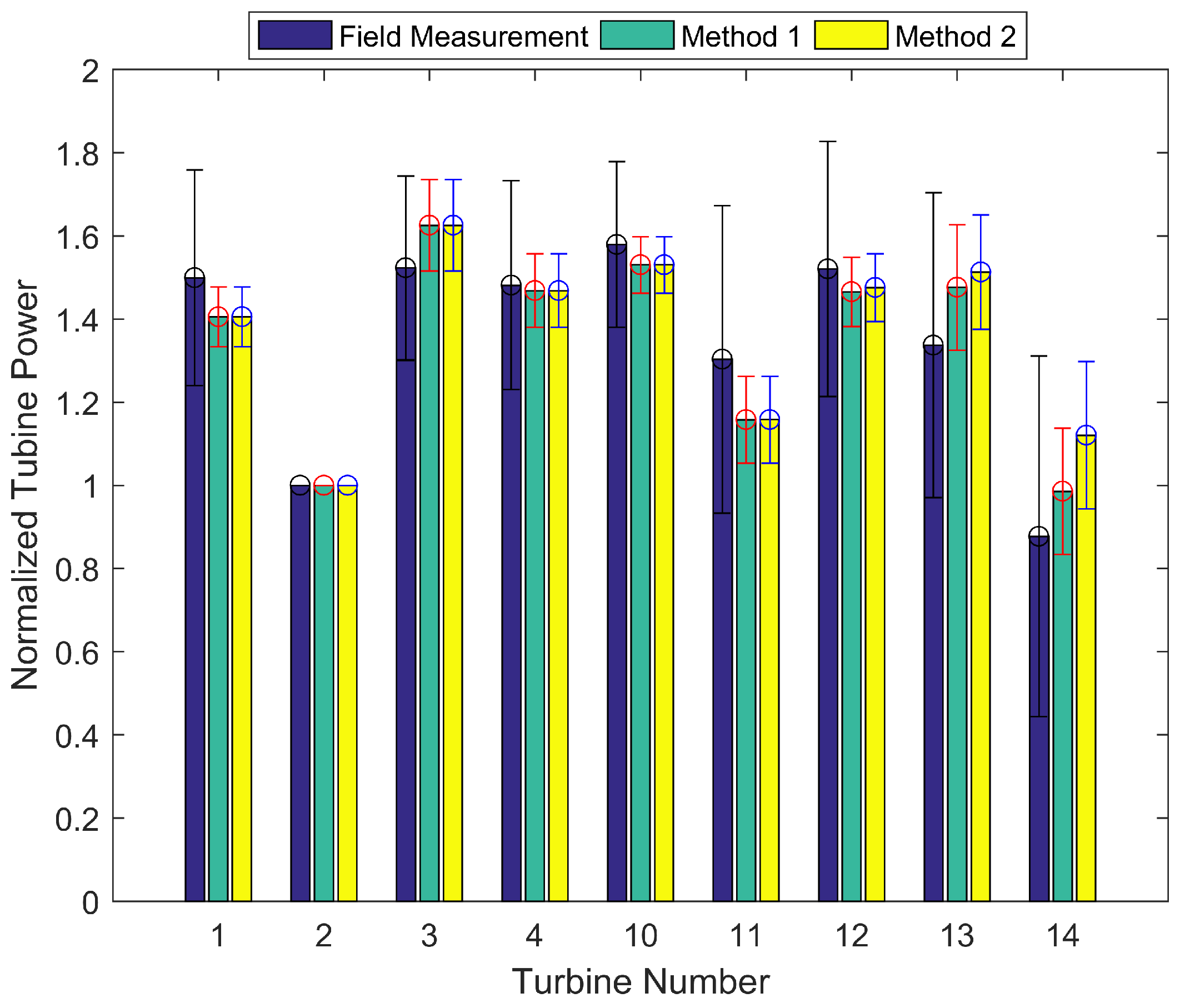
Figure 9 compares the results obtained by using two different approaches to calculate the superposition of multiple turbine wakes. It turns out that the linear superposition approach led to stronger multiple wake deficits for the last two downstream turbines (13 and 14) and predicted normalized powers that were in better agreement with the measurements, compared with the other approach that uses the square root of the sum of the squares of the velocity deficits. It is worth mentioning that similar behaviors of the two approaches were found in a study of the Horns Rev offshore wind farm [23].

Table 2. Data of the RMSE and Mean Bias (MB) of the predicted normalized powers for the model combinations.

Combination	Turbulence Model	Wake Model	Multiple Wakes	RMSE	MB
C1	Wilcox	Ishihara	Method 1	0.09	0.00
C2	STD	Ishihara	Method 1	0.20	−0.15
C3	RNG	Ishihara	Method 1	0.25	−0.20
C4	Wilcox	Jensen	Method 1	0.15	−0.08
C5	Wilcox	Larsen	Method 1	0.21	0.10
C6	Wilcox	Ishihara	Method 2	0.12	0.02

summarizes the prediction errors of the various combinations of modeling options. It is evident that the $k-\omega$ turbulence model of Wilcox together with the analytical wake model of Ishihara and the linear superposition of multiple wake deficits yielded the best performance. Some other combinations of turbulence and wake models were also tested (results not shown), and none of them outperformed the one recommended above. Nevertheless, for this case study, the forest modeling played a key role, and the results were sensitive to the choice of the forest resistive force constant $C2$, as shown in Figure 10.

4. Conclusions

The capability of the CFD software WindSim to predict the power outputs of the wind turbines of a wind farm over complex terrain was evaluated in this study. The site of the case study featured the co-presence of three complexities: topography, heterogeneous vegetation with a woodland-grassland mosaic, and interactions between wind turbine wakes. Hence, it allowed an in-depth evaluation of CFD models. The outcome of this study can be concluded as follows:

• The WindSim modeling setup using the $k-\omega$ turbulence model of Wilcox together with the analytical wake model of Ishihara and the linear superposition of multiple wake deficits was able to simulate turbine power outputs that were in good agreement with the measurements in this case study.
• Simulation results were sensitive to the choice of modeling schemes and parameters, especially the analytical wake model and the resistive force constant $C2$ in the forest model. Therefore, more validations at different sites of complex terrain are needed before generalizing the optimal modeling setup found in this study.

Comparison with more advanced models such as large-eddy simulation together with actuator disk model would help to verify that the good agreement was not due to the offset of various modeling errors discussed in the paper. Moreover, for forested mountainous regions, high-resolution terrain and vegetation data such as canopy height and density are needed to estimate accurately the relevant parameters for numerical wind energy prediction.