1. Introduction
Robot manipulators are often used in various industries, such as packaging and automotive manufacturing. A robot manipulator’s dynamic behavior is entirely nonlinear, coupled, and time-variant, which causes several challenges in fault detection, estimation, identification, and tolerant control. Heavy-duty cycles, overloading, poor installation, and operator errors can be caused by various defects: Sensor faults, actuator failures, and plant faults [
1,
2,
3].
Several types of fault diagnosis and fault-tolerant control algorithms have been developed for robot manipulators. These methods are divided into four main classes: (a) Signal-based, (b) model-reference, (c) knowledge-based, and (d) hybrid techniques [
4,
5,
6]. All methods for fault diagnosis have specific advantages and challenges. Signal-based fault diagnosis extracts the main features from output signals. Because of the presence of disturbances, the performance of this method is degraded. Knowledge-based fault diagnosis is highly dependent on the historical data used for training, which incur high computational costs for real-time data. The model-reference method identifies faults using a small dataset, but it requires an accurate system model [
7]. Hybrid fault detection, estimation, and identification techniques use a combination of high-performance methods to design a stable and reliable technology [
8]. In this paper, an intelligent model-reference (hybrid) technique is proposed for fault detection, estimation, and identification.
The core of this study was observer-based fault detection, estimation, and identification. System modeling was divided into two principal techniques: (a) Physical-based system modeling, which uses a disassembled robot manipulator to extract the Lagrange mathematical formulation, and (b) signal-based system identification, which uses various identification techniques. To address the challenges posed by the complexities and disturbance problems of physical-based system modeling, we used a signal-based system identification technique based on the autoregressive exogenous input (ARX)–Laguerre technique [
9,
10,
11].
Various observer-based techniques have been used for fault detection, estimation, and identification, and they are divided into two main groups: (a) Linear-based observers and (b) nonlinear-based observers [
10]. Proportional integral (PI) observers are linear and have been used in different systems for fault diagnosis, but they are ineffective in the presence of uncertainties and disturbances [
12]. To address those issues, nonlinear observers (e.g., adaptive, sliding mode, feedback linearization, and fuzzy) have been introduced [
10,
13,
14,
15]. Feedback linearization observers are stable; however, they are not adequately robust [
14]. Sliding mode observers are robust and stable, but chattering is the main drawback of this technique for fault diagnosis in the presence of uncertainties [
10]. The fuzzy logic observer has an acceptable state estimation and works in uncertain conditions; however, reliability is the main drawback of this technique [
15]. Among the available options, hybrid methods provide the most suitable techniques for fault detection, evaluation, and identification in a robot manipulator.
Linear and nonlinear fault-tolerant control algorithms are the main techniques for reducing or eliminating the effects of faults in robot manipulators. Coupling effects and an increase in the gear ratio are the main drawbacks of linear fault-tolerant control algorithms [
16]. Model-reference fault-tolerant algorithms, knowledge-based techniques, and hybrid fault-tolerant control methods are the main techniques used in robot manipulators [
16,
17]. Model-based and knowledge-based fault-tolerant control algorithms have several advantages, such as system knowledge, stability, robustness, and reliability, but they face a big challenge in the unlimited level of a faulty signal [
17]. Hybrid fault-tolerant algorithms are used to address that issue [
18,
19]. The sliding mode technique can be an excellent candidate for a robust fault-tolerant control algorithm, but it must address the challenge of chattering. Various techniques have been proposed to attenuate chattering [
16,
17,
18,
19]. An adaptive fuzzy sliding mode estimation fault-tolerant control algorithm is suitable for reducing chattering and the effects of faults in robot manipulators.
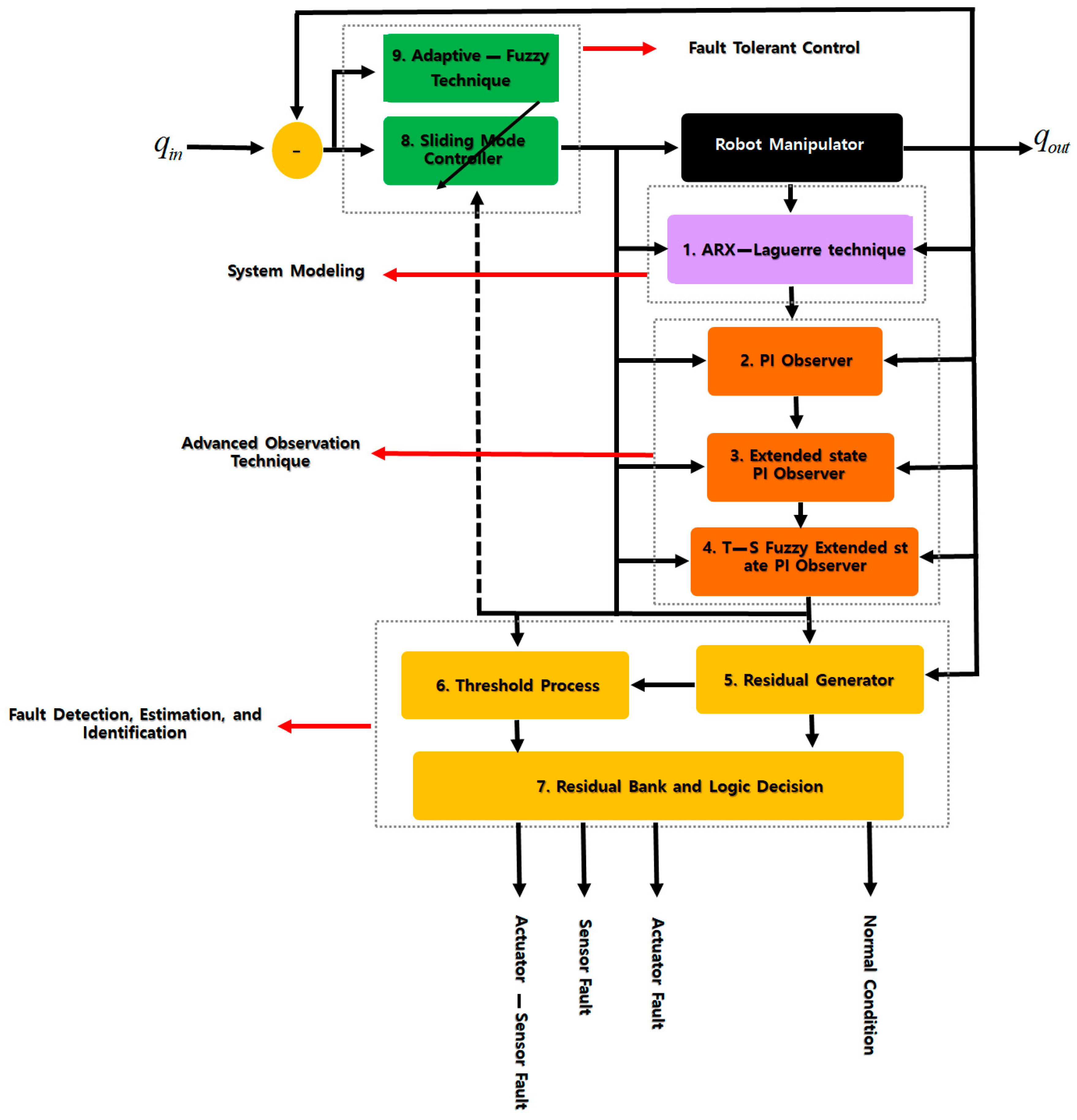
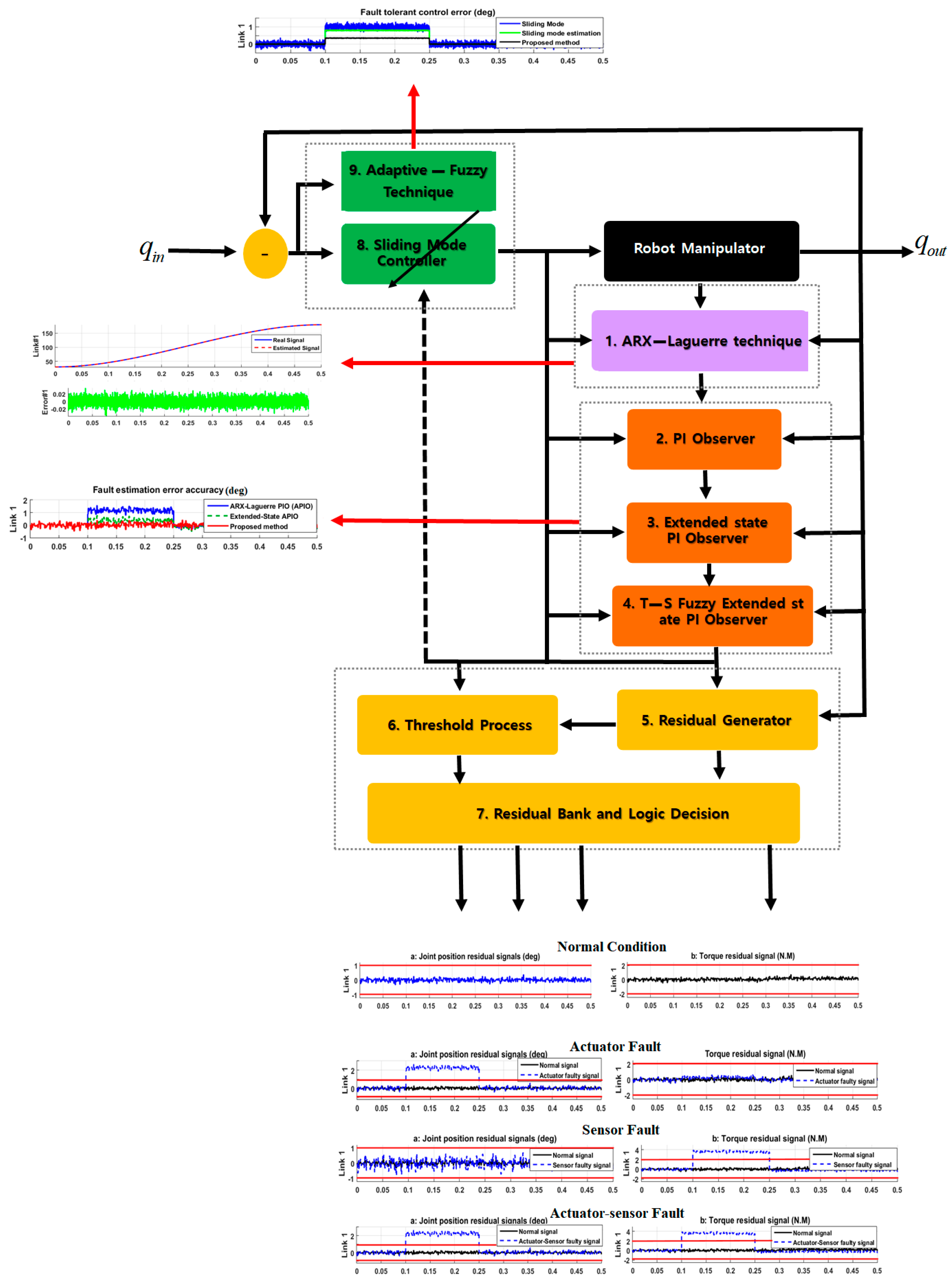
As shown in
Figure 1, the proposed adaptive sliding mode Takagi–Sugeno (T–S) fuzzy extended-state ARX–Laguerre PI observer consists of four main steps: (a) System modeling, (b) the advanced observation technique, (c) decision part for fault diagnosis, and (d) fault-tolerant algorithm. The ARX–Laguerre technique (block 1) is used for system modeling. The advanced observation algorithm is divided into three main steps: (a) The ARX–Laguerre PI observer, (b) sliding mode extended-state ARX–Laguerre PI observer, and (c) T–S fuzzy sliding mode extended-state ARX–Laguerre PI observer. The ARX–Laguerre PI observer (block 2) is used for system estimation based on the PI observation technique. While the ARX–Laguerre PI observer is easy to implement, the main drawback of this technique is robustness and fault estimation accuracy. To address the robustness issue, a sliding mode extended algorithm (block 3) is introduced. The sliding mode extended algorithm improves robustness, but chattering is the main drawback of this algorithm in an uncertain condition. To improve the fault estimation accuracy, a T–S fuzzy algorithm (block 4) is used. The fuzzy algorithm was designed using the PI technique to reduce fault estimation error. The decision part has three main units: (a) Residual generation, (b) threshold generation, and (c) residual bank and logic decision. In the residual generation part (block 5), the residual signals in different conditions are calculated. The threshold unit (block 6) is used to find the best threshold value for fault detection and identification. Based on blocks 5 and 6, the residual bank and logic decision (block 7) is used for fault detection and identification. After fault diagnosis, the fault-tolerant control is designed using the following three steps: (a) Sliding mode control algorithm, (b) observer-estimation technique, and (c) fuzzy adaptive algorithm. The sliding mode control algorithm (block 8) is a robust and stable technique in certain and uncertain conditions. To increase the performance of this algorithm in an uncertain condition, the observation estimation (block 8) is used. The proposed T–S fuzzy extended ARX–Laguerre PI observer is used to improve fault estimation accuracy for the sliding mode fault-tolerant algorithm. To solve the chattering problem in a faulty condition, a fuzzy-based algorithm is used for online tuning of the sliding surface slope coefficient in the proposed observer estimation sliding mode technique (block 9). The proposed approach of this paper makes the following contributions: (a) It increases the robustness of the ARX–Laguerre PI observer by using a sliding mode extended algorithm, (b) reduces chattering and improves the accuracy of fault modeling (estimation) for the extended-state ARX–Laguerre PI observer by using the T–S fuzzy technique, (c) reduces the fault effect in the T–S fuzzy extended ARX–Laguerre PI observer by using the classical sliding mode fault-tolerant control, (d) increases the performance of classical sliding mode controller in unlimited uncertain (faulty) condition by using the proposed T–S fuzzy extended-state ARX–Laguerre PI observer, and (e) tunes the sliding surface (switching gain) for chattering attenuation in the observer estimation sliding mode fault-tolerant control by using the fuzzy adaptive technique.
The rest of this paper is organized as follows. In
Section 2, the robot manipulator is modeled using the ARX–Laguerre procedure. The proposed robust adaptive fuzzy sliding mode extended ARX–Laguerre PI observer for robot manipulator fault detection, estimation, identification, and tolerant control is presented in
Section 3. In the first step of that process, a PI observer is built using the ARX–Laguerre technique; in the second step, the extended-state sliding mode algorithm is added to the ARX–Laguerre PI observer to improve its reliability and robustness; in the third step, a T–S fuzzy–based estimator is applied to the robust ARX–Laguerre extended-state PI observer to improve its estimation accuracy and convergence. In
Section 4, a sliding mode control technique is designed for fault-tolerant control. To improve the fault-tolerant control algorithm and reduce the chattering, an adaptive fuzzy algorithm is applied to the sliding mode technique. In
Section 5, the fault detection, estimation, identification, and tolerant control of the proposed algorithm are analyzed using a programmable universal manipulation arm (PUMA) robot manipulator. Conclusions are provided in
Section 6.
2. Robot Manipulator Modeling
A PUMA robot manipulator is a six degrees of freedom (DOF), serial linked, highly nonlinear, time-varying, and strong coupling effects system. The dynamic formulation for a robot manipulator is described below [
1]:
where
and
are an
torque vector, time variant
inertial matrix, time variant velocity matrix, time variant
gravity vector, position vector, velocity vector, acceleration vector, and robot manipulator’s faults and uncertainties, respectively. Based on Equation (1), the joint position is introduced as follows [
1]:
Using Equations (1) and (2), the state–space equation for the robot manipulator is calculated [
10]:
where
. The robot manipulator’s dynamic behavior in a theoretical or practical application might vary, which increases the challenge of fault diagnosis and tolerant control. To address that issue, the ARX–Laguerre system estimation method is used. As shown in
Figure 1, block 1 shows the ARX–Laguerre technique for system modeling and estimation. The ARX–Laguerre method for robot manipulator modeling is defined as [
10]:
where
, and
are the output joint variable (position), the Fourier coefficients, robot manipulator’s order, Laguerre orthonormal functions, convolution product, input signal (torque), filter position output, and filter position input, respectively.
Using Equation (4), the state–space robot manipulator modeling based on the ARX–Laguerre technique is generated as follows:
where
, and
are the state–function of the robot manipulator, (state, output, and input) coefficients, position output, torque input, robot manipulator faults and uncertainties, and Fourier coefficient, respectively.
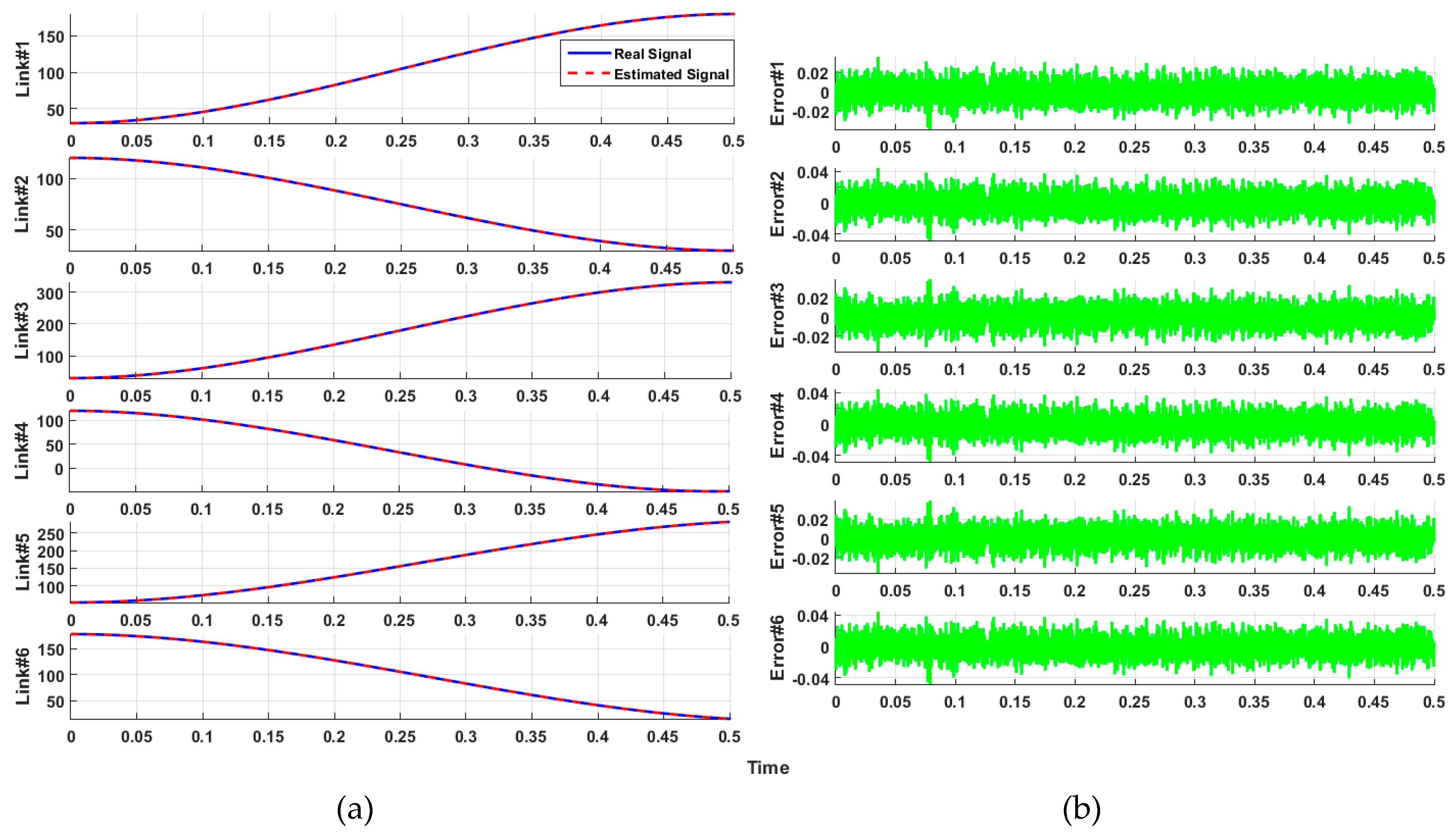
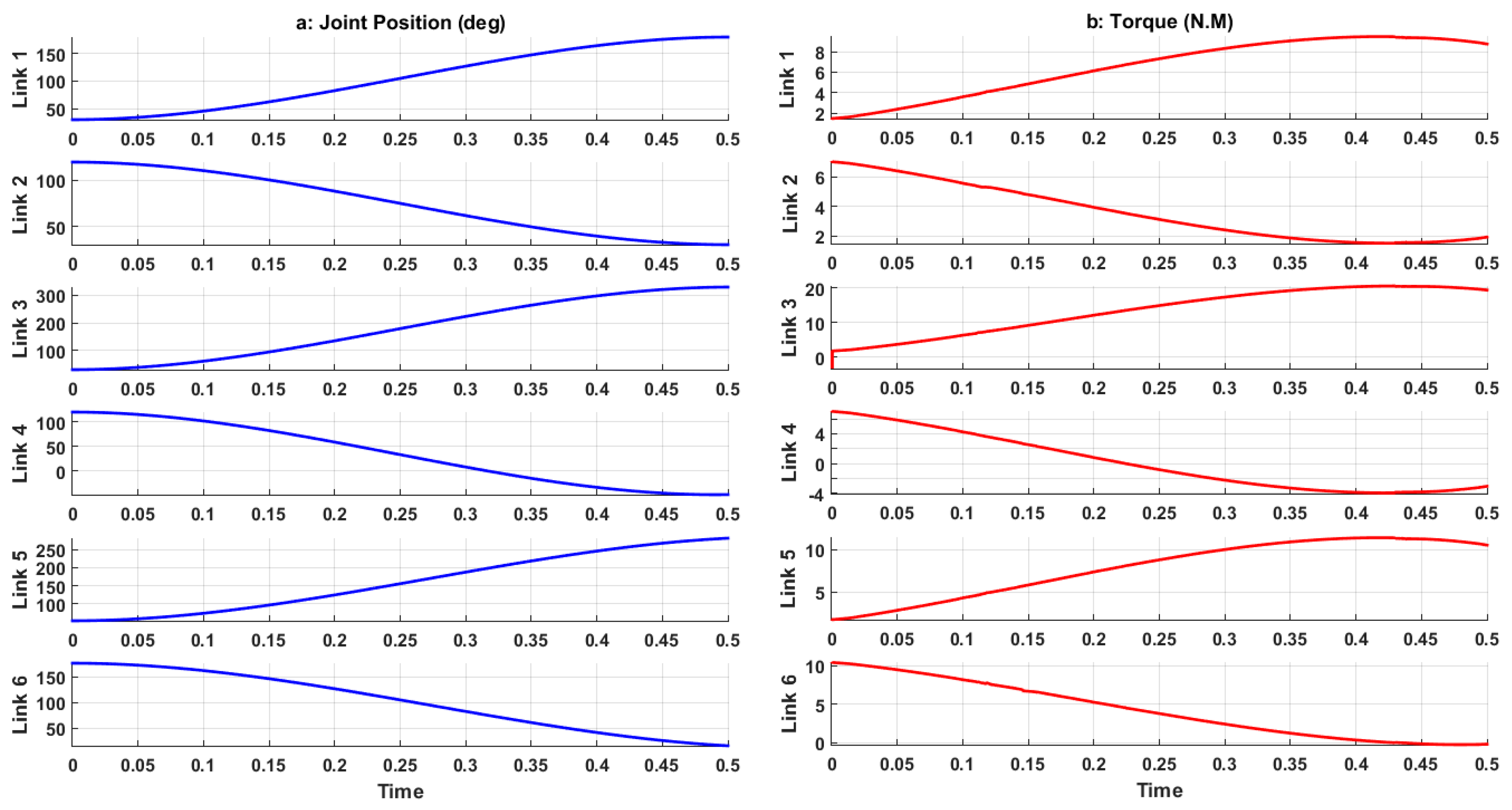
Figure 2 illustrates the estimation accuracy for the healthy condition based on the ARX–Laguerre technique. For the healthy state in
Figure 2, the sensitivity of the position estimation is exceptionally high, and the error rate is close to zero (less than 0.05°).
3. Proposed Method for Fault Estimation, Detection, and Identification
In
Figure 1, the proposed T–S fuzzy extended-state ARX–Laguerre PI observer for fault detection, estimation, and identification comprises six significant steps: ARX–Laguerre PI observer (block 2), sliding mode extended-state ARX–Laguerre PI observer (block 3) to improve the robustness of the ARX–Laguerre PI observer, estimation evaluator technique (block 4) that uses the T–S fuzzy technique to improve the fault estimation accuracy and reduce the chattering in the extended-state ARX–Laguerre PI observer, residual signal generator (block 5), threshold value calculation (block 6) based on the sliding mode algorithm, and fault detection and identification decision unit (block 7). Using the robot manipulator estimation based on the ARX–Laguerre technique presented in the previous Section, the ARX–Laguerre PI observer, block 2, for the robot manipulator is proposed as follows:
where
, and
are the PI observation-based state function, the PI observation-based position output, the PI observation-based faults and uncertainties estimation, and the PI observer (proportional and integral) coefficients, respectively.
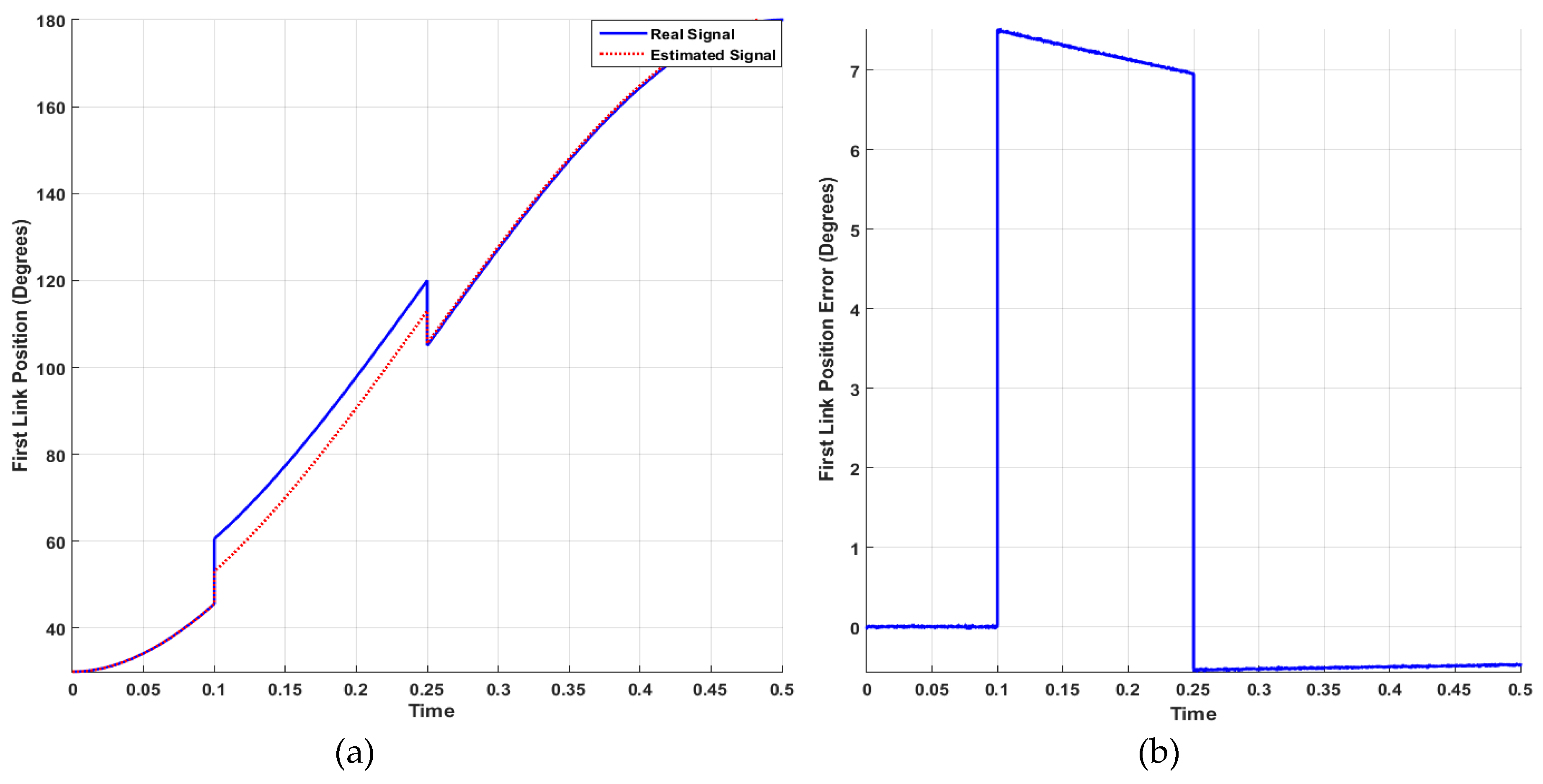
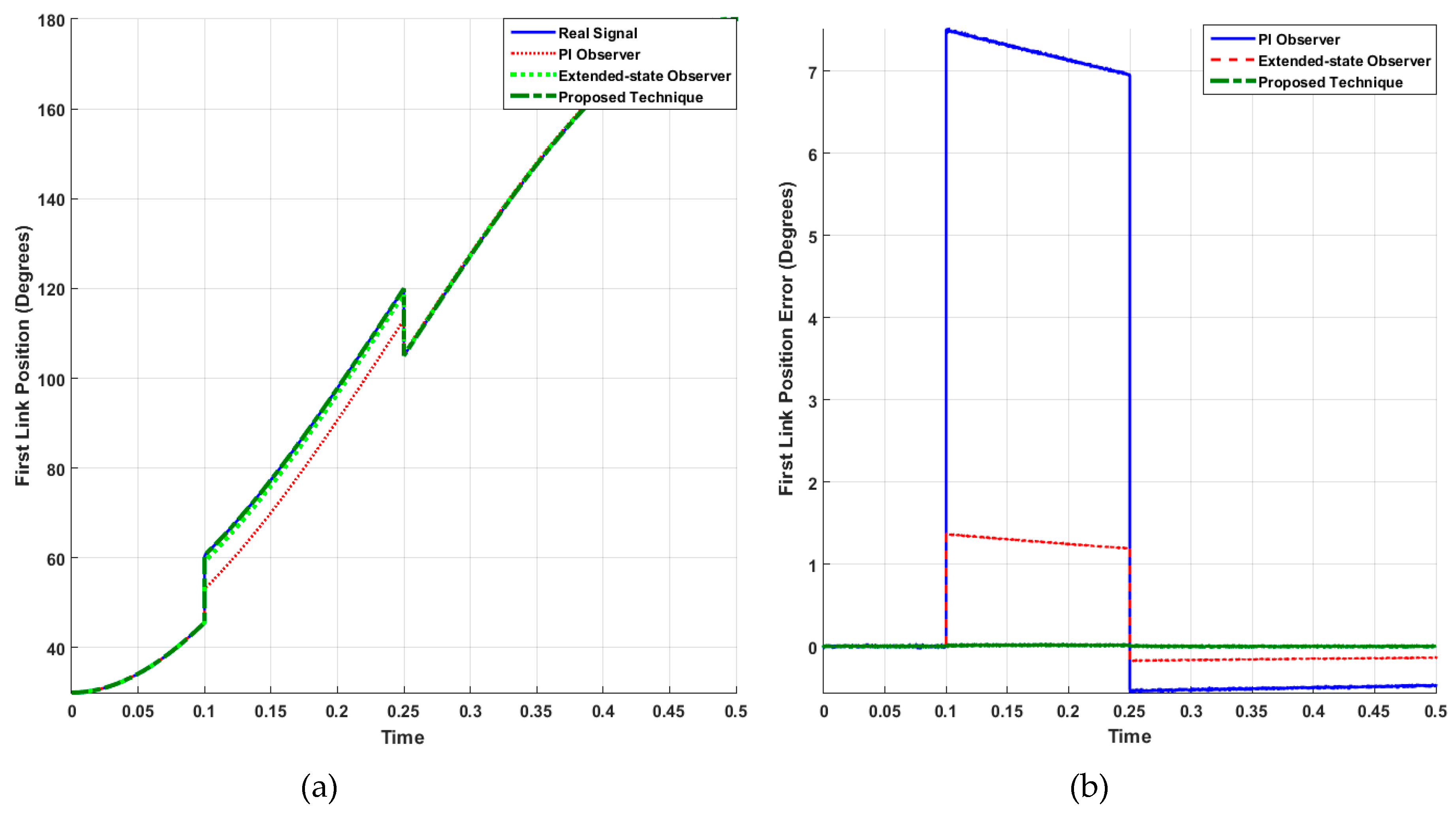
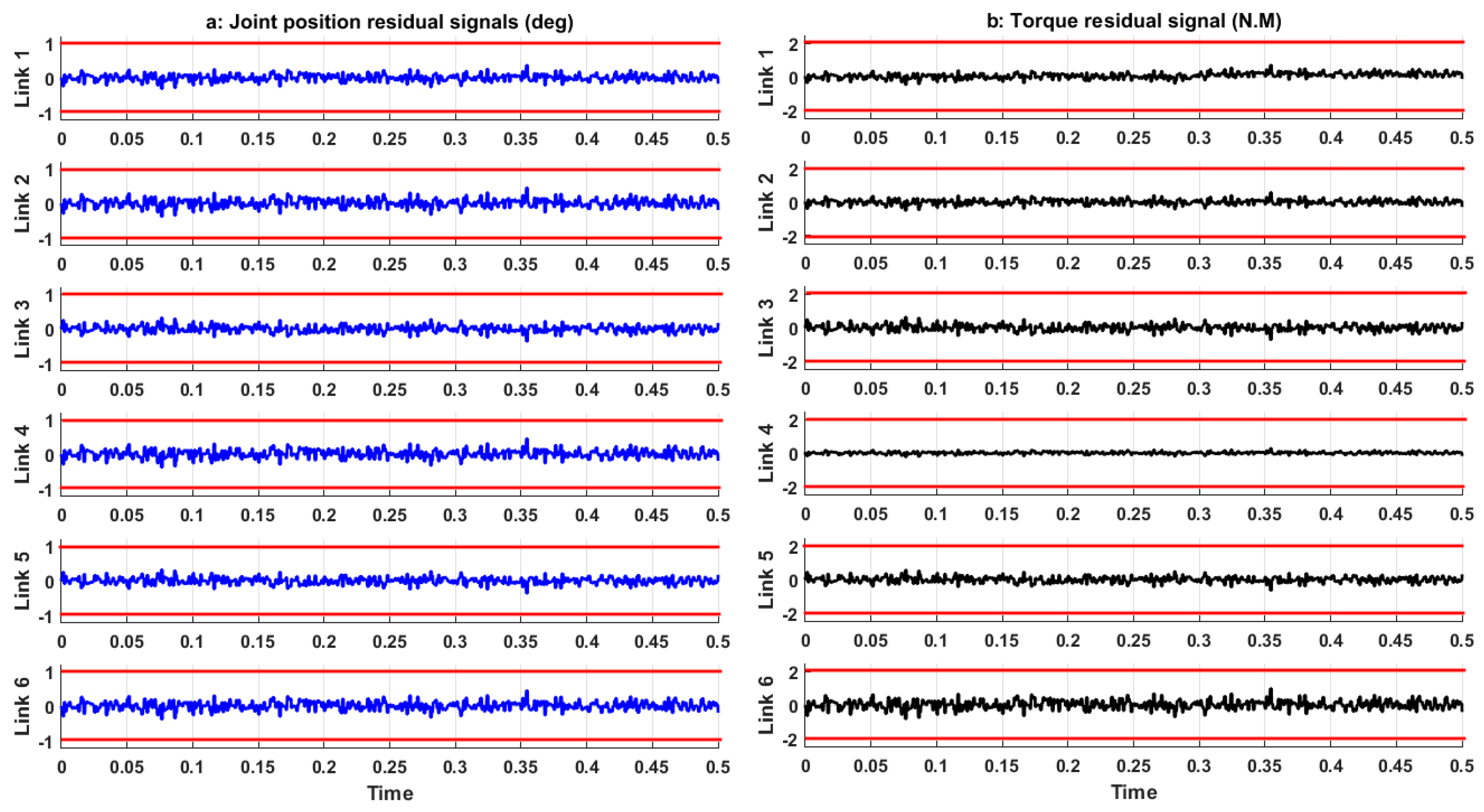
Figure 3 illustrates the effectiveness of the PI observer for fault estimation in the first link of the robot manipulator. As shown in
Figure 3, the error in the faulty signal estimation of the PI observer is not good enough for accurate fault estimation and identification.
In the next step, an extended-state sliding mode algorithm is used to modify the fault estimation, reliability, and robustness of the ARX–Laguerre PI observer, as represented in the following equation:
where
, and
are sliding mode extended observation-based state estimation, the sliding mode extended observation-based position output, the sliding mode extended observation-based faults and uncertainties estimation, the sliding mode faults and uncertainties estimation technique, and the sliding mode extended observation-based coefficients, respectively.
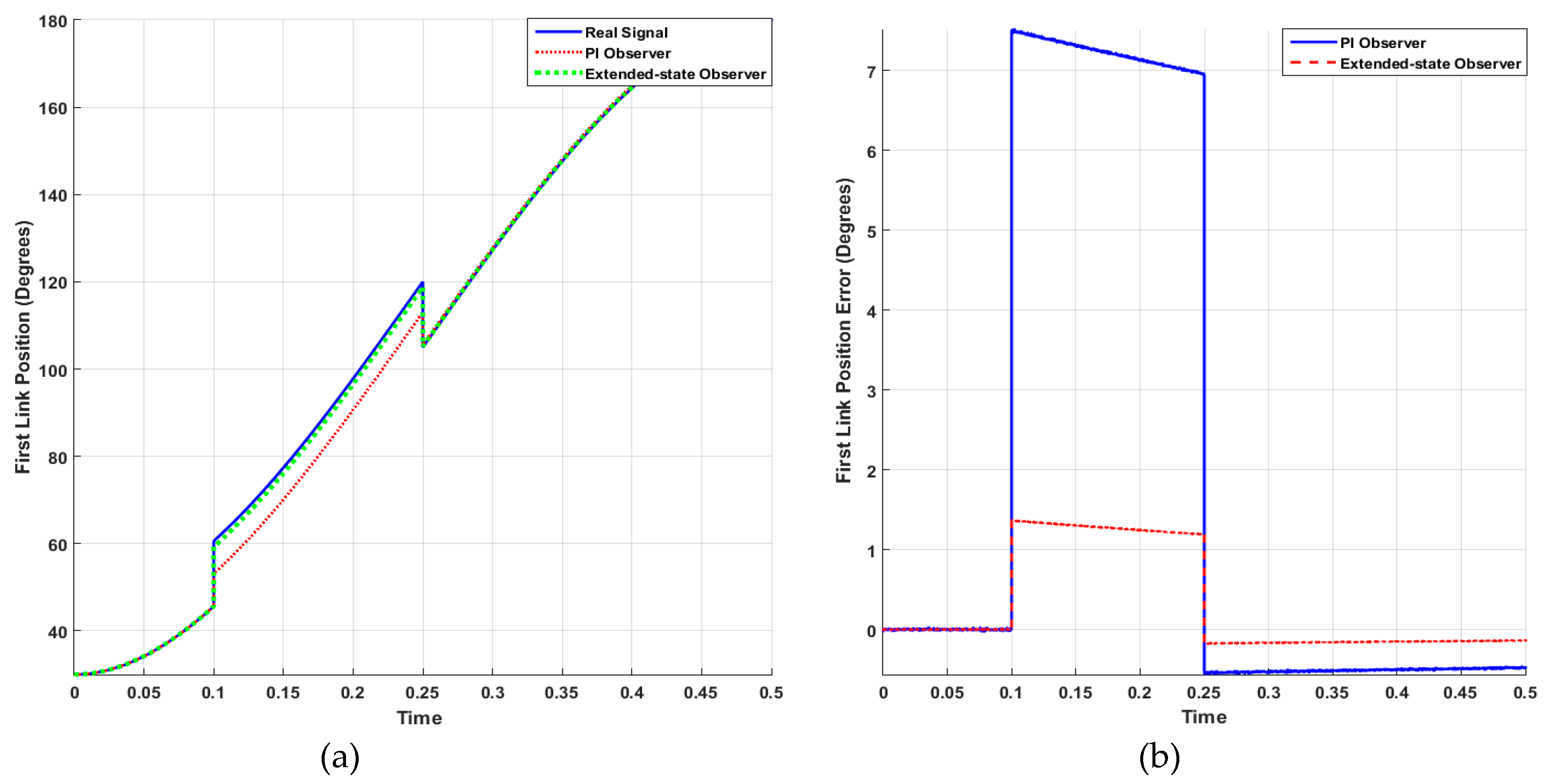
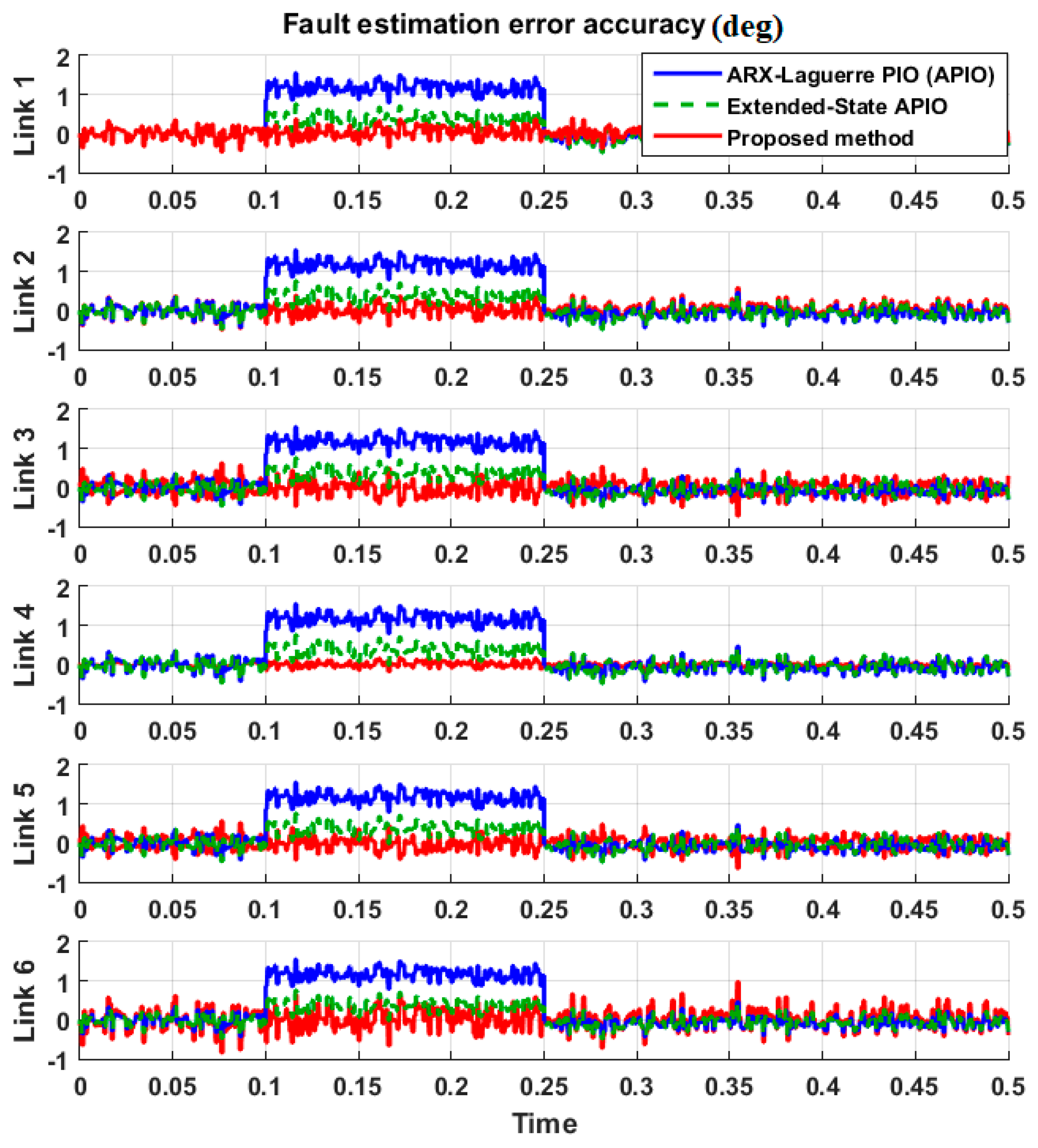
Figure 4 demonstrates the fault estimation efficiency of the sliding mode extended-state ARX–Laguerre PI observer for the first link of the robot manipulator error and improves the convergence of fault estimation. The T–S fuzzy definition is represented as follows [
15]:
where
, and
are the residual signal for the actuator fault, residual signal for the sensor fault, threshold values for the actuator and sensor faults, T–S fuzzy faults and uncertainties estimation signal, and fuzzy coefficient, respectively. The proposed T–S fuzzy algorithm for fault estimation is represented as follows:
where
and
are fuzzy logic coefficients for three different conditions (actuator fault, sensor fault, and actuator-sensor fault), actuator threshold, and sensor threshold, respectively:
As shown in
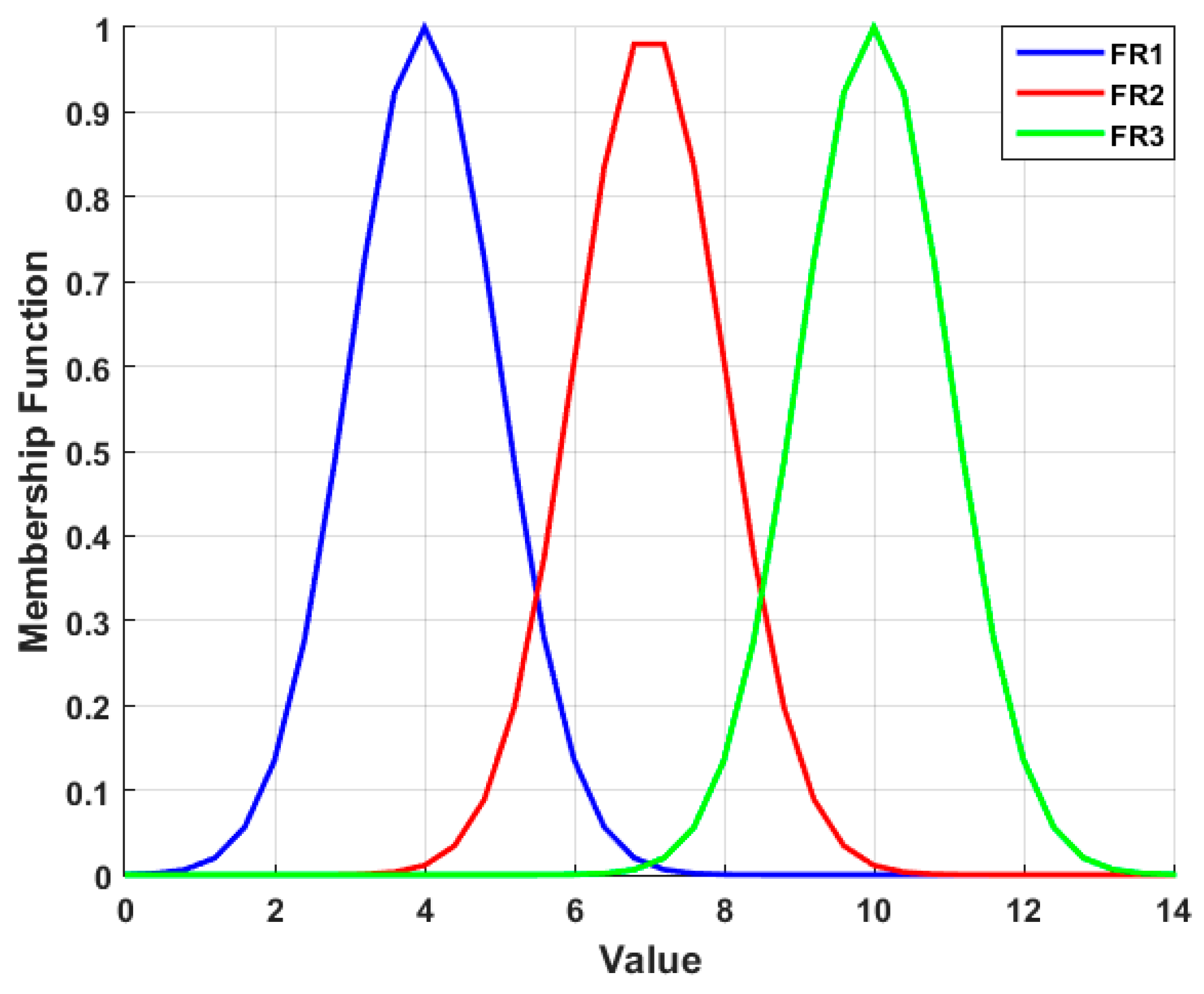
Figure 4, the performance of the extended-state ARX–Laguerre PI observer is more robust than that of the original ARX–Laguerre PI observer with a lower estimation error. After improving the signal estimation, reliability, and robustness of ARX–Laguerre PI observer via the sliding mode extended-state algorithm, the next block enhances the flexibility and accuracy of the fault estimation in an unknown condition. The T–S fuzzy algorithm is a powerful tool to reduce the error and improve the convergence of fault estimation. Three different membership functions are defined for T–S fuzzy fault estimation, as shown in
Figure 5. Therefore, based on Equations (7) and (9), the T–S fuzzy sliding mode extended-state ARX–Laguerre PI observer is proposed by the following equations:
Here,
, and
are the proposed observation-based state estimation, observation-based position output, and observation-based faults and uncertainties estimation, respectively. Therefore, the faults and uncertainties estimation signal
has three main parts: Integral term, sliding mode term, and fuzzy logic part.
Figure 6 illustrates the power of fault estimation based on the proposed T–S fuzzy extended-state ARX–Laguerre PI observer. As shown in
Figure 6, the error rate in the faulty signal estimation of the proposed T–S fuzzy extended-state ARX–Laguerre PI observer is lower than in the previous iterations (
Figure 3 and
Figure 4). Therefore,
is represented by Equation (10). After procurement the stability, the state space estimation of
converges to
, the estimation error converges to zero and
[
14]. The Lyapunov function of the proposed procedure is defined as follows:
The derivative of the Lyapunov is represented in Equation (12):
Here,
is the error of faults and uncertainty estimation. Based on Reference [
20], if
; thus,
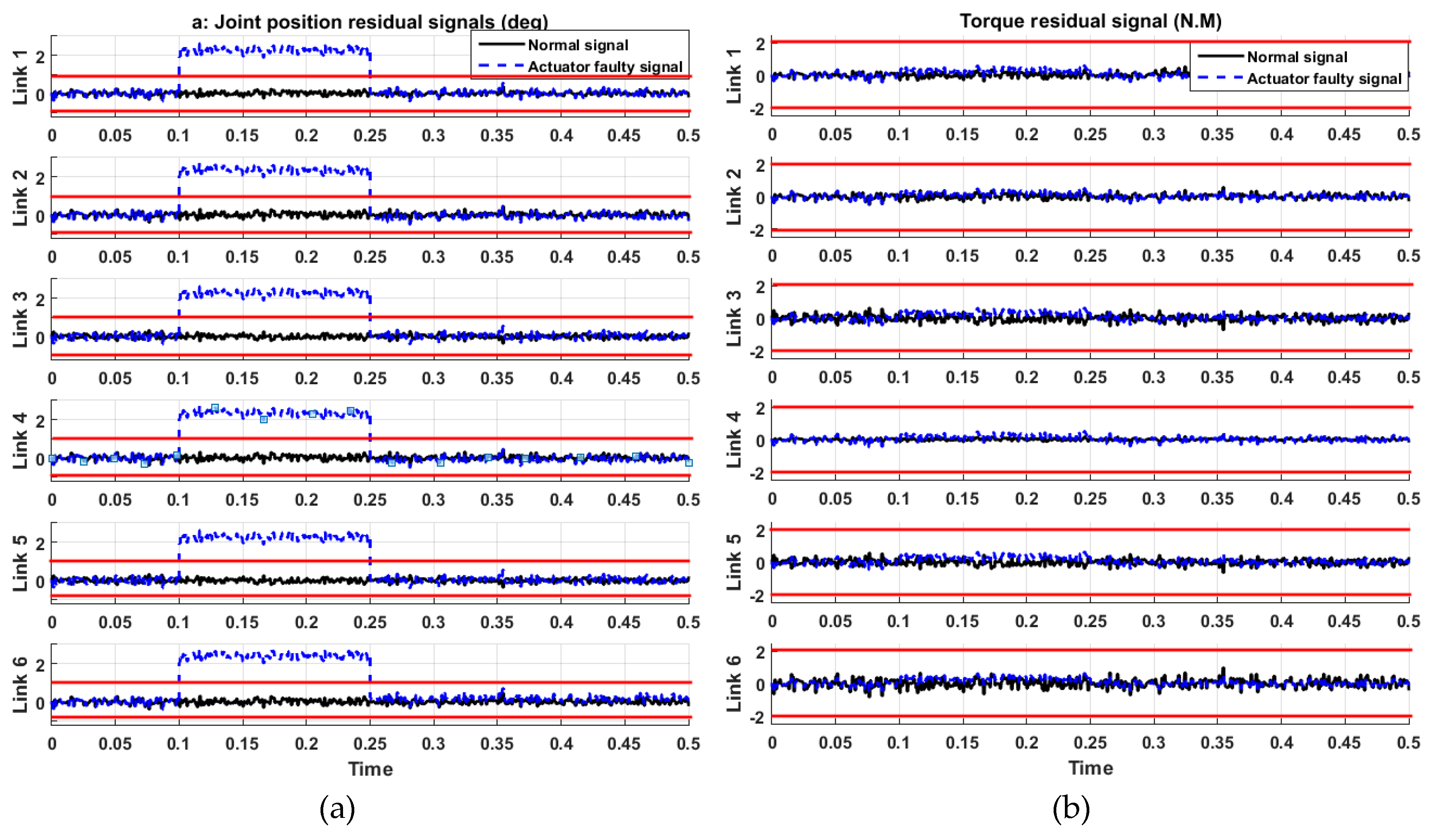
. Therefore, the fault estimation using the proposed algorithm can be converged to zero in the finite time. The residual signal is generated by the following equation:
The next step of the proposed algorithm is the threshold process. Various techniques have been used previously, but we employed the sliding mode algorithm [
10]. The following definition represents the threshold process based on the sliding-mode algorithm:
where
, and
are the actuator fault threshold value, sensor fault threshold value, coefficients of the sliding mode algorithm for threshold value calculation, actuator fault residual signal, and sensor fault residual signal, respectively.
The last block in
Figure 1 for fault detection, estimation, and identification is the logical decision. The main positive point in this study is an accurate fault estimation technique based on the T–S fuzzy sliding mode extended-state ARX–Laguerre PI observer. Based on Equation (10), the proposed faults and uncertainties estimation technique is represented by the following equation:
where:
As shown in
Figure 6, the error in the signal estimation with the proposed algorithm is close to zero. Based on Equations (13) and (14), the following algorithm is introduced for fault detection in the robot manipulator:
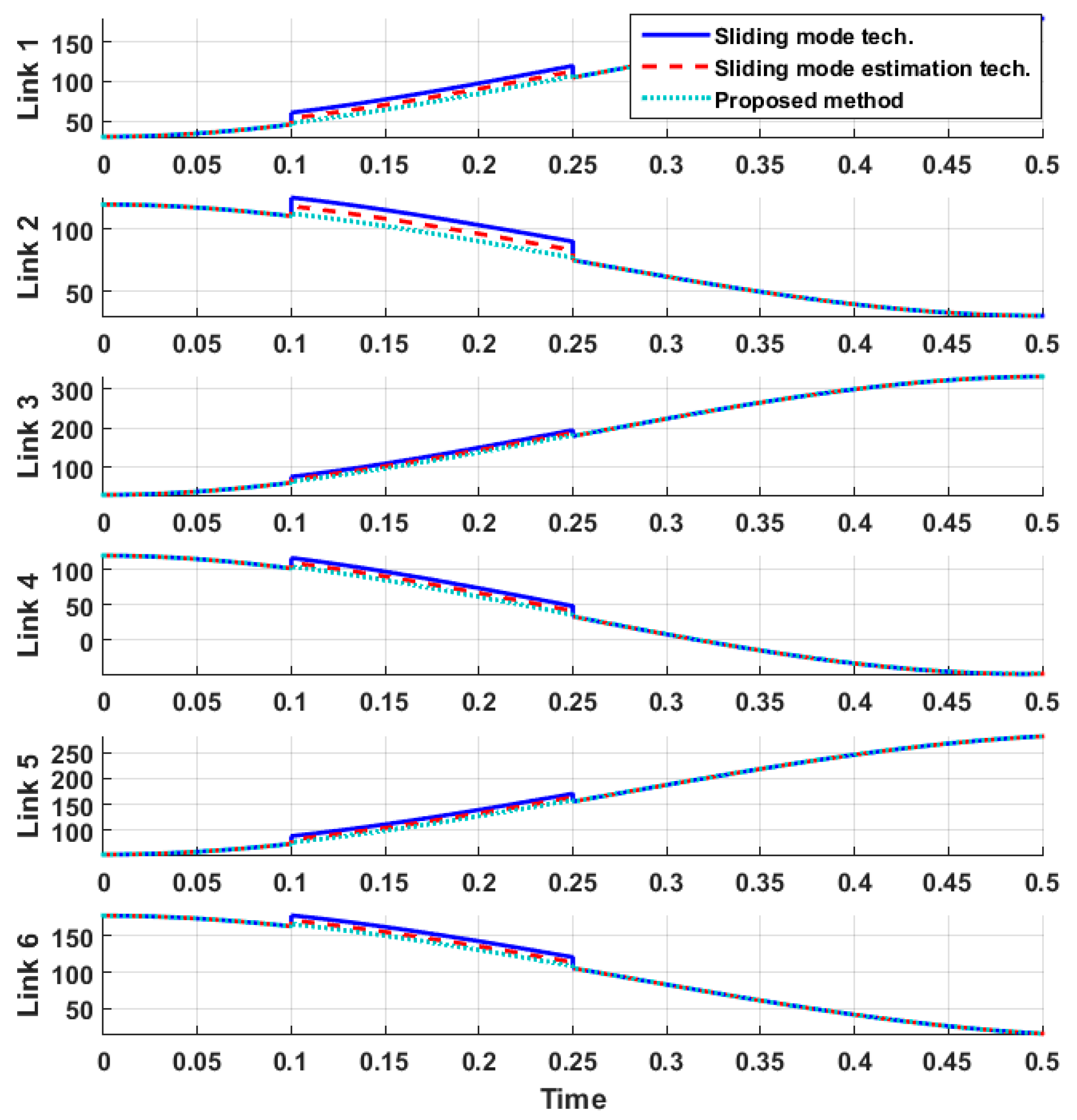
Fault identification is the third step in making a logical decision. In this research, we considered three types of faults: (a) Actuator faults, (b) sensor faults, and (c) actuator–sensor faults. To identify them, the following techniques are introduced:
The threshold value formulation is extracted from Equation (14). Sliding mode is a robust algorithm that can be used to design a robust controller and observer. In this study, we used this technique to calculate threshold values [
10]. In the first step, the residual signal is calculated based on Equation (13). In the second step, the sliding surface
is calculated to find the robust surface for each condition. We use an integral term of sliding surface to calculate the threshold value based on a steady-state residual signal. The residual signal and threshold values for various conditions (normal, actuator fault, sensor fault, and actuator–sensor fault) are completely different. In the third step, the switching function is used to find the maximum and minimum signal value
for each condition and improve the robustness. In the last step, threshold values are calculated. Thus, based on these threshold values, we can drive the decision logic part for fault detection and identification.
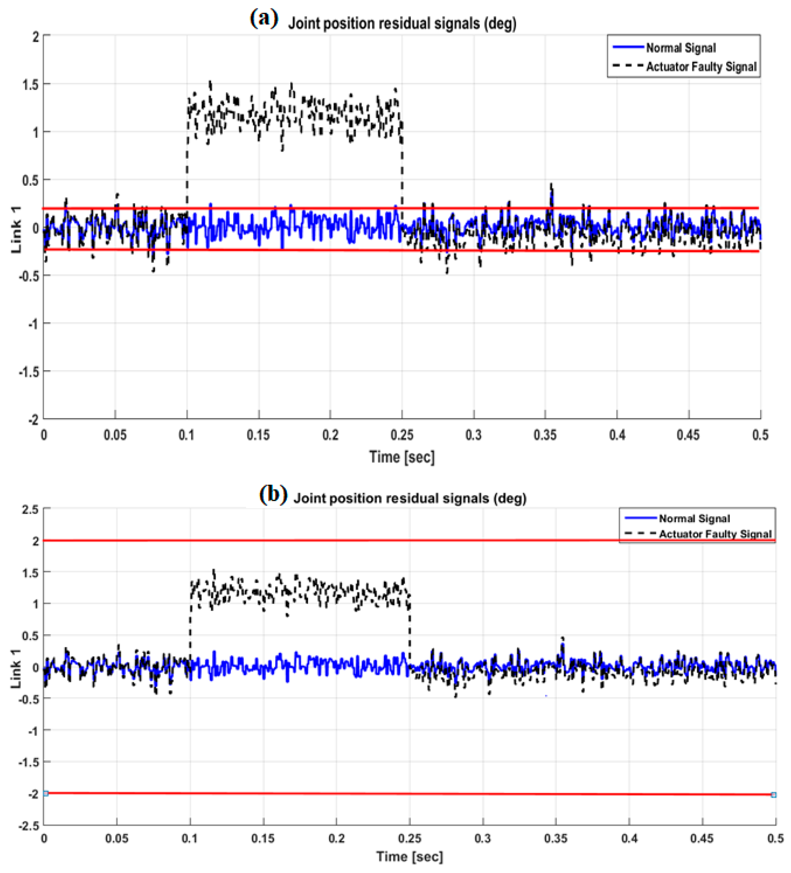
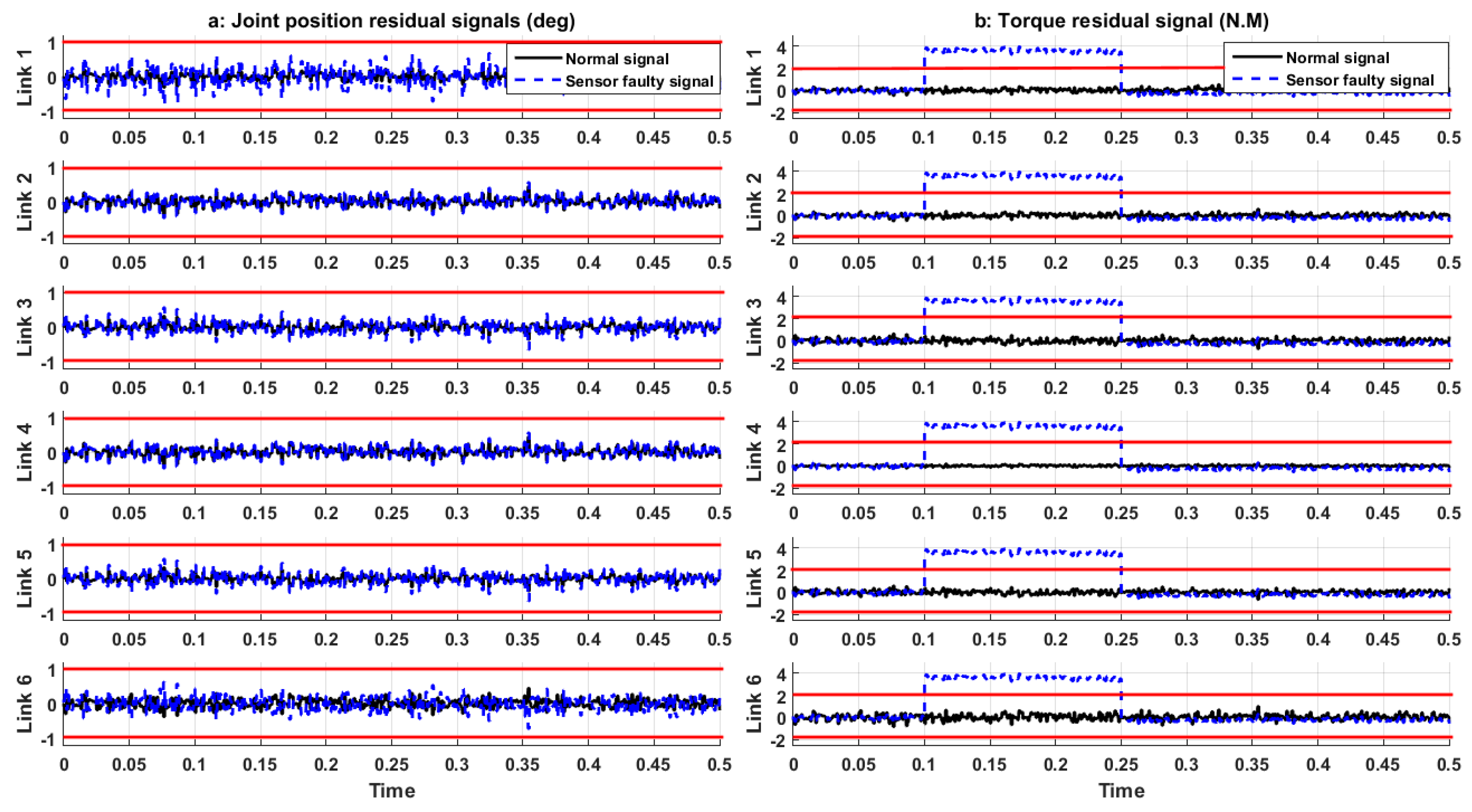
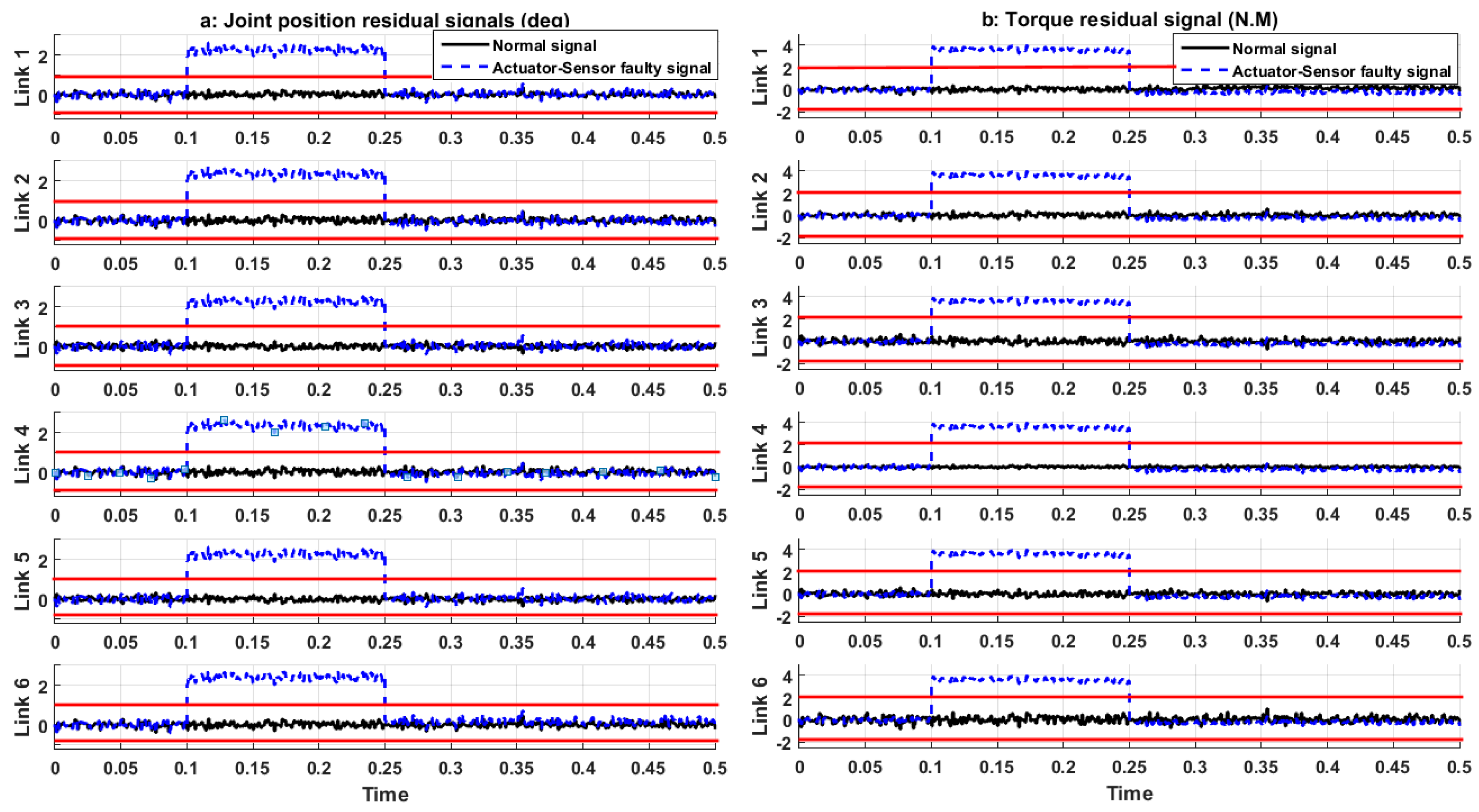
Figure 7 illustrates the effect of incorrect threshold values for fault detection in normal and actuator fault conditions. Based on
Figure 7a, the uncertainties and disturbances in normal condition are detected as faults and send an incorrect fault alarm to the fault-tolerant controller. In
Figure 7b, based on the threshold value, the proposed method cannot detect the faulty signal.
4. Proposed Method for Fault-Tolerant Control
In this Section, we describe the design for a robust, fault-tolerant controller. The fuzzy adaptive sliding mode controller with variable estimation is a robust fault-tolerant control algorithm. The first step is designing the sliding mode controller. The equation for conventional sliding mode fault-tolerant control is as follows [
16]:
where
, and
are the output signal of the sliding mode algorithm, the switching part of the sliding mode algorithm to compensate for unknown conditions, the model-equivalent part of the sliding mode control law, the desired state, the sliding surface, the derivative of the sliding surface, and the sliding slope coefficient, respectively. The Lyapunov function and the derivative of the Lyapunov function for conventional sliding mode fault-tolerant control are presented in Equations (20) and (21), respectively:
Here,
is a constant. As shown in Equations (20) and (21), if
,
, and the derivative of the Lyapunov function converges to zero in a finite time [
16].
Thus, the conventional sliding mode fault-tolerant control is robust and stable, but the chattering phenomenon and the system’s performance in faulty conditions remain problematic. Therefore, we introduce a sliding mode estimation fault-tolerant control. Its main positive point is that it can estimate the unmeasured variable
by observation. The formulation of the sliding mode estimation fault-tolerant control is represented as:
where
, and
are the output signal of the sliding mode estimation fault-tolerant algorithm, sliding surface slope in sliding mode estimation controller, and the observer estimation part, respectively. The Lyapunov and the derivation of Lyapunov function are defined by the following formulation:
If the normal threshold value with respect to the uncertainties and disturbances is defined by
for
, we have:
Based on Equation (28),
, and the derivative of the Lyapunov function converges to zero in a finite time [
16]. Based on Equations (25) and (26), the uncertainties and disturbances in normal and abnormal condition can be bounded by:
Here,
and
are the normal threshold value and the uncertainties in a normal condition. Based on Equations (19), (24), and (29),
, and thus,
, and the chattering generated by the sliding mode estimation fault-tolerant control is meaningfully reduced compared to the conventional sliding mode fault-tolerant control. To improve the performance of the sliding-mode estimation fault-tolerant control, a fuzzy adaptive technique is proposed. Since the fault varies with respect to various conditions and is difficult to predict, calculating the minimum switching gain
is very difficult. Increasing the value of the switching gain increases the chattering phenomenon. If the switching gain varies with the condition of the robot manipulator, chattering could be reduced. On the other hand, modeling a fault is very complicated; therefore, a fuzzy algorithm is designed for online tuning of the switching gain. Beginning from Equation (24), the adaptive fuzzy sliding mode estimation fault-tolerant control can be written as:
Here,
, and
are the output signal of the proposed fault-tolerant algorithm, the online tuning switching part of the proposed algorithm, and the auto-tuned sliding slope coefficient, respectively. The
is a coefficient determined by the designed fuzzy technique as follows:
The position output is designed as a fuzzy input, and the sliding surface is designed as the second input of the fuzzy algorithm. The fuzzy rule-base is defined as:
If the fuzzifier of the fuzzy set is a singleton, and the defuzzification technique is a center average, the fuzzy set is defined as:
where
, and
are the fuzzy inputs, fuzzy sets, and fuzzy output, respectively. Therefore, if the fault-tolerant controller is designed as shown in Equation (24) with the adaptive gain tuning technique given in Equation (30) and the online switching gains as determined in Equation (33), the fault-tolerant controller is stable [
21]. For the first fuzzy input
in the interval
, the fuzzy membership functions are designed based on the Gaussian type, and the fuzzy sets are defined as negative big (NB), negative medium (NM), negative small (NS), zero (Z), positive small (PS), positive medium (PM), and positive big (PB). For the second fuzzy input
in the interval
, the fuzzy membership functions are designed based on the Gaussian type, and the fuzzy sets are again NB, NM, NS, Z, PS, PM, and PB. For the fuzzy output
in the interval
, the fuzzy membership functions are designed based on the Gaussian type and the fuzzy sets are PS, PM, and PB. The fuzzy rule table is given in
Table 1.
Algorithm 1 illustrates the adaptive T–S fuzzy sliding mode extended-state ARX–Laguerre PI observer for fault detection, estimation, identification, and tolerant control of a robot manipulator.
Figure 8 illustrates the proposed method as a block diagram for fault diagnosis and fault-tolerant control.
6. Conclusions
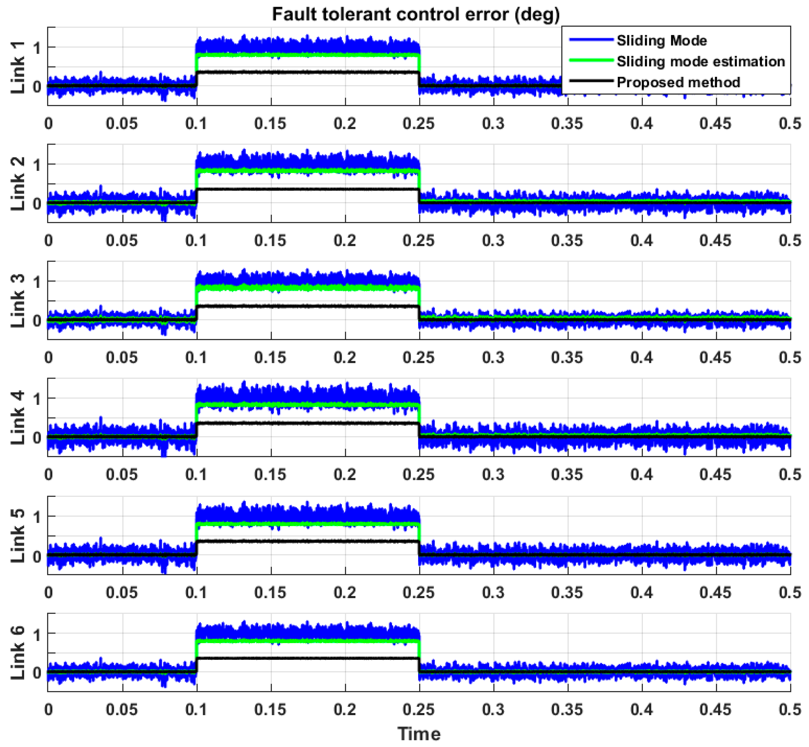
This paper explored fault detection, estimation, identification, and tolerant control using the proposed adaptive fuzzy sliding mode estimation extended-state ARX–Laguerre PI observer algorithm for a robot manipulator. First, the system’s dynamic was modeled and estimated based on the robust ARX–Laguerre technique. Second, for fault detection, estimation, and identification, an ARX–Laguerre PI observer was designed. To improve the reliability, robustness, and signal estimation of the ARX–Laguerre PI observer, the third step considered a sliding mode extended-state observer. Despite enhancing the robustness and reliability of the method, the accuracy of its faulty signal estimation still needed to be improved. Therefore, in the fourth step, the T–S fuzzy algorithm was used to improve the estimation accuracy of the sliding mode extended-state ARX–Laguerre PI observer. As shown in the results, the proposed algorithm is a reliable technique for fault detection, estimation, and identification. Because of its reliability and robustness, the sliding mode algorithm technique was introduced as the main algorithm for fault-tolerant control of a robot manipulator. To improve the power of fault attenuation, the estimated fault calculated by the proposed T–S fuzzy sliding mode extended-state observer in the previous step was applied to the classical sliding mode technique. As demonstrated in the results, the power of fault attenuation in the sliding mode estimation algorithm was better than that in the conventional sliding mode algorithm. In addition, the fuzzy adaptive sliding mode estimation fault-tolerant control algorithm was designed to reduce chattering and improve fault attenuation. The effectiveness of the proposed algorithm for fault diagnosis and fault-tolerant control was tested using a PUMA robot manipulator. The results and analysis demonstrated that the proposed algorithm estimates and identifies defects and attenuates the defects and chattering in the presence of uncertainty and disturbance. In the future, a higher-order intelligent extended-state sliding mode controller-observer will be designed for fault estimation-based fault diagnosis and tolerant control.


