Estimating Adaptive Setpoint Temperatures Using Weather Stations

 ,
,  ,
,  and
and
Abstract
:1. Introduction
1.1. Energy Consumption of Residential Buildings
1.2. Adaptive Setpoint Temperatures
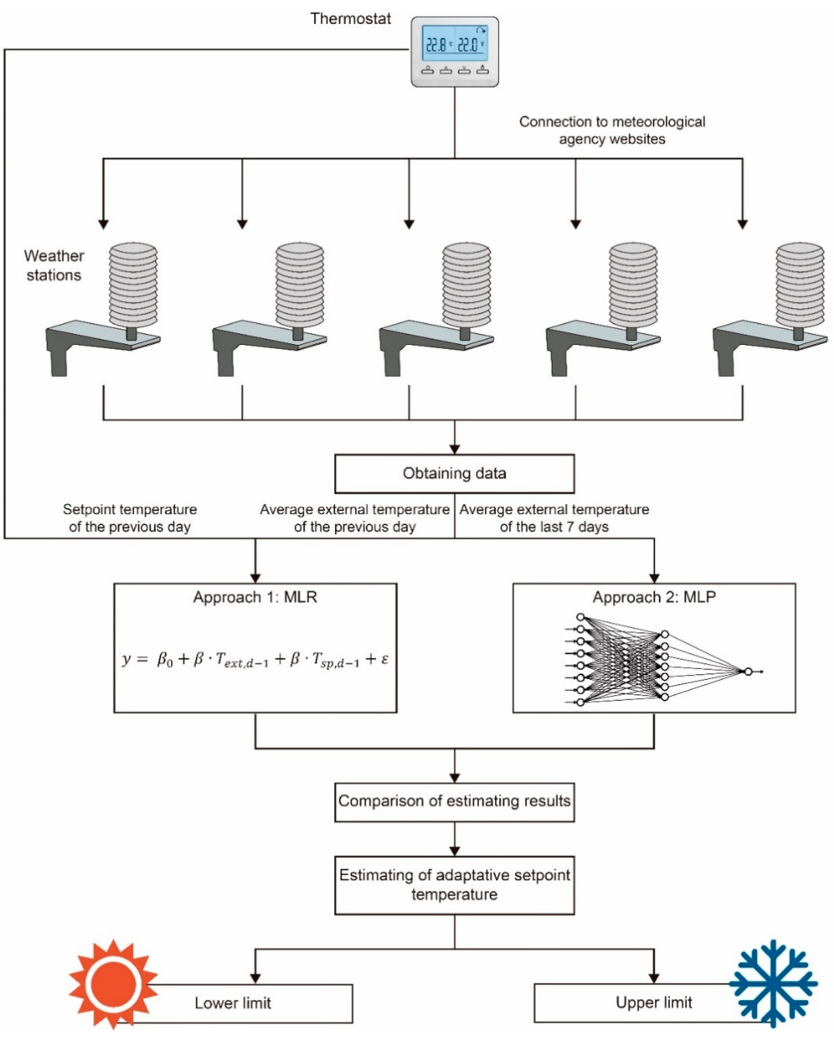
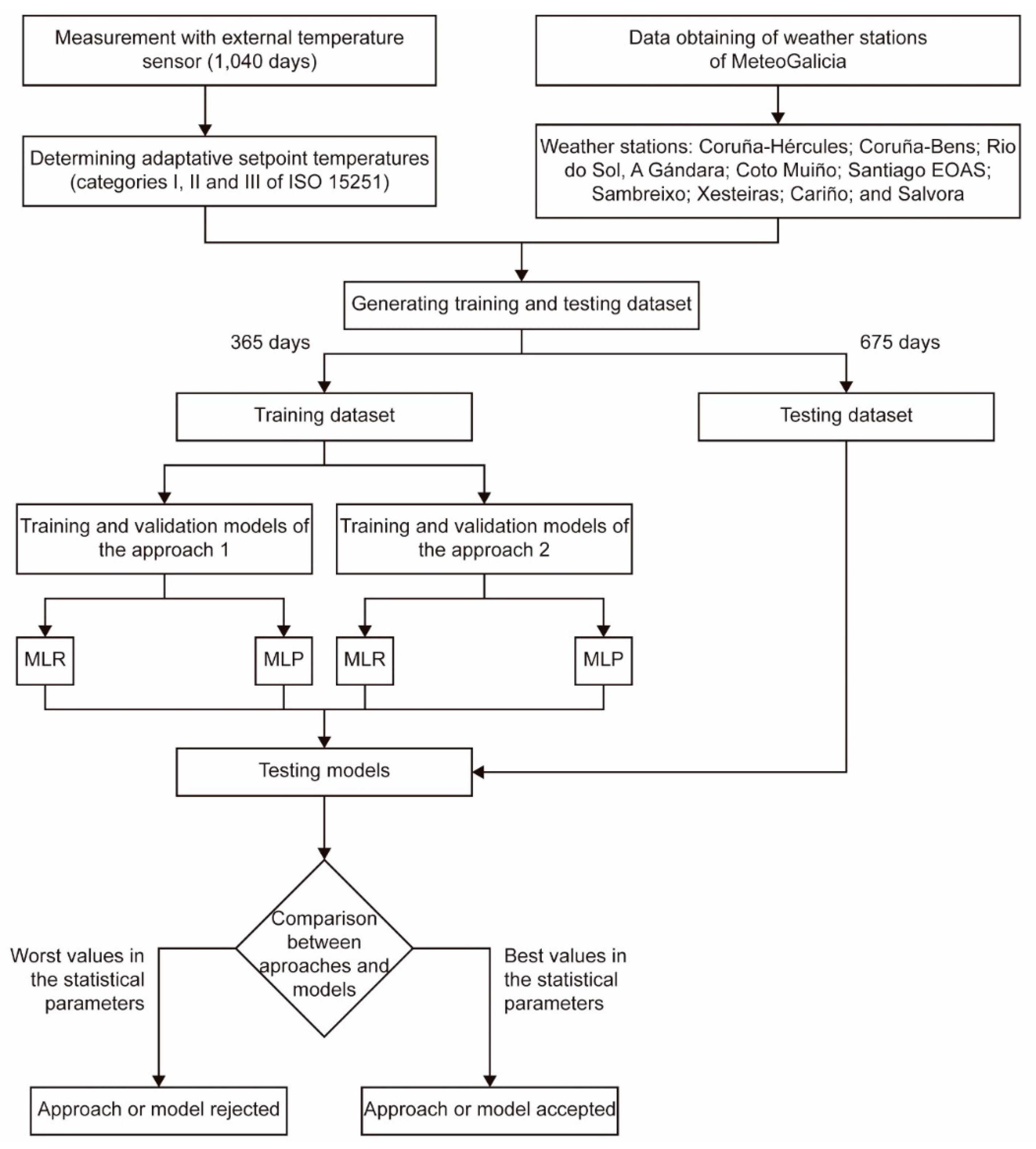
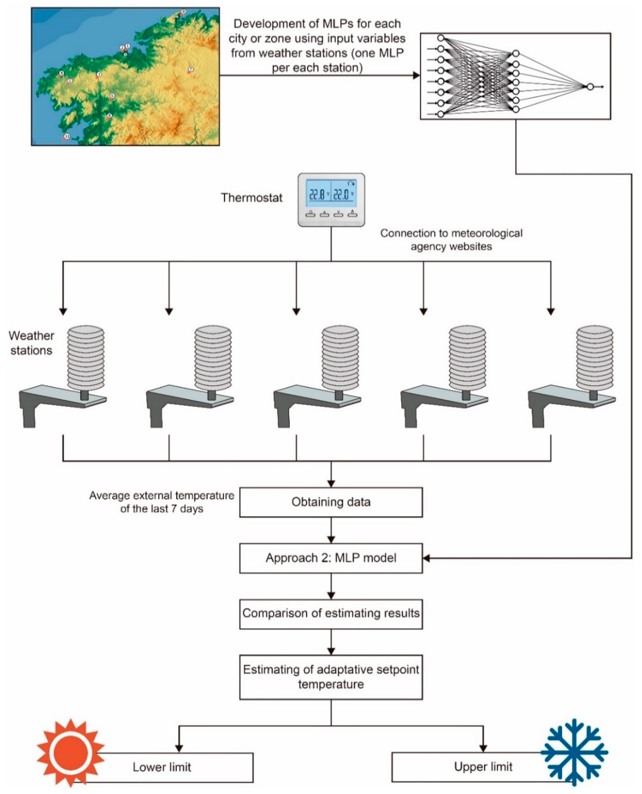
2. Methodology
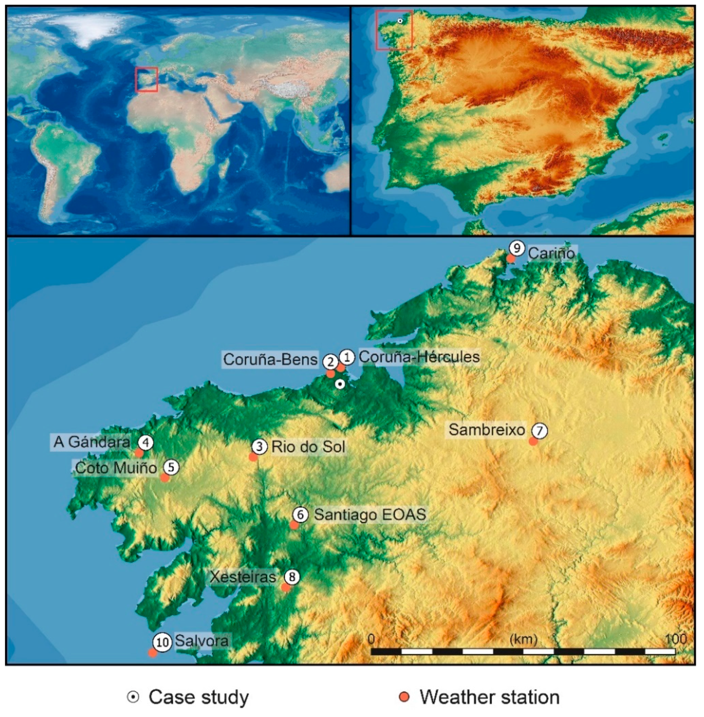
2.1. Case Study
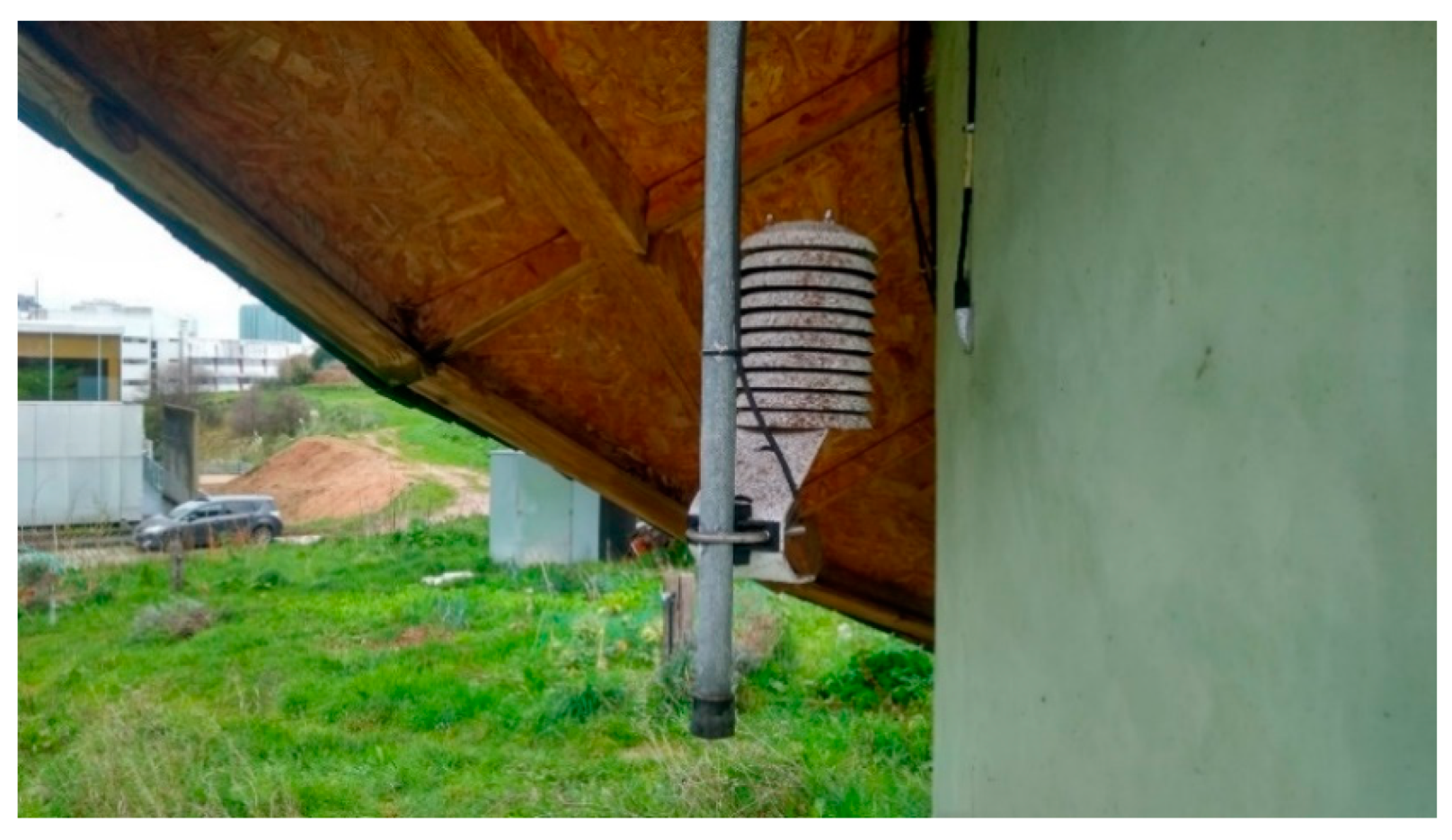
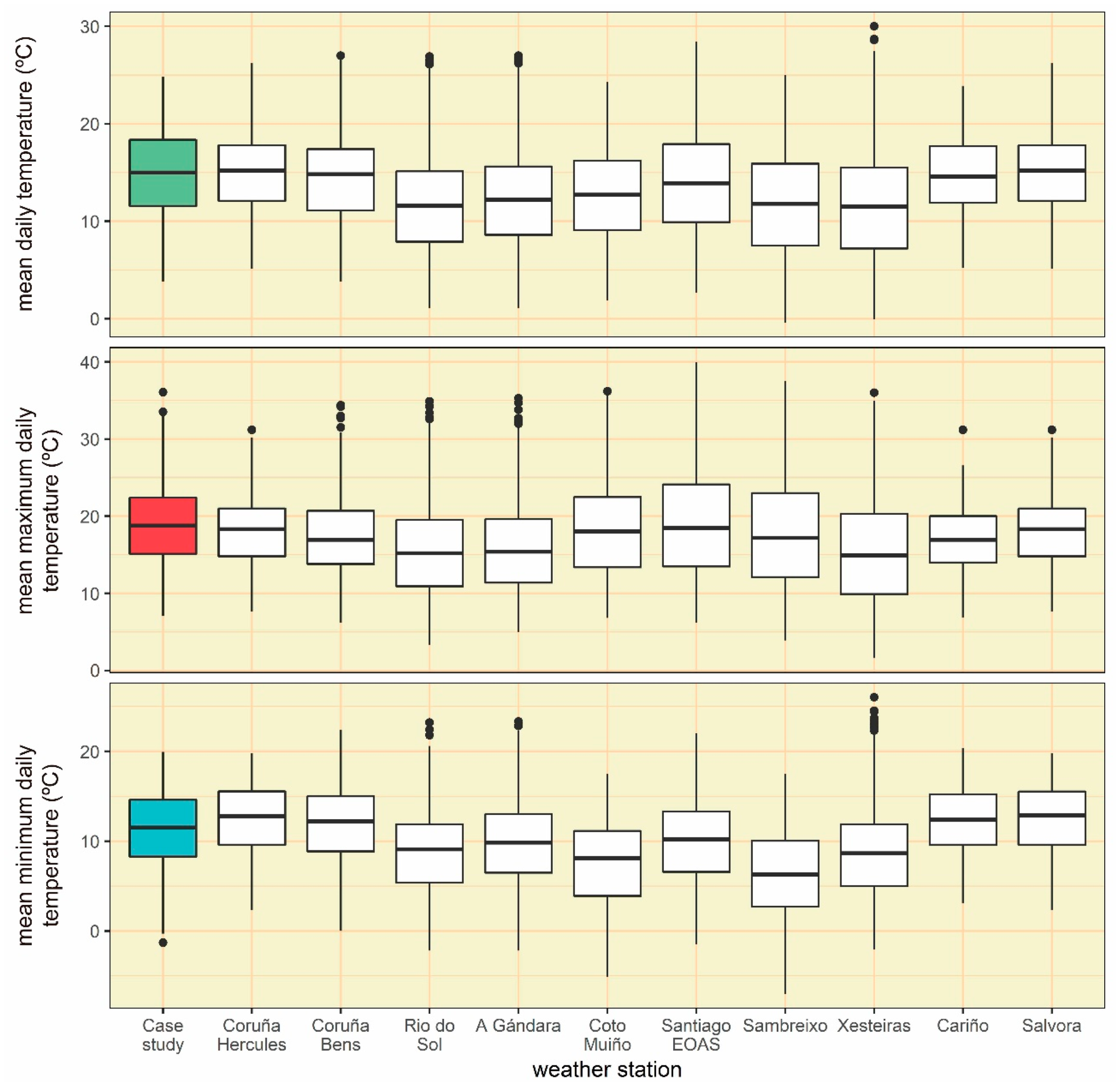
2.2. Weather Stations
2.3. Approaches for Estimating Adaptive Setpoint Temperatures
2.4. The Regression Algorithms Used
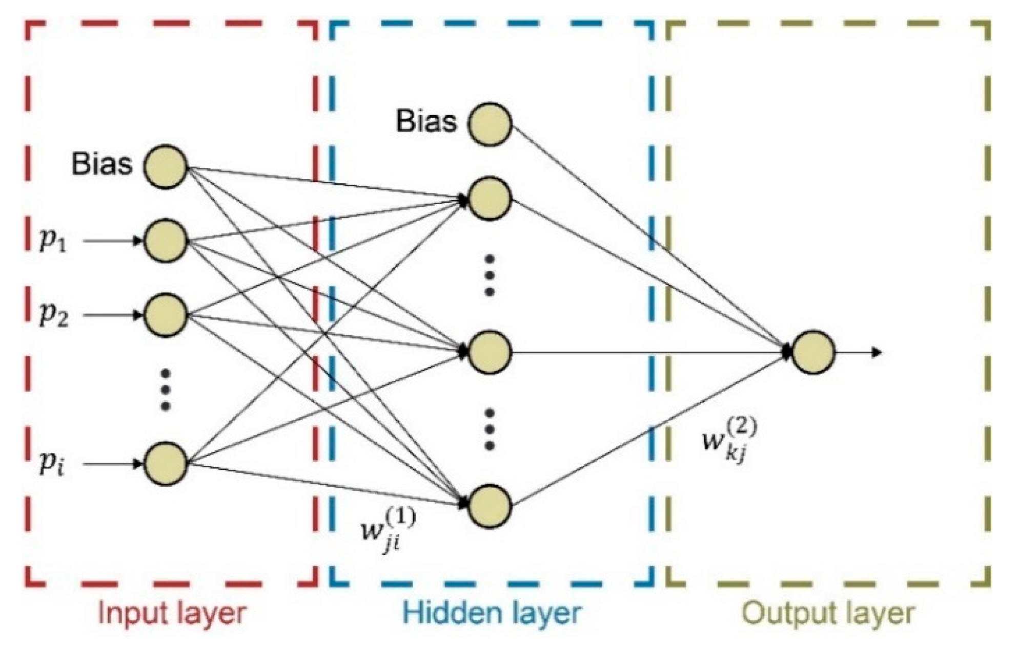
2.4.1. MLR
2.4.2. MLP
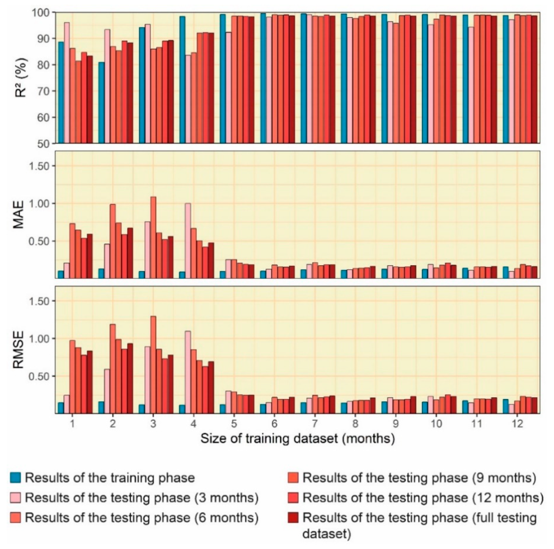
2.5. Dataset, Training, and Testing of the Models
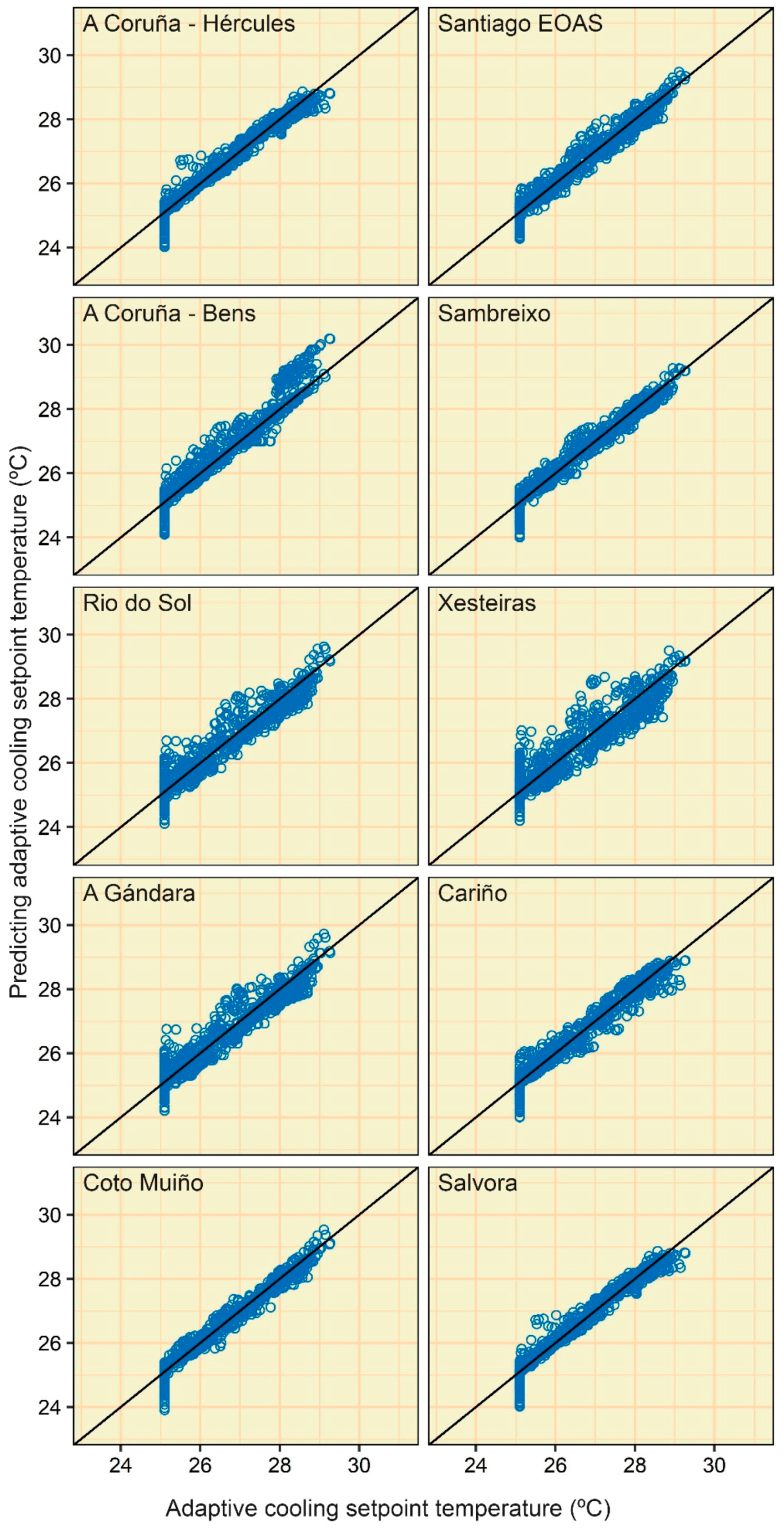
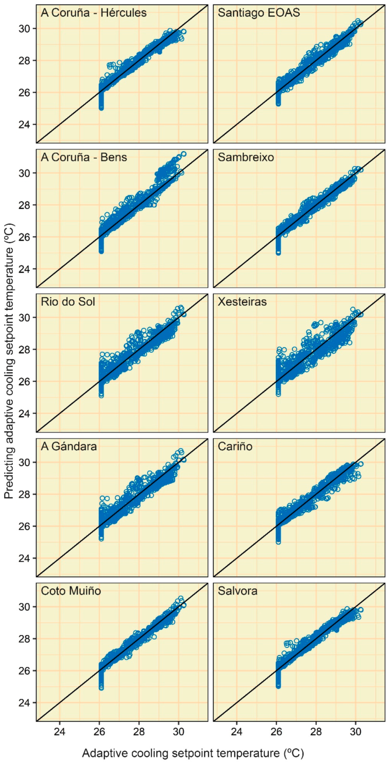
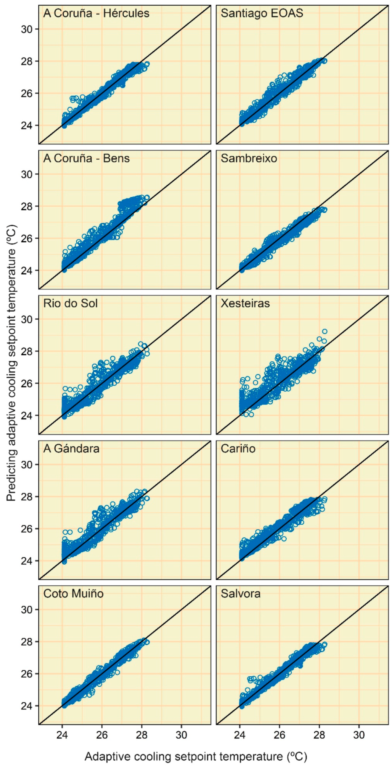
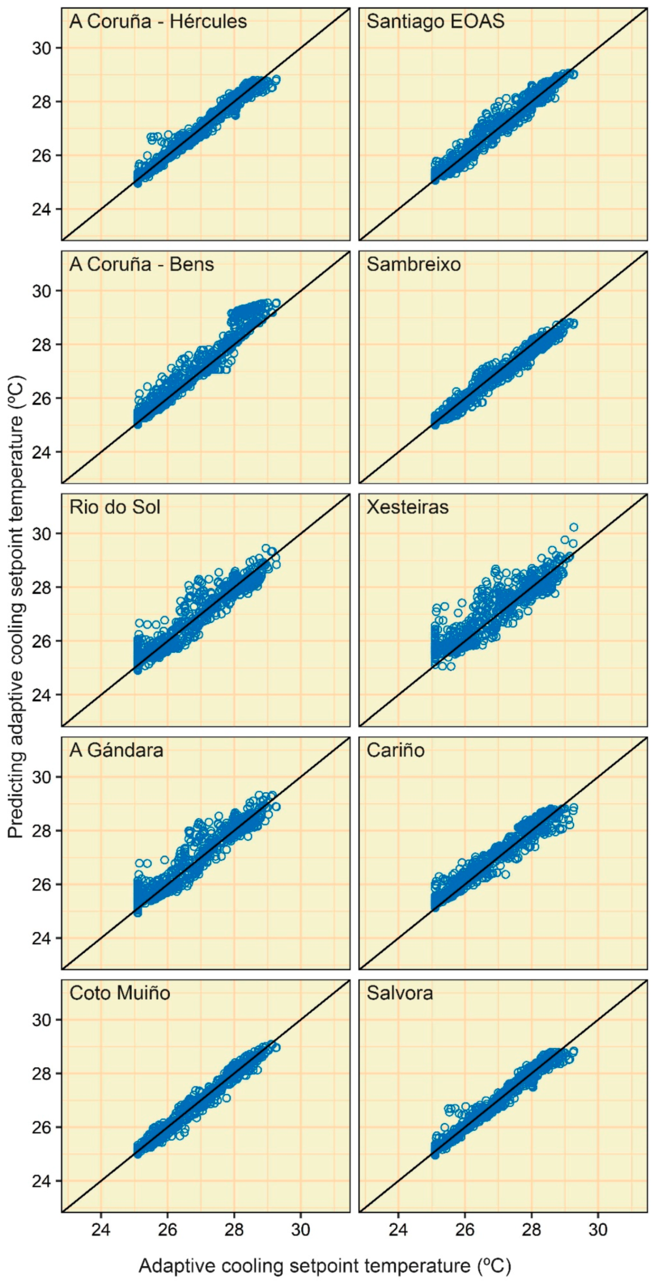
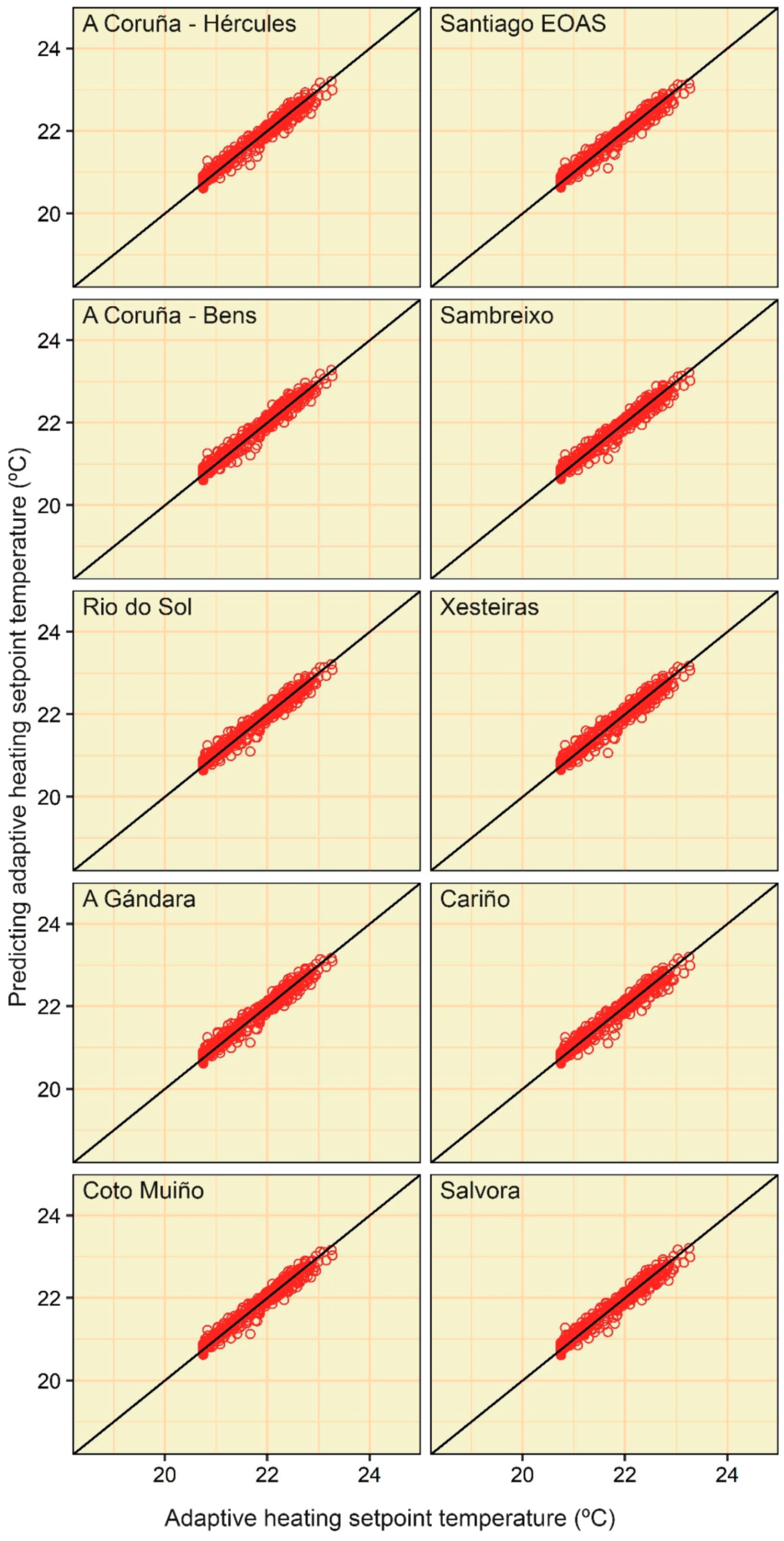
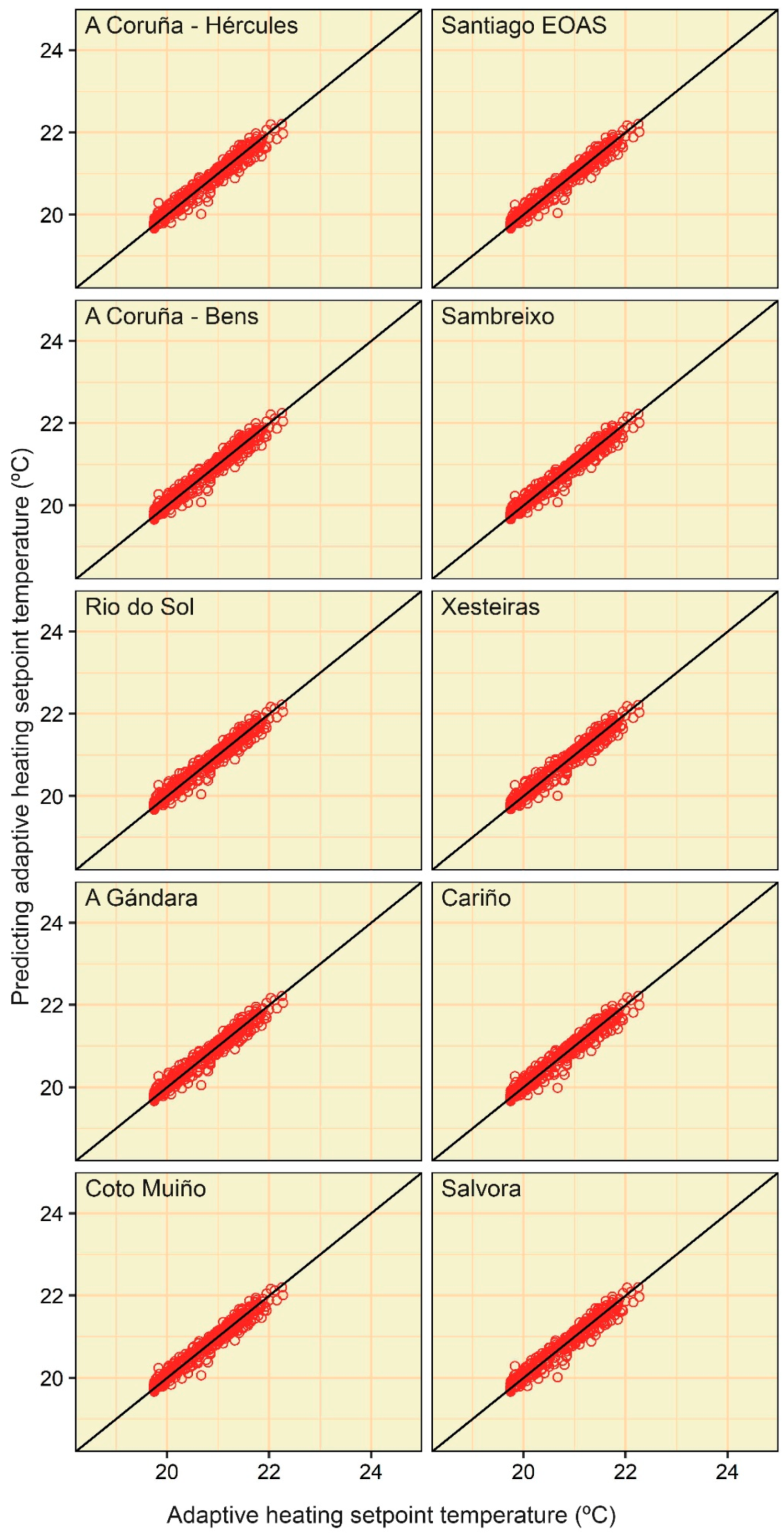
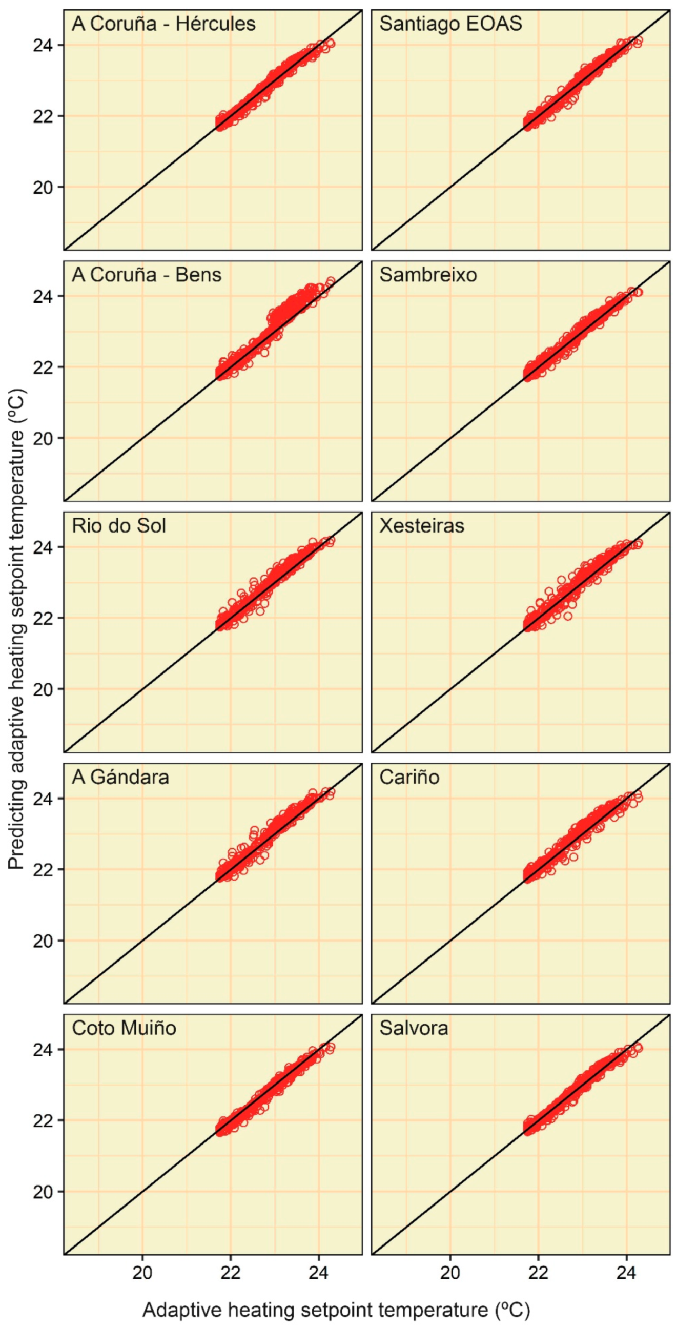
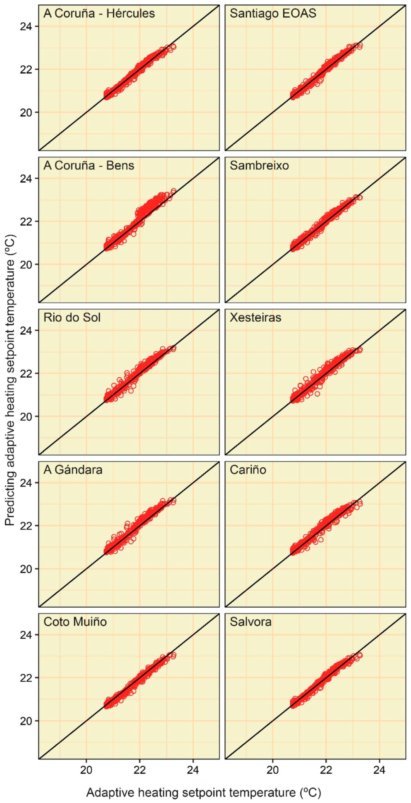
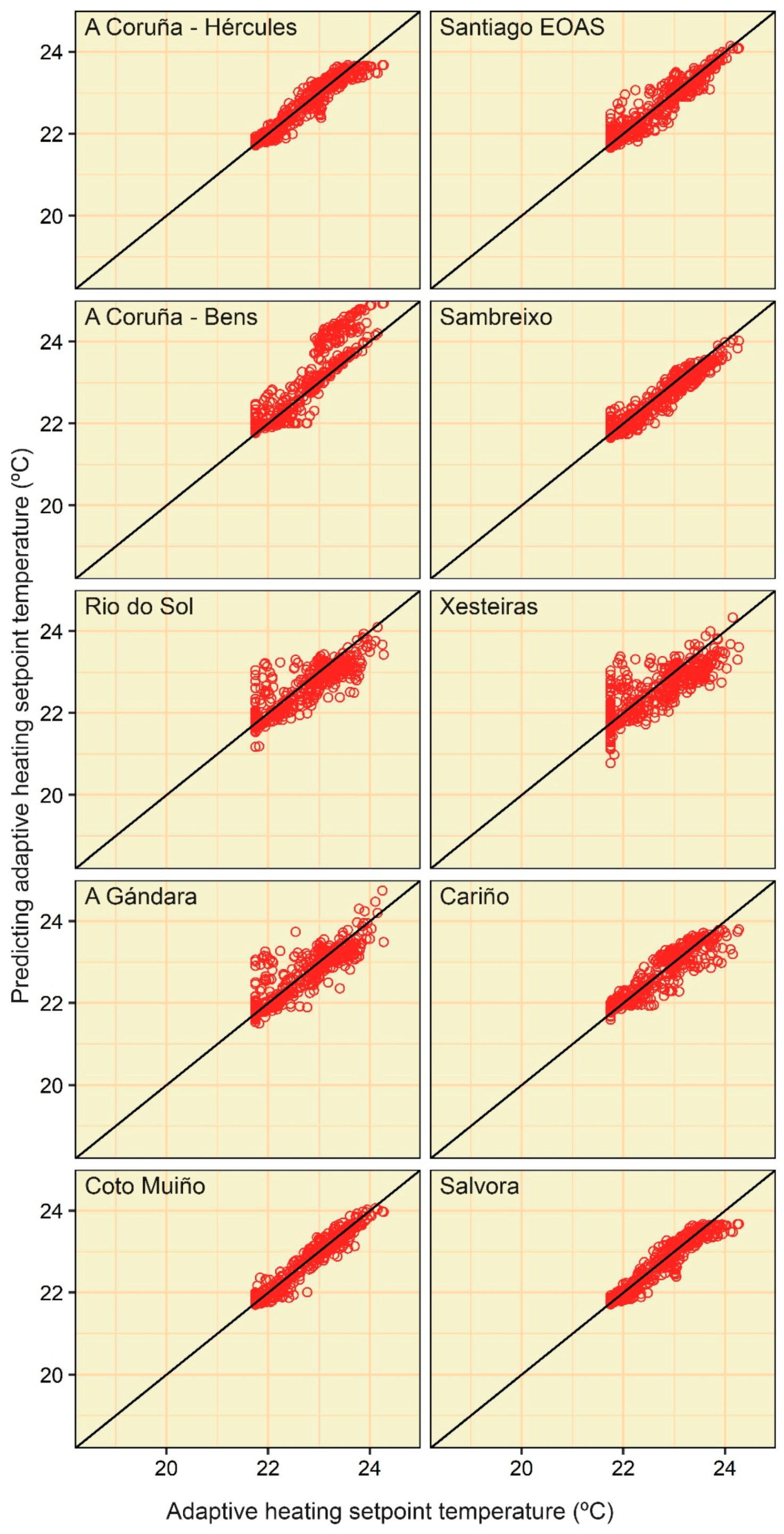
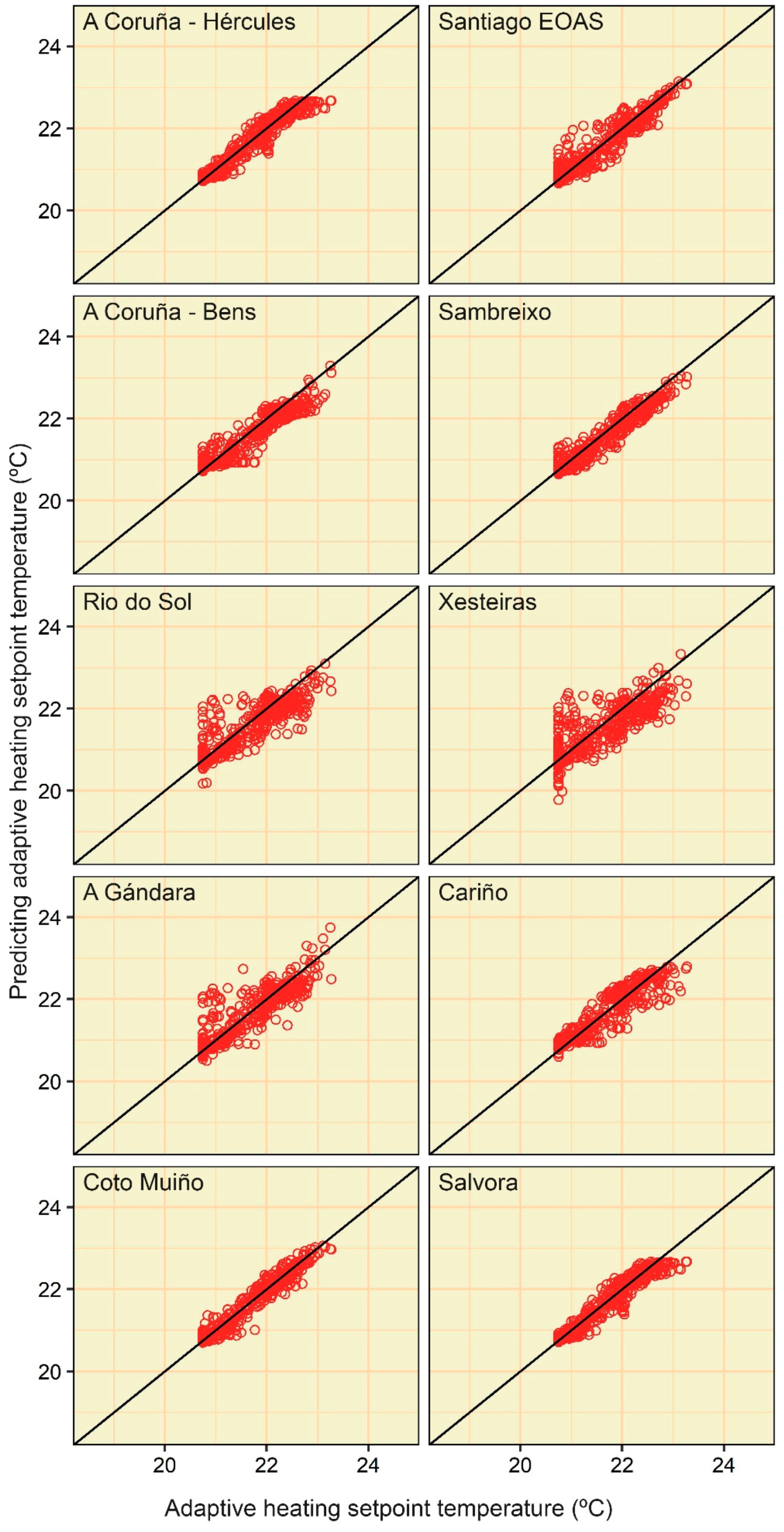
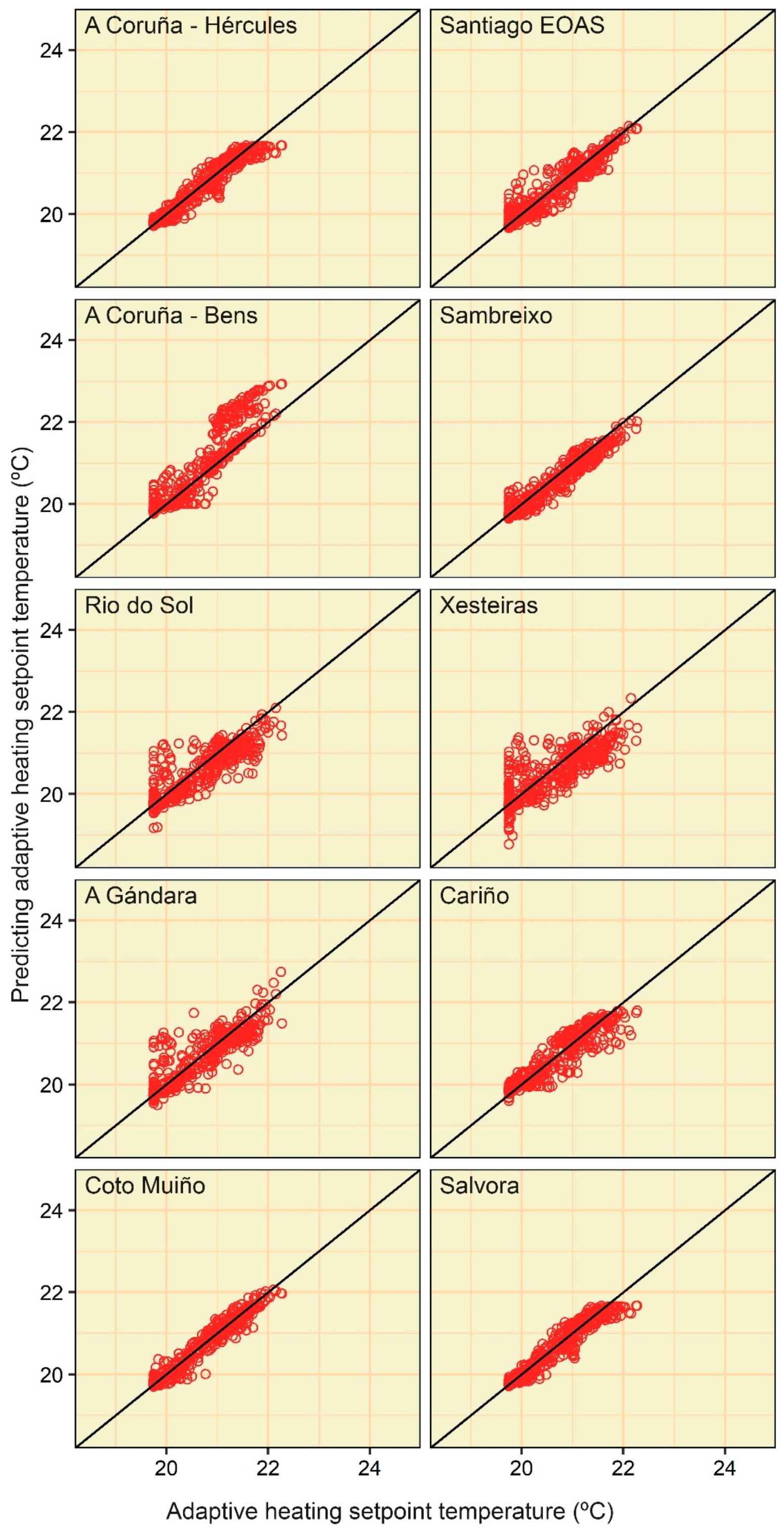
3. Results and Discussion
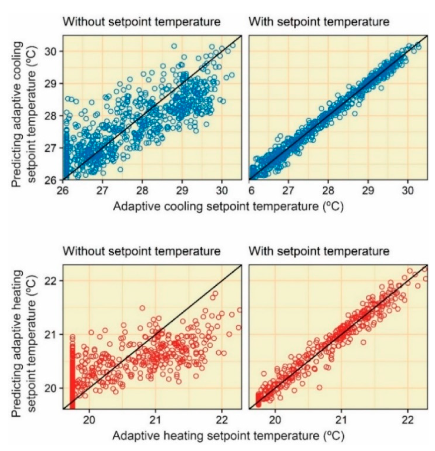
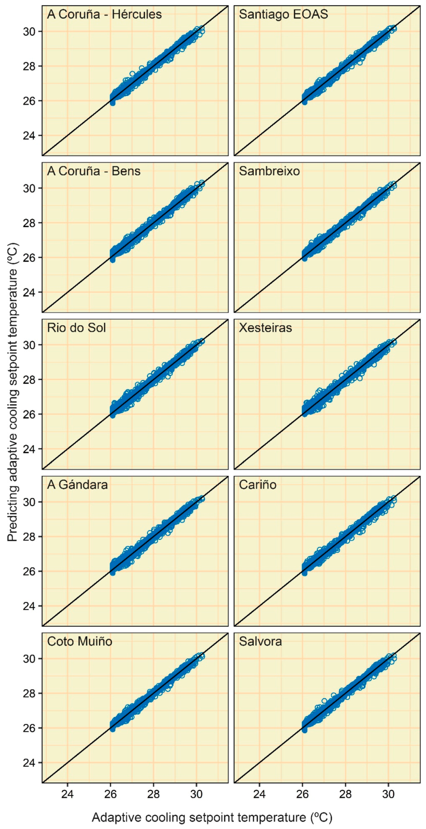
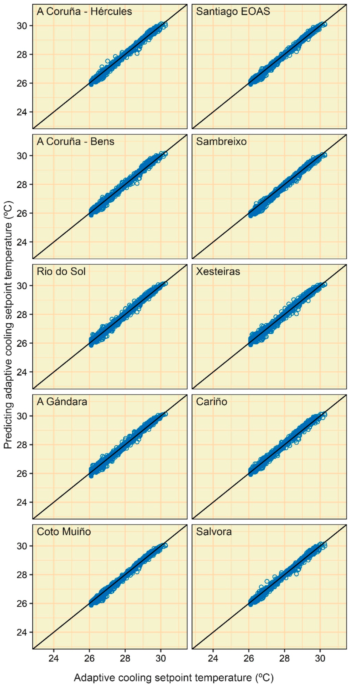
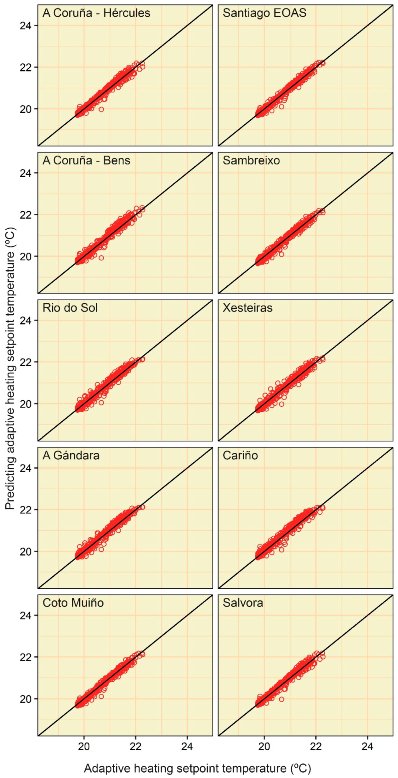
3.1. Approach 1: With the Setpoint Temperature and the External Temperature from the Previous Day
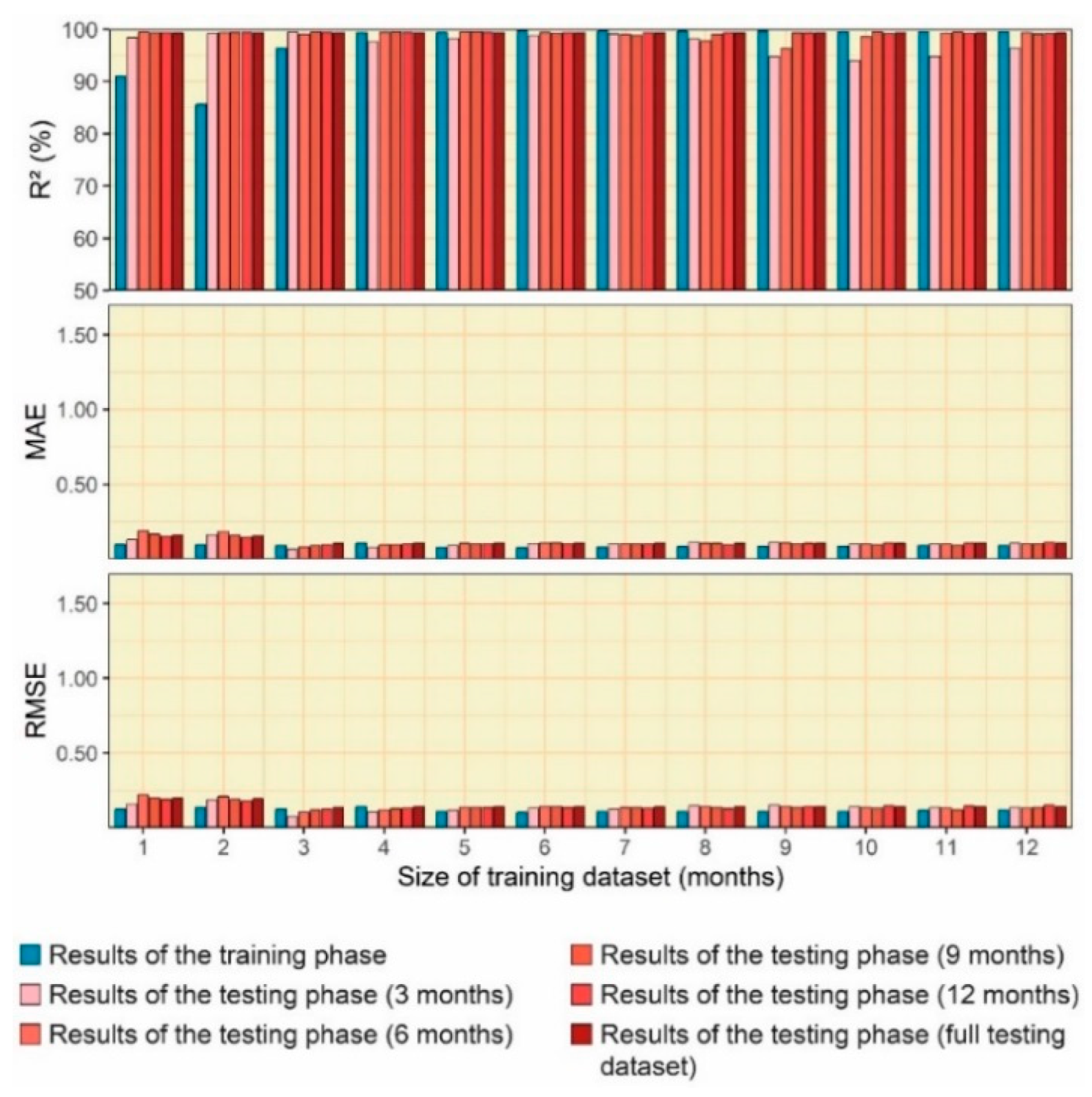
3.1.1. MLR
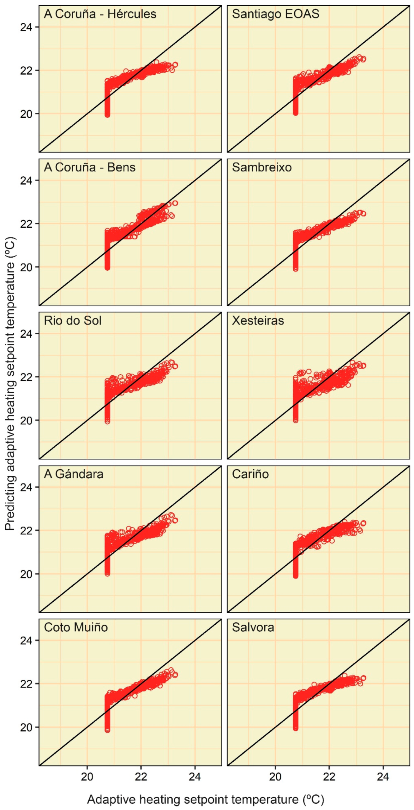
3.1.2. MLP
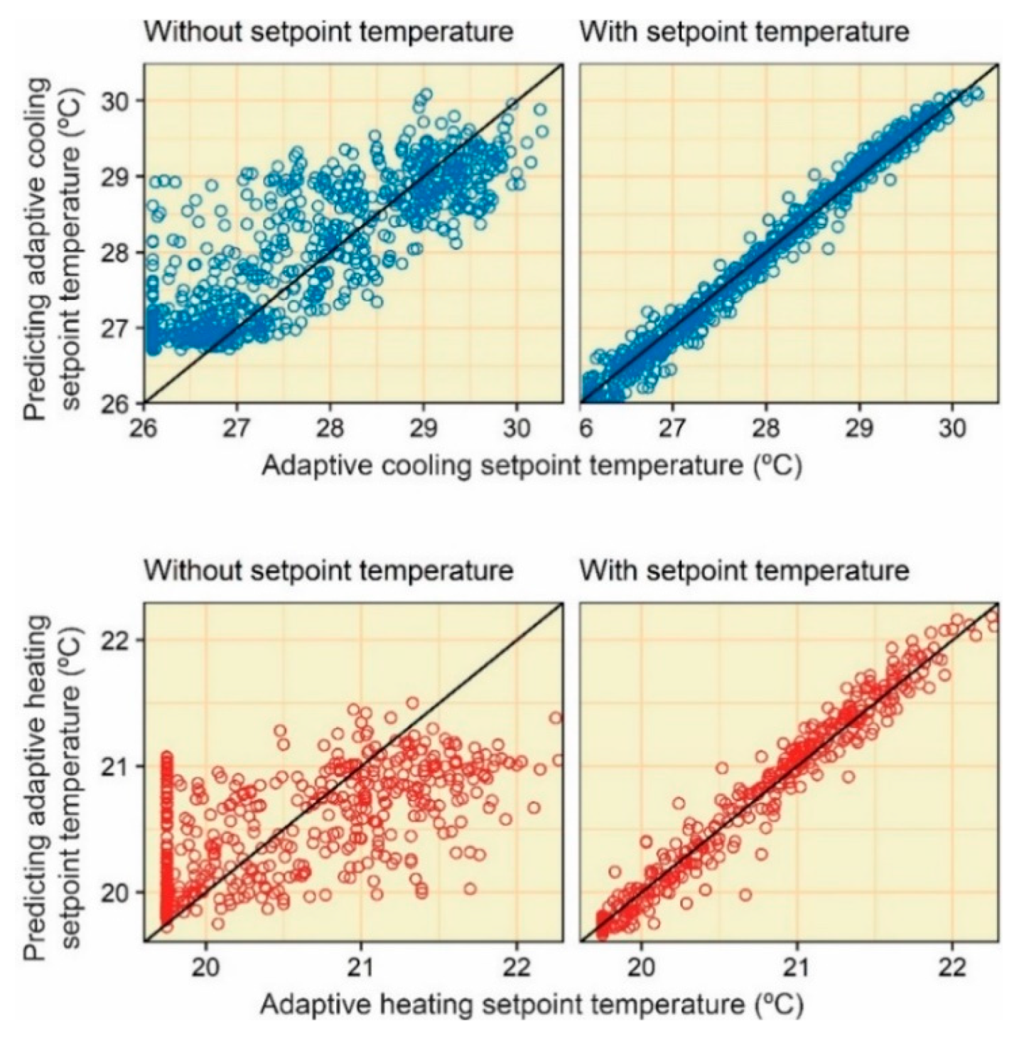
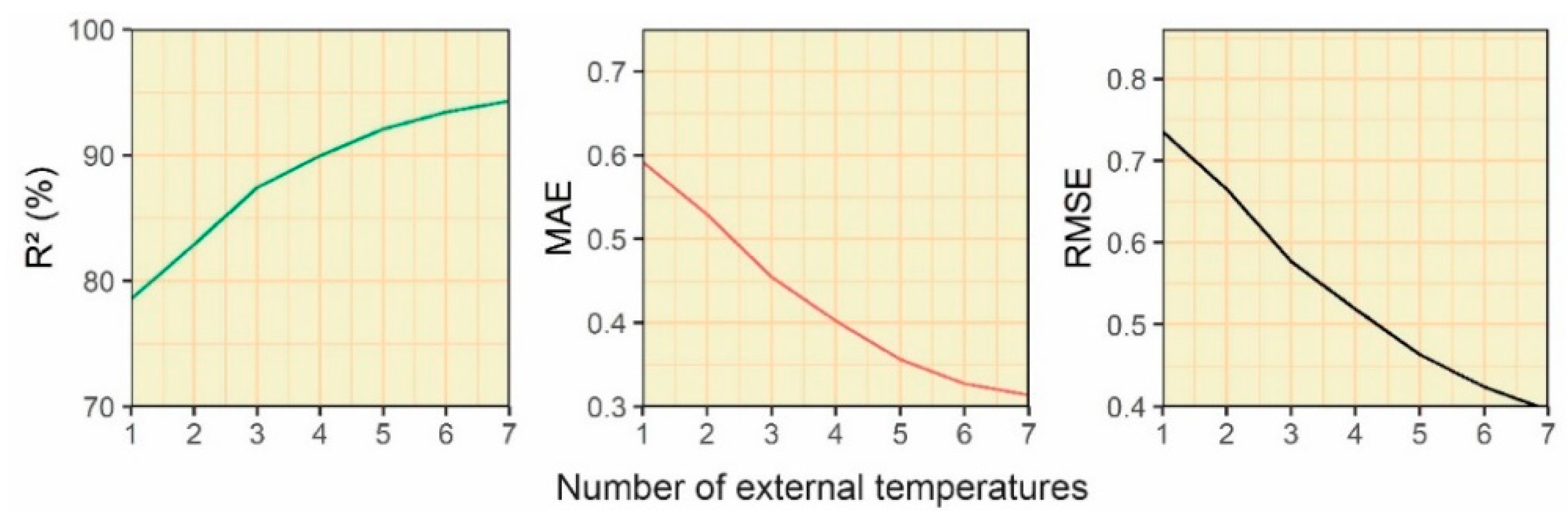
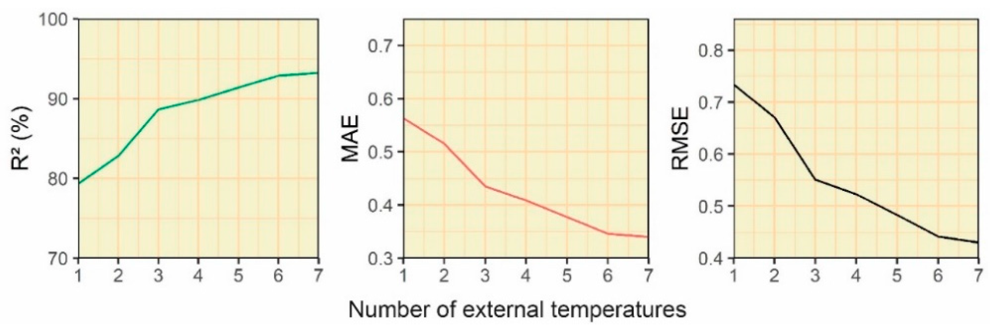
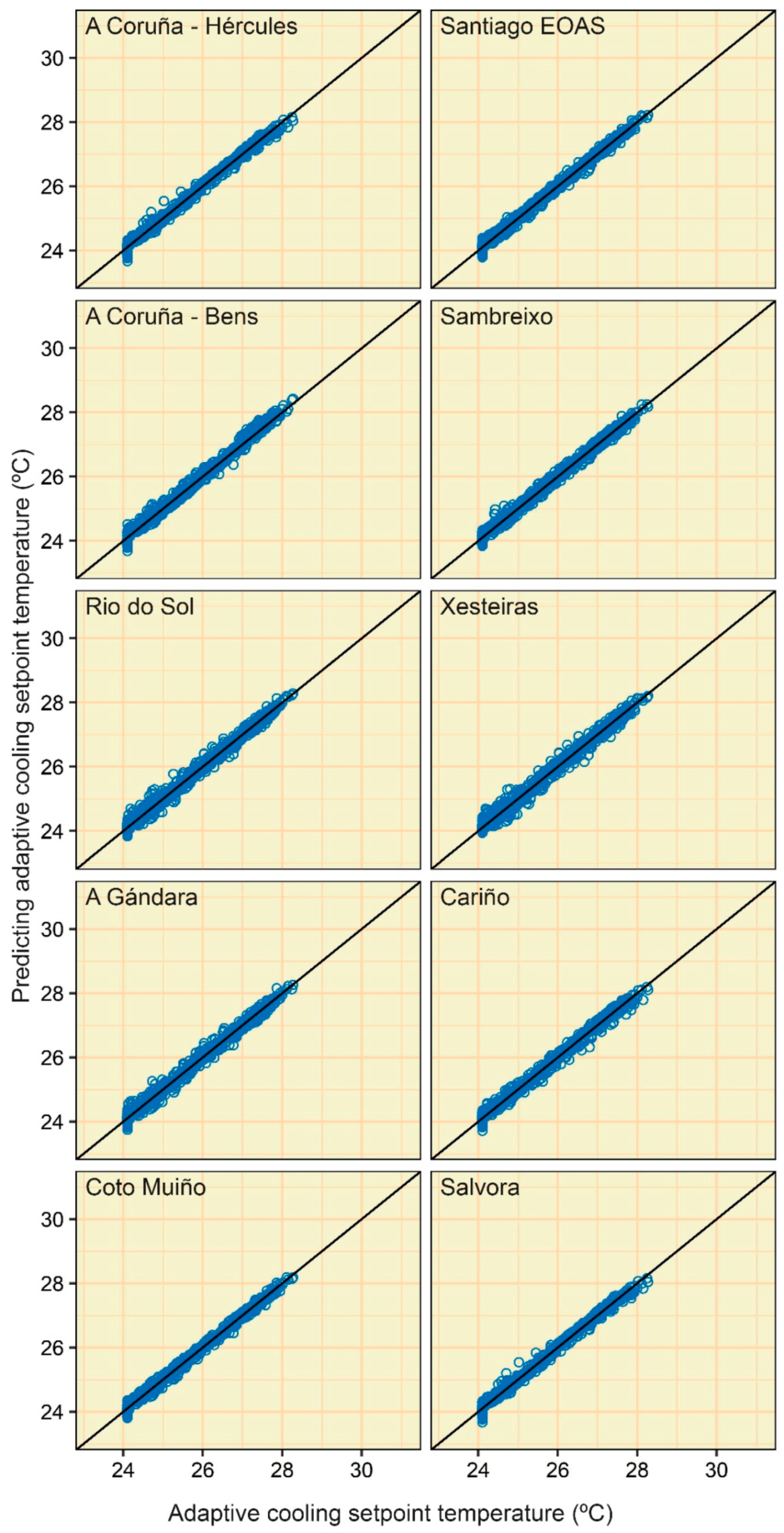
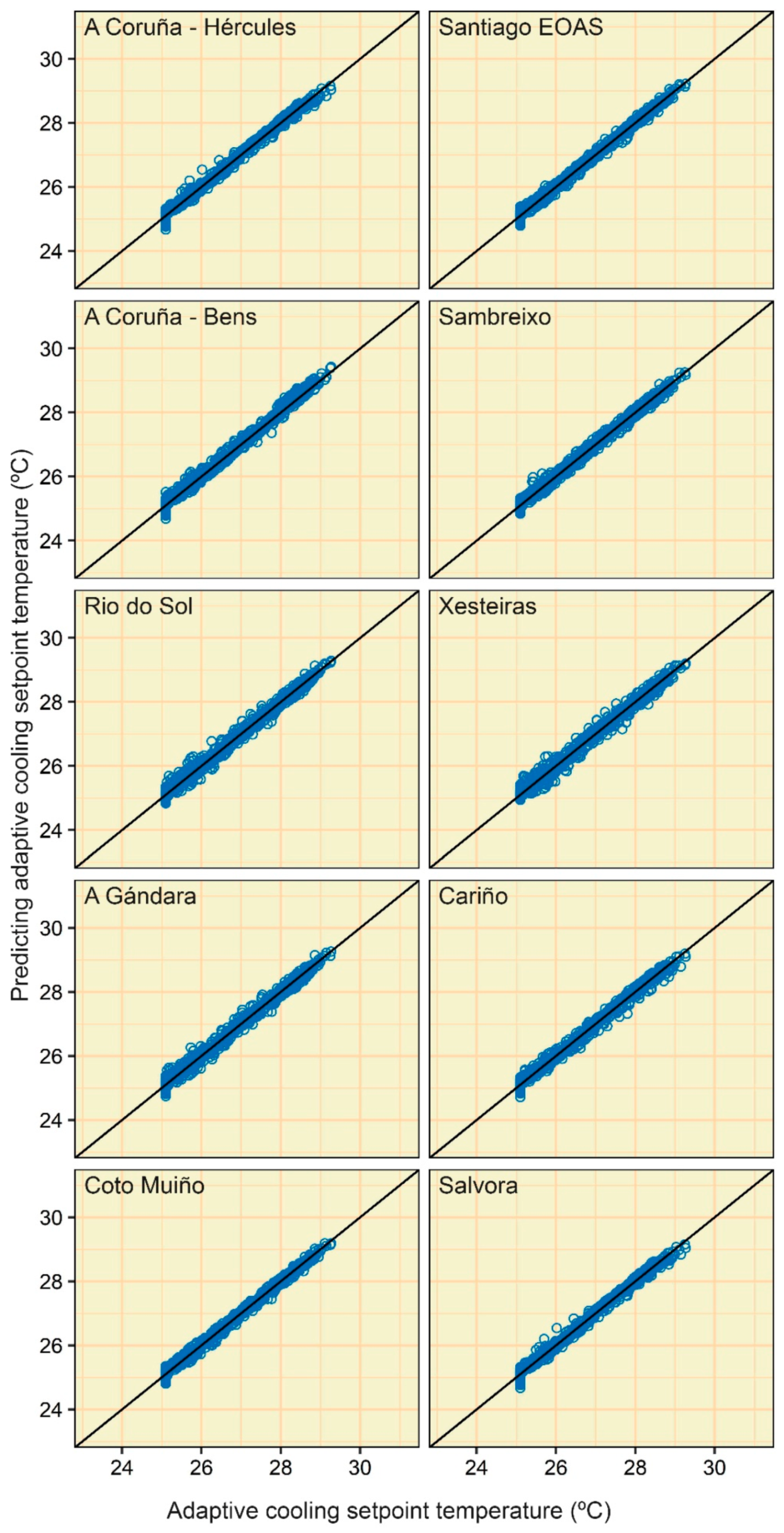
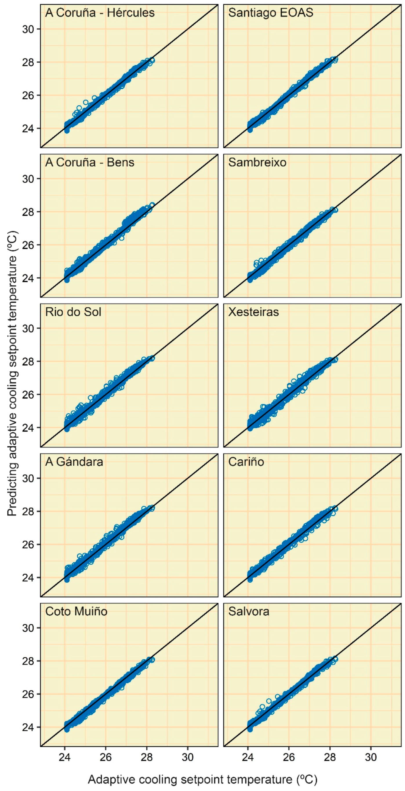
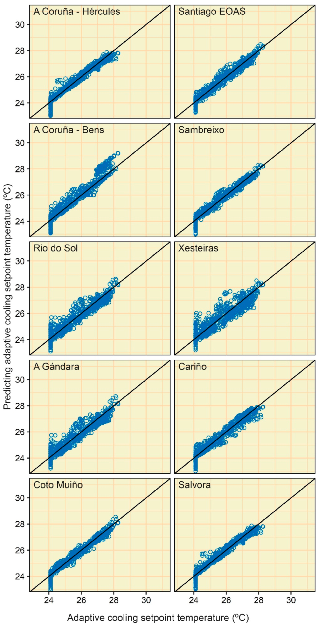
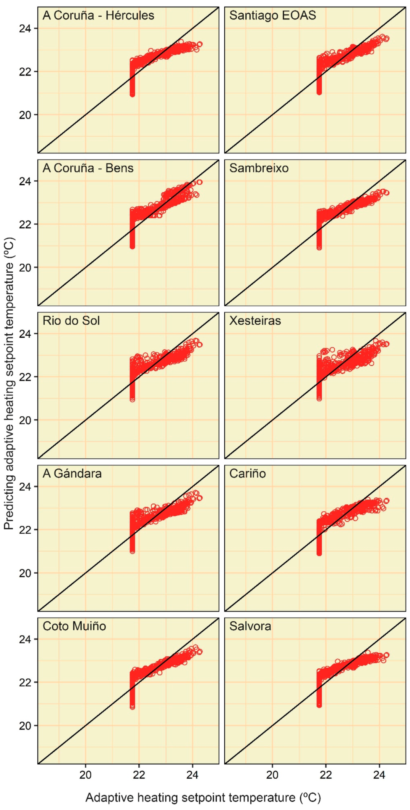
3.2. Approach 2: With Average Temperatures of the Last Seven Days
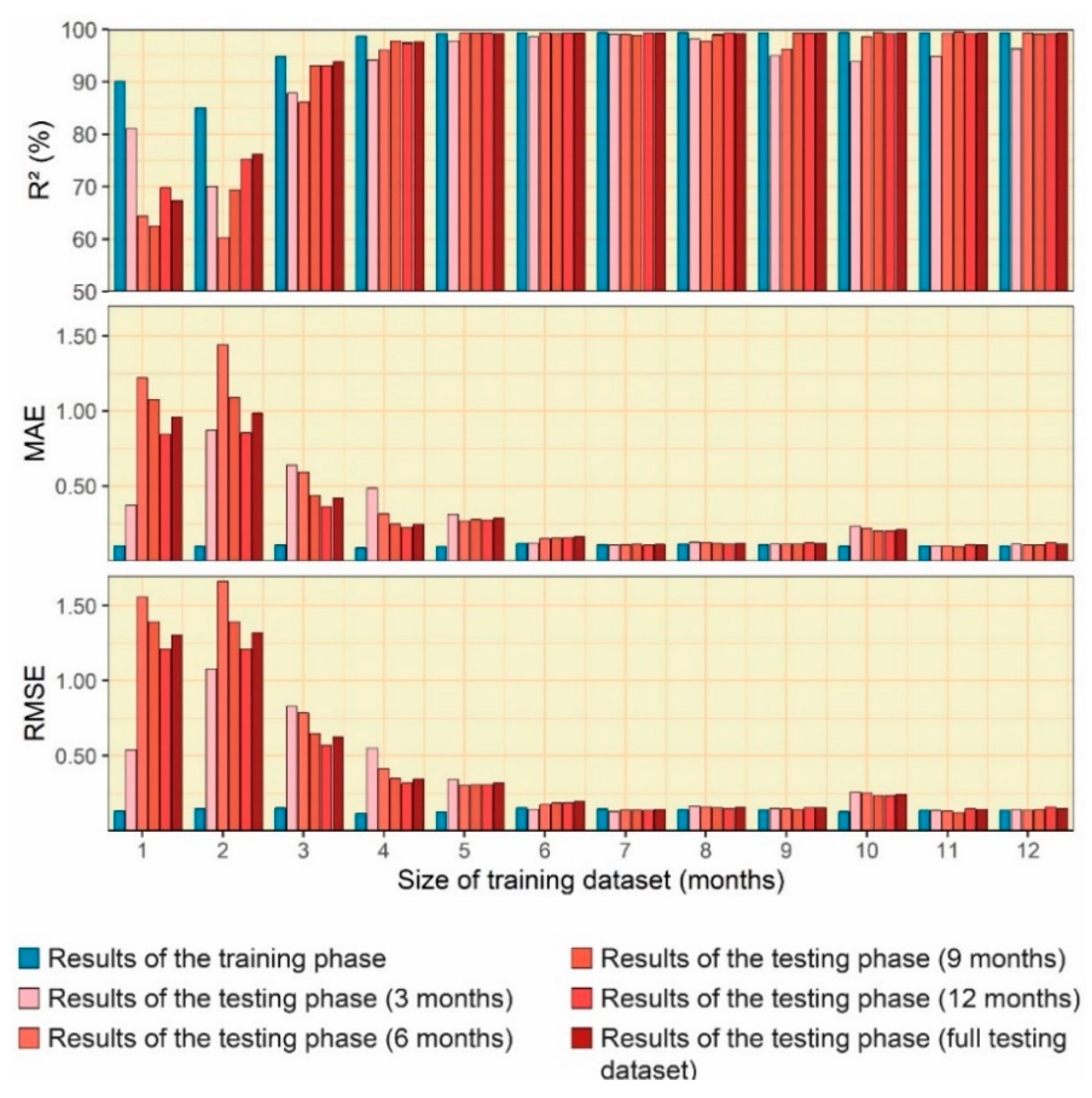
3.2.1. MLR
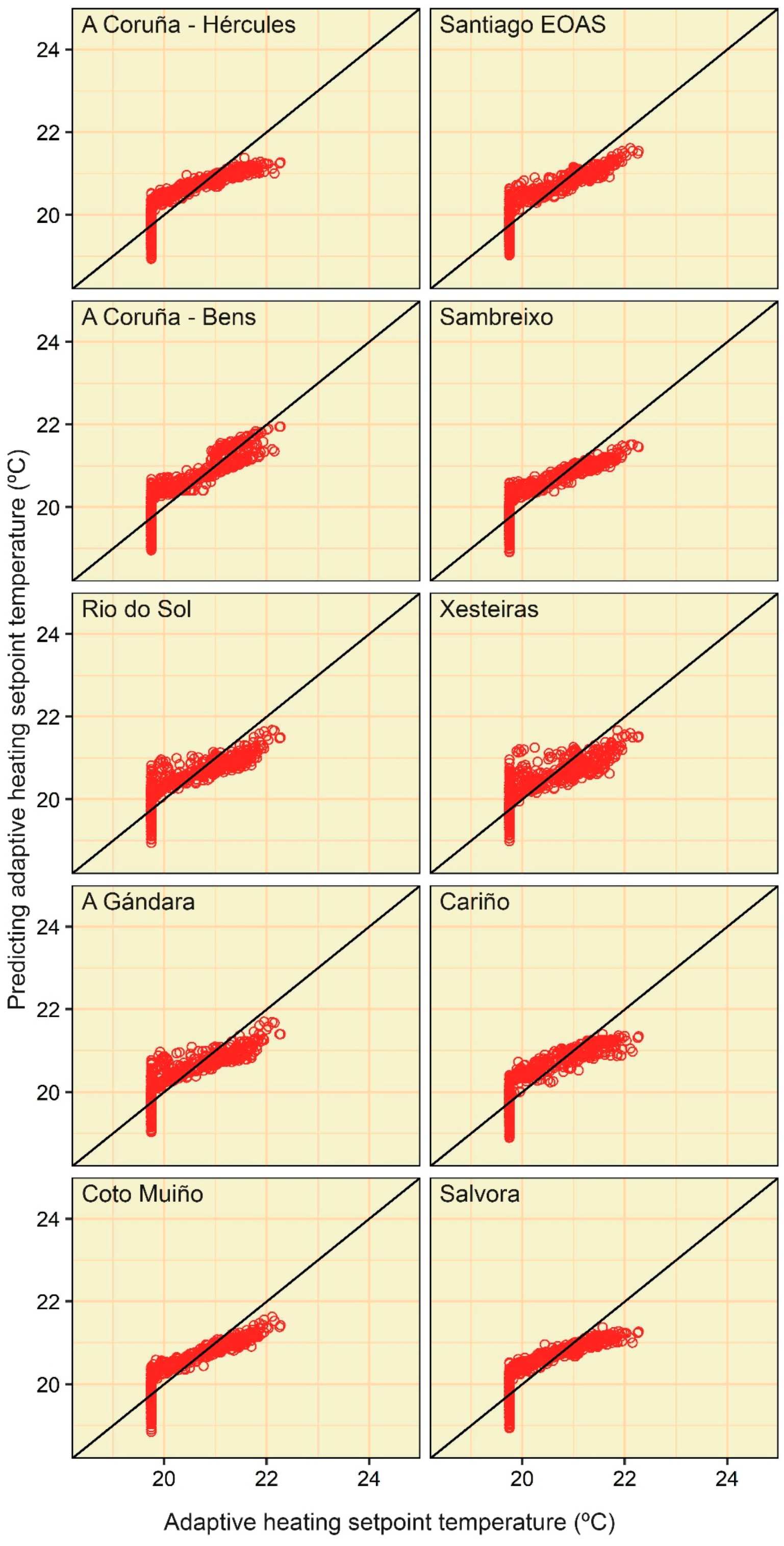
3.2.2. MLP
3.3. Estimation Methodology of the Adaptive Setpoint Temperatures
4. Conclusions
- The approach which used the values of setpoint temperature and mean daily external temperature from the previous day to estimate adaptive setpoint temperatures carried out estimations close to the actual values by using both data from all weather stations and two regression algorithms. In this way, the only difference between such algorithms was the time required to generate models with an adequate performance (1 month for the multivariable linear regression models and 5 months or more for multilayer perceptrons). This is useful to guarantee the feasibility of using MLRs to carry out estimations with an appropriate degree of accuracy.
- The approach which used the average values of the external temperature from the previous 7 days had different behaviour with respect to the other approach: only multilayer perceptrons obtained adequate performances, whereas the multivariable linear regression models obtained low correlation coefficients both in the training and testing phases. This was due to the limitations presented by the multivariable linear regression models when the adaptive setpoint temperatures were estimated not within the applicability of EN 15251 in the intervals of the running mean temperature. However, this aspect did not decrease the accuracy of the estimations carried out using the multilayer perceptrons, and accurate models could be obtained with training datasets of at least 6 months.
Author Contributions
Funding
Acknowledgments
Conflicts of Interest
Appendix A


References
- World Wildlife Fund. Living Planet Report 2014: Species and Spaces, People and Places; WWF International: Gland, Switzerland, 2014; Volume 1, ISBN 9780874216561. [Google Scholar]
- The United Nations Environment Programme. Building Design and Construction: Forging Resource Efficiency and Sustainable; The United Nations Environment Programme: Nairobi, Kenya, 2012. [Google Scholar]
- European Commission Directive 2002/91/EC of the European Parliament and of the council of 16 December 2002 on the energy performance of buildings. Off. J. Eur. Union 2002, 65–71. [CrossRef]
- European Union. Directive 2010/31/EU of the European Parliament and of the Council of 19 May 2010 on the Energy Performance of Buildings; European Union: Brussels, Belgium, 2010; Volume 153, pp. 13–35. [Google Scholar]
- Thomson, H.; Snell, C. Quantifying the prevalence of fuel poverty across the European Union. Energy Policy 2013, 52, 563–572. [Google Scholar] [CrossRef]
- Basu, R.; Samet, J.M. Relation between elevated ambient temperature and mortality: A review of the epidemiologic evidence. Epidemiol. Rev. 2002, 24, 190–202. [Google Scholar] [CrossRef]
- Basu, R. High ambient temperature and mortality: A review of epidemiologic studies from 2001 to 2008. Environ. Health 2009, 8, 40. [Google Scholar] [CrossRef]
- European Commission. A Roadmap for Moving to a Competitive Low Carbon Economy in 2050; European Commission: Brussels, Belgium, 2011; pp. 1–15. [Google Scholar]
- International Energy Agency. Energy Efficiency 2017; International Energy Agency: Paris, France, 2017. [Google Scholar] [CrossRef]
- Spanish Institute of Statistics Population and Housing Census. Available online: https://www.ine.es/censos2011_datos/cen11_datos_resultados.htm# (accessed on 9 November 2018).
- The Government of Spain. Royal Decree 314/2006. Approving the Spanish Technical Building Code CTE-DB-HE-1; The Government of Spain: Madrid, Spain, 2013.
- Rafsanjani, H.N.; Ahn, C.R.; Alahmad, M. A review of approaches for sensing, understanding, and improving occupancy-related energy-use behaviors in commercial buildings. Energies 2015, 8, 10996–11029. [Google Scholar] [CrossRef]
- Sánchez-García, D.; Rubio-Bellido, C.; Martín del Río, J.; Pérez-Fargallo, A. Towards the quantification of energy demand and consumption through the adaptive comfort approach in mixed mode office buildings considering climate change. Energy Build. 2019. [Google Scholar] [CrossRef]
- Sánchez-García, D.; Rubio-Bellido, C.; Marrero Meléndez, M.; Guevara-García, F.J.; Canivell, J. El control adaptativo en instalaciones existentes y su potencial en el contexto del cambio climático. Habitat Sustentable 2017, 7, 6–17. [Google Scholar] [CrossRef]
- Sánchez-Guevara Sánchez, C.; Mavrogianni, A.; Neila González, F.J. On the minimal thermal habitability conditions in low income dwellings in Spain for a new definition of fuel poverty. Build. Environ. 2017, 114, 344–356. [Google Scholar] [CrossRef]
- Spyropoulos, G.N.; Balaras, C.A. Energy consumption and the potential of energy savings in Hellenic office buildings used as bank branches—A case study. Energy Build. 2011, 43, 770–778. [Google Scholar] [CrossRef]
- Yun, G.Y.; Lee, J.H.; Steemers, K. Extending the applicability of the adaptive comfort model to the control of air-conditioning systems. Build. Environ. 2016, 105, 13–23. [Google Scholar] [CrossRef]
- Hoyt, T.; Arens, E.; Zhang, H. Extending air temperature setpoints: Simulated energy savings and design considerations for new and retrofit buildings. Build. Environ. 2014, 88, 89–96. [Google Scholar] [CrossRef]
- Humphreys, M.A.; Rijal, H.B.; Nicol, J.F. Updating the adaptive relation between climate and comfort indoors; new insights and an extended database. Build. Environ. 2013, 63, 40–55. [Google Scholar] [CrossRef]
- de Dear, R.; Brager, G.S. Thermal comfort in naturally ventilated buildings: Revision to ASHRAE standards 55. J. Energy Build. 2002, 34, 549–561. [Google Scholar] [CrossRef]
- CEN. EN 15251:2007 Indoor Environmental Input Parameters for Design and Assessment of Energy Performance of Buildings Addressing Indoor Quality, Thermal Environment, Lighting and Acoustics; European Committee for Standardization: Brussels, Belgium, 2007. [Google Scholar]
- Attia, S.; Carlucci, S. Impact of different thermal comfort models on zero energy residential buildings in hot climate. Energy Build. 2015, 102, 117–128. [Google Scholar] [CrossRef]
- Hubbard, K.G.; Lin, X. Realtime data filtering models for air temperature measurements. Geophys. Res. Lett. 2002, 29. [Google Scholar] [CrossRef]
- Albrecht, F. Thermometer zur Messung der wahren Lufttemperatur. Meteorol. Z. 1927, 24, 420–424. [Google Scholar]
- Albrecht, F. Über die Einwirkung der Strahling auf frei aufgestellte elektrische Thermometer. Veröff. Pruss. Meteorol. Inst. 1934, 402, 76–82. [Google Scholar]
- Fuchs, M.; Tanner, C.B. Radiation shields for air temperature thermometers. J. Appl. Meteorol. 1965, 4, 544–547. [Google Scholar] [CrossRef]
- Anderson, S.P.; Baumgartner, M.F. Radiative heating errors in naturally ventilated air temperature measurements made from buoys. J. Atmos. Ocean. Technol. 1998, 15, 157–173. [Google Scholar] [CrossRef]
- Huwald, H.; Higgins, C.W.; Boldi, M.O.; Bou-Zeid, E.; Lehning, M.; Parlange, M.B. Albedo effect on radiative errors in air temperature measurements. Water Resour. Res. 2009, 45, 1–13. [Google Scholar] [CrossRef]
- Arck, M.; Scherer, D. A physically based method for correcting temperature data measured by naturally ventilated sensors over snow. J. Glaciol. 2001, 47, 665–670. [Google Scholar] [CrossRef]
- Georges, C.; Kaser, G. Ventilated and unventilated air temperature measurements for glacier-climate studies on a tropical high mountain site. J. Geophys. Res. Atmos. 2002, 107, 1–11. [Google Scholar] [CrossRef]
- Nakamura, R.; Mahrt, L. Air temperature measurement errors in naturally ventilated radiation shields. J. Atmos. Ocean. Technol. 2005, 22, 1046–1058. [Google Scholar] [CrossRef]
- Hardy, D.R.; Vuille, M.; Braun, G.; Keimig, F.; Bradley, R.S. Annual and Daily Meteorological Cycles at High Altitude on a Tropical Mountain. Bull. Am. Meteorol. Soc. 1998, 79, 1899–1913. [Google Scholar] [CrossRef]
- Lundquist, J.D.; Huggett, B. Evergreen trees as inexpensive radiation shields for temperature sensors. Water Resour. Res. 2010, 46, 1–5. [Google Scholar] [CrossRef]
- World Meteorological Organization. Guide to Meteorological Instruments and Methods of Observation; World Meteorological Organization: Geneva, Switzerland, 2008; ISBN 9789263100085. [Google Scholar]
- Erell, E.; Leal, V.; Maldonado, E. Measurement of air temperature in the presence of a large radiant flux: An assessment of passively ventilated thermometer screens. Bound.-Layer Meteorol. 2005, 114, 205–231. [Google Scholar] [CrossRef]
- Spanish Institute of Statistics Surface Extension of the Autonomous Communities and Provinces, by Altimetric Zones. Available online: http://www.ine.es/inebaseweb/pdfDispacher.do?td=154090&L=0 (accessed on 10 January 2019).
- Spanish Institute of Statistics Population by Autonomous Communities and Cities And Sex. Available online: https://www.ine.es/jaxiT3/Tabla.htm?t=2853&L=0 (accessed on 10 January 2019).
- Rubel, F.; Kottek, M. Observed and projected climate shifts 1901-2100 depicted by world maps of the Köppen-Geiger climate classification. Meteorol. Z. 2010, 19, 135–141. [Google Scholar] [CrossRef]
- Dahlgren, R.A.; Boettinger, J.L.; Huntington, G.L.; Amundson, R.G. Soil development along an elevational transect in the western Sierra Nevada, California. Geoderma 1997, 78, 207–236. [Google Scholar] [CrossRef]
- Franzmeier, D.P.; Pedersen, E.J.; Longwell, T.J.; Byrne, J.G.; Losche, C.K. Properties of Some Soils in the Cumberland Plateau as Related to Slope Aspect and Position1. Soil Sci. Soc. Am. J. 1969, 33, 755–761. [Google Scholar] [CrossRef]
- Tsui, C.C.; Chen, Z.S.; Hsieh, C.F. Relationships between soil properties and slope position in a lowland rain forest of southern Taiwan. Geoderma 2004, 123, 131–142. [Google Scholar] [CrossRef]
- Yimer, F.; Ledin, S.; Abdelkadir, A. Soil property variations in relation to topographic aspect and vegetation community in the south-eastern highlands of Ethiopia. For. Ecol. Manag. 2006, 232, 90–99. [Google Scholar] [CrossRef]
- Eguía Oller, P.; Alonso Rodríguez, J.M.; Saavedra González, Á.; Arce Fariña, E.; Granada Álvarez, E. Improving the calibration of building simulation with interpolated weather datasets. Renew. Energy 2018, 122, 608–618. [Google Scholar] [CrossRef]
- Ahmad, A.; Maslehuddin, M.; Al-Hadhrami, L.M. In situ measurement of thermal transmittance and thermal resistance of hollow reinforced precast concrete walls. Energy Build. 2014, 84, 132–141. [Google Scholar] [CrossRef]
- Pino-Mejías, R.; Pérez-Fargallo, A.; Rubio-Bellido, C.; Pulido-Arcas, J.A. Comparison of linear regression and artificial neural networks models to predict heating and cooling energy demand, energy consumption and CO2 emissions. Energy 2017, 118, 24–36. [Google Scholar] [CrossRef]
- Pulido-Arcas, J.A.; Pérez-Fargallo, A.; Rubio-Bellido, C. Multivariable regression analysis to assess energy consumption and CO2 emissions in the early stages of offices design in Chile. Energy Build. 2016, 133, 738–753. [Google Scholar] [CrossRef]
- Qiang, G.; Zhe, T.; Yan, D.; Neng, Z. An improved office building cooling load prediction model based on multivariable linear regression. Energy Build. 2015, 107, 445–455. [Google Scholar] [CrossRef]
- Amber, K.P.; Aslam, M.W.; Mahmood, A.; Kousar, A.; Younis, M.Y.; Akbar, B.; Chaudhary, G.Q.; Hussain, S.K. Energy consumption forecasting for university sector buildings. Energies 2017, 10, 1579. [Google Scholar] [CrossRef]
- Kialashaki, A.; Reisel, J.R. Modeling of the energy demand of the residential sector in the United States using regression models and artificial neural networks. Appl. Energy 2013, 108, 271–280. [Google Scholar] [CrossRef]
- Asadi, S.; Amiri, S.S.; Mottahedi, M. On the development of multi-linear regression analysis to assess energy consumption in the early stages of building design. Energy Build. 2014, 85, 246–255. [Google Scholar] [CrossRef]
- Wasserman, P.D. Neural computing: Theory and practice. N. Y. Van Nostrand Reinhold 1989. [Google Scholar] [CrossRef]
- Kandananond, K. Forecasting electricity demand in Thailand with an artificial neural network approach. Energies 2011, 4, 1246–1257. [Google Scholar] [CrossRef]
- Pino-Mejías, R.; Pérez-Fargallo, A.; Rubio-Bellido, C.; Pulido-Arcas, J.A. Artificial neural networks and linear regression prediction models for social housing allocation: Fuel Poverty Potential Risk Index. Energy 2018, 164, 627–641. [Google Scholar] [CrossRef]
- Attoue, N.; Shahrour, I.; Younes, R. Smart building: Use of the artificial neural network approach for indoor temperature forecasting. Energies 2018, 11, 395. [Google Scholar] [CrossRef]
- Zabada, S.; Shahrour, I. Analysis of heating expenses in a large social housing stock using artificial neural networks. Energies 2017, 10, 2086. [Google Scholar] [CrossRef]
- Yu, W.; Li, B.; Lei, Y.; Liu, M. Analysis of a residential building energy consumption demand model. Energies 2011, 4, 475–487. [Google Scholar] [CrossRef]
- Deb, C.; Eang, L.S.; Yang, J.; Santamouris, M. Forecasting diurnal cooling energy load for institutional buildings using Artificial Neural Networks. Energy Build. 2016, 121, 284–297. [Google Scholar] [CrossRef]
- Moon, J.W.; Chin, K.-I.; Kim, S. Optimum application of thermal factors to artificial neural network models for improvement of control performance in double skin-enveloped buildings. Energies 2013, 6, 4223–4245. [Google Scholar] [CrossRef]
- Akaike, H. A New Look at the Statistical Model Identification. IEEE Trans. Autom. Control 1974. [Google Scholar] [CrossRef]
- Bienvenido-Huertas, D.; Moyano, J.; Rodríguez-Jiménez, C.E.; Marín, D. Applying an artificial neural network to assess thermal transmittance in walls by means of the thermometric method. Appl. Energy 2019, 233–234, 1–14. [Google Scholar] [CrossRef]
- Fletcher, R. Practical Methods of Optimization; John Wiley & Sons: Chichester, UK; New York, NY, USA; Brisbane, Australia; Toronto, ON, Canada, 1980; ISBN 9780471277118. [Google Scholar]
- Kohavi, R. A Study of Cross-Validation and Bootstrap for Accuracy Estimation and Model Selection. In Proceedings of the International Joint Conference on Artificial Intelligence, Montreal, QC, Canada, 20–25 August 1995; Volume 5. [Google Scholar]


| Categories | Description | |
|---|---|---|
| I | High level of expectation. The standard recommends its use in buildings occupied by weak and sensitive people, with special requirements (e.g., sick people, children or elderly). | 2 |
| II | Normal level of expectation. The standard recommends its use in new and renovated buildings. | 3 |
| III | Moderate level of expectation. The standard recommends its use in existing buildings. | 4 |
| Technical Specification | Values |
|---|---|
| Measurement Range | −50 to 100 °C (default −40 to 60 °C) |
| Output Signal Range | 0 to 1 V |
| Accuracy | ±0.1 °C with standard configuration settings (at 23 °C) |
| Long-Term Stability | <0.1 °C/year |
| Weather Station | Latitude a | Longitude a | Altitude (m) | Distance from the Case Study (m) | Height Difference with Respect to the Case Study (m) |
|---|---|---|---|---|---|
| 1. Coruña-Hercules | 43.3829 | −8.40993 | 21 | 5883.02 | −34 |
| 2. Coruña-Bens | 43.3634 | −8.44187 | 131 | 4438.60 | 76 |
| 3. Rio do Sol | 43.0952 | −8.69099 | 540 | 34,549.61 | 485 |
| 4. A Gándara | 43.1081 | −9.05694 | 405 | 57,808.57 | 350 |
| 5. Coto Muiño | 43.028873 | −8.974914 | 317 | 56,622.68 | 262 |
| 6. Santiago EOAS | 42,876 | −8.55944 | 255 | 51,887.22 | 200 |
| 7. Sambreixo | 43.1457 | −7.79112 | 496 | 54,295.09 | 441 |
| 8. Xesteiras | 42.6756 | −8.58618 | 715 | 74,136.00 | 660 |
| 9. Cariño | 43,734 | −7.86335 | 5 | 63,029.12 | −50 |
| 10. Salvora | 42.4649 | −9.01364 | 24 | 107,967.54 | −31 |
| Sensor | Measurement Range | Accuracy | Weather Station |
|---|---|---|---|
| Vaisala HMP155 | −80–60 °C | ±0.25 °C | Coruña-Hércules, Coruña-Bens, Rio do Sol, A Gándara, Coto Muiño, Sambreixo, Cariño, Salvora |
| Geónica STH-5031 | −40–60 °C | ±0.10 °C | Santiago EOAS |
| Rotronic HC2A-S3 | −50–100 °C | ±0.30 °C | Xesteiras |
| Approach | Input Variables | Output Variables |
|---|---|---|
| Approach 1 | a | a |
| Approach 2 | a |
| Dataset | Number of Instances (days) | First Date | Last Date |
|---|---|---|---|
| Training | 365 | 12 February 2016 | 11 February 2017 |
| Testing | 675 | 12 February 2017 | 17 December 2018 |
| Model | Upper Limit | Lower Limit | ||||
|---|---|---|---|---|---|---|
| Training | ||||||
| Coruña-Hercules | 99.71 | 0.0696 | 0.0911 | 99.01 | 0.0654 | 0.0936 |
| Coruña-Bens | 99.70 | 0.0694 | 0.0923 | 99.10 | 0.0650 | 0.0895 |
| Rio do Sol | 99.51 | 0.0887 | 0.1183 | 99.04 | 0.0640 | 0.0921 |
| A Gándara | 99.54 | 0.0876 | 0.1147 | 99.06 | 0.0642 | 0.0915 |
| Coto Muiño | 99.72 | 0.0689 | 0.0903 | 99.07 | 0.0649 | 0.0908 |
| Santiago EOAS | 99.72 | 0.0675 | 0.0901 | 99.07 | 0.0641 | 0.0911 |
| Sambreixo | 99.66 | 0.0774 | 0.0984 | 99.05 | 0.0651 | 0.0919 |
| Xesteiras | 99.36 | 0.1006 | 0.1356 | 99.00 | 0.0642 | 0.0940 |
| Cariño | 99.58 | 0.0815 | 0.1099 | 98.96 | 0.0643 | 0.0959 |
| Salvora | 99.71 | 0.0696 | 0.0911 | 99.01 | 0.0654 | 0.0936 |
| Testing | ||||||
| Coruña-Hercules | 99.61 | 0.0774 | 0.1087 | 99.18 | 0.0679 | 0.0956 |
| Coruña-Bens | 99.52 | 0.1249 | 0.1525 | 99.22 | 0.0695 | 0.0954 |
| Rio do Sol | 99.53 | 0.0906 | 0.1218 | 99.21 | 0.0674 | 0.0937 |
| A Gándara | 99.54 | 0.0927 | 0.1209 | 99.21 | 0.0671 | 0.0941 |
| Coto Muiño | 99.76 | 0.0654 | 0.0853 | 99.27 | 0.0659 | 0.0905 |
| Santiago EOAS | 99.76 | 0.0649 | 0.0849 | 99.25 | 0.0667 | 0.0915 |
| Sambreixo | 99.61 | 0.0796 | 0.1077 | 99.17 | 0.0695 | 0.0964 |
| Xesteiras | 99.46 | 0.0999 | 0.1291 | 99.20 | 0.0671 | 0.0948 |
| Cariño | 99.62 | 0.0830 | 0.1076 | 99.11 | 0.0709 | 0.0999 |
| Salvora | 99.61 | 0.0774 | 0.1087 | 99.18 | 0.0679 | 0.0956 |
| Model | Upper Limit | Lower Limit | ||||
|---|---|---|---|---|---|---|
| Training | ||||||
| Coruña-Hercules | 99.26 | 0.1112 | 0,146 | 98.99 | 0.0629 | 0.0969 |
| Coruña-Bens | 99.25 | 0.1117 | 0.1463 | 99.00 | 0.0623 | 0.0956 |
| Rio do Sol | 99.24 | 0.1100 | 0.1480 | 99.01 | 0.0596 | 0.0940 |
| A Gándara | 99.19 | 0.1144 | 0.1521 | 98.98 | 0.0619 | 0.0956 |
| Coto Muiño | 99.28 | 0.1089 | 0.1437 | 99.03 | 0.0591 | 0.0932 |
| Santiago EOAS | 99.31 | 0.1073 | 0.1410 | 99.12 | 0.0595 | 0.0899 |
| Sambreixo | 99.34 | 0.1051 | 0.1380 | 99.06 | 0.0606 | 0.0917 |
| Xesteiras | 99.13 | 0.1168 | 0.1575 | 98.88 | 0.0627 | 0.0998 |
| Cariño | 99.21 | 0.1143 | 0.1505 | 98.92 | 0.0659 | 0.0980 |
| Salvora | 99.26 | 0.1112 | 0.1459 | 98.99 | 0.0640 | 0.0973 |
| Testing | ||||||
| Coruña-Hercules | 99.31 | 0.1197 | 0,157 | 99.18 | 0.0743 | 0.1072 |
| Coruña-Bens | 99.39 | 0.1158 | 0.1499 | 99.07 | 0.1123 | 0.1604 |
| Rio do Sol | 99.30 | 0.1313 | 0.1638 | 99.15 | 0.0790 | 0.1108 |
| A Gándara | 99.31 | 0.1284 | 0.1621 | 99.13 | 0.0743 | 0.1102 |
| Coto Muiño | 99.42 | 0.1260 | 0.1624 | 99.28 | 0.0830 | 0.1032 |
| Santiago EOAS | 99.46 | 0.1108 | 0.1438 | 99.34 | 0.0733 | 0.0961 |
| Sambreixo | 99.40 | 0.1414 | 0.1805 | 99.31 | 0.0808 | 0.1008 |
| Xesteiras | 99.30 | 0.1260 | 0.1610 | 99.18 | 0.0763 | 0.1057 |
| Cariño | 99.38 | 0.1252 | 0.1554 | 99.16 | 0.0770 | 0.1146 |
| Salvora | 99.31 | 0.1202 | 0.1581 | 99.19 | 0.0707 | 0.0998 |
| Model | Upper Limit | Lower Limit | ||||
|---|---|---|---|---|---|---|
| Training | ||||||
| Coruña-Hercules | 98.20 | 0.1621 | 0.2251 | 85.25 | 0.2865 | 0.3490 |
| Coruña-Bens | 97.97 | 0.1747 | 0.2389 | 86.03 | 0.2835 | 0.3404 |
| Rio do Sol | 94.04 | 0.3138 | 0.4057 | 83.03 | 0.2965 | 0.3721 |
| A Gándara | 94.42 | 0.3026 | 0.3930 | 83.25 | 0.2947 | 0.3699 |
| Coto Muiño | 98.44 | 0.1523 | 0.2100 | 87.45 | 0.2686 | 0.3238 |
| Santiago EOAS | 97.69 | 0.1952 | 0.2548 | 87.31 | 0.2637 | 0.3255 |
| Sambreixo | 97.96 | 0.1843 | 0.2398 | 87.11 | 0.2688 | 0.3279 |
| Xesteiras | 90.88 | 0.3859 | 0.4978 | 81.60 | 0.2993 | 0.3860 |
| Cariño | 97.00 | 0.2173 | 0.2903 | 87.06 | 0.2652 | 0.3285 |
| Salvora | 98.20 | 0.1621 | 0.2251 | 85.25 | 0.2865 | 0.3490 |
| Testing | ||||||
| Coruña-Hercules | 97.35 | 0.2039 | 0.3017 | 86.04 | 0.3300 | 0.3884 |
| Coruña-Bens | 96.91 | 0.4471 | 0.5543 | 91.03 | 0.2769 | 0.3434 |
| Rio do Sol | 97.71 | 0.2640 | 0.3171 | 88.17 | 0.3089 | 0.3669 |
| A Gándara | 97.52 | 0.2830 | 0.3354 | 88.62 | 0.3053 | 0.3643 |
| Coto Muiño | 98.75 | 0.1581 | 0.2086 | 89.83 | 0.2805 | 0.3376 |
| Santiago EOAS | 98.39 | 0.1884 | 0.2333 | 89.13 | 0.2914 | 0.3430 |
| Sambreixo | 98.34 | 0.1684 | 0.2267 | 87.78 | 0.2986 | 0.3621 |
| Xesteiras | 95.40 | 0.3482 | 0.4116 | 86.79 | 0.3200 | 0.3853 |
| Cariño | 98.13 | 0.1925 | 0.2619 | 87.89 | 0.2998 | 0.3623 |
| Salvora | 97.35 | 0.2039 | 0.3017 | 86.04 | 0.3300 | 0.3884 |
| Model | Upper Limit | Lower Limit | ||||
|---|---|---|---|---|---|---|
| Training | ||||||
| Coruña-Hercules | 98.86 | 0.1376 | 0.1805 | 97.81 | 0.0950 | 0.1393 |
| Coruña-Bens | 97.29 | 0.2280 | 0.2869 | 96.24 | 0.1343 | 0.1862 |
| Rio do Sol | 93.47 | 0.3336 | 0.4263 | 87.31 | 0.2330 | 0.3280 |
| A Gándara | 94.02 | 0.3501 | 0.4483 | 86.99 | 0.2365 | 0.3339 |
| Coto Muiño | 98.97 | 0.1350 | 0.1716 | 97.91 | 0.0969 | 0.1362 |
| Santiago EOAS | 97.19 | 0.2204 | 0.2810 | 94.88 | 0.1507 | 0.2136 |
| Sambreixo | 98.23 | 0.1799 | 0.2278 | 97.12 | 0.1105 | 0.1600 |
| Xesteiras | 88.74 | 0.4402 | 0.5521 | 82.40 | 0.2803 | 0.3849 |
| Cariño | 96.92 | 0.2266 | 0,295 | 95.23 | 0.1293 | 0.2046 |
| Salvora | 98.86 | 0.1376 | 0.1805 | 97.81 | 0.0950 | 0.1393 |
| Testing | ||||||
| Coruña-Hercules | 98.52 | 0.1551 | 0,221 | 98.09 | 0.1031 | 0.1643 |
| Coruña-Bens | 96.77 | 0.4797 | 0.6048 | 96.58 | 0.3583 | 0.5248 |
| Rio do Sol | 97.43 | 0.2303 | 0.2861 | 94.24 | 0.1947 | 0.2827 |
| A Gándara | 97.06 | 0.2362 | 0.3004 | 93.96 | 0.1470 | 0.2594 |
| Coto Muiño | 99.03 | 0.1417 | 0.1865 | 98.70 | 0.0800 | 0.1236 |
| Santiago EOAS | 98.59 | 0.1677 | 0.2148 | 98.19 | 0.1187 | 0.1597 |
| Sambreixo | 98.94 | 0.1755 | 0.2282 | 98.30 | 0.1270 | 0.1647 |
| Xesteiras | 95.17 | 0.3259 | 0.3949 | 91.66 | 0.2244 | 0.3203 |
| Cariño | 98.46 | 0.1828 | 0.2337 | 97.09 | 0.1374 | 0.1903 |
| Salvora | 98.52 | 0.1551 | 0,221 | 98.09 | 0.1031 | 0.1643 |
© 2019 by the authors. Licensee MDPI, Basel, Switzerland. This article is an open access article distributed under the terms and conditions of the Creative Commons Attribution (CC BY) license (http://creativecommons.org/licenses/by/4.0/).
Share and Cite
Bienvenido-Huertas, D.; Rubio-Bellido, C.; Pérez-Ordóñez, J.L.; Martínez-Abella, F. Estimating Adaptive Setpoint Temperatures Using Weather Stations. Energies 2019, 12, 1197. https://doi.org/10.3390/en12071197
Bienvenido-Huertas D, Rubio-Bellido C, Pérez-Ordóñez JL, Martínez-Abella F. Estimating Adaptive Setpoint Temperatures Using Weather Stations. Energies. 2019; 12(7):1197. https://doi.org/10.3390/en12071197
Chicago/Turabian StyleBienvenido-Huertas, David, Carlos Rubio-Bellido, Juan Luis Pérez-Ordóñez, and Fernando Martínez-Abella. 2019. "Estimating Adaptive Setpoint Temperatures Using Weather Stations" Energies 12, no. 7: 1197. https://doi.org/10.3390/en12071197
APA StyleBienvenido-Huertas, D., Rubio-Bellido, C., Pérez-Ordóñez, J. L., & Martínez-Abella, F. (2019). Estimating Adaptive Setpoint Temperatures Using Weather Stations. Energies, 12(7), 1197. https://doi.org/10.3390/en12071197