Abstract
This paper proposes an effective control methodology for the Energy Storage System (ESS), compensating for renewable energy intermittency. By connecting generation variability and the preset service range of the State of Charge (SOC), this methodology successfully secures the desired SOC range while smoothing out power fluctuations. Adaptive to grid conditions, it can adjust response time (control bandwidth) of the ESS via energy feedback coefficients subject to the ESS capacity and its SOC range. This flexibility facilitates the process of developing ESS operation and planning strategies. Mathematical analysis proves that the proposed method controls the ESS to perform best for specific frequency bands associated with power fluctuation. Time-domain simulation studies along with power-spectrum analysis using PSCAD and MATLAB demonstrate the excellent power-smoothing performance to the power grid.
1. Introduction
Renewable energy has been achieved through a significant penetration level, and many countries have set very ambitious targets in this regard. The EU has a renewable energy target of 32% of total energy by 2030; Denmark has a target of 50% by 2030. China aims to achieve a renewable energy target of at least 35% by 2030, and India has a target of 40% of energy from renewables by 2030. The Republic of Korea has a renewable energy target of 20% by 2030. As the penetration rate of renewable resources increases, future power systems face new challenges in terms of grid planning and operation. The power generated by wind farms fluctuates highly because of wind speed variation and intermittency, while photovoltaic (PV) power output fluctuates depending on lighting conditions and weather. With increasing penetration of renewable energy sources (RES), wind and PV power fluctuations may result in frequency changes and voltage flicker in the power system. In other words, variations in the power generated by RES affect power system stability [1,2,3]. To resolve issues due to wind and PV power fluctuations, intermittent power-smoothing approaches are required to soften the fluctuations of wind power and PV power outputs, therefore various studies have been conducted to reduce the variability of wind power and PV [4,5,6,7,8,9].
Efforts to reduce the intermittent effects of RES can be classified into three categories: (i) using the internal energy of RES such as the kinetic energy of wind turbines; (ii) using the external energy of RES such as load control; and (iii) using energy storage system (ESS) and hybrid schemes that can compensate for a short time, such as a supercapacitor. Power-smoothing using the kinetic energy of wind turbines has been proposed in [7,10,11,12]. Power-smoothing using the internal energy of wind turbines can reduce the size of ESS. An energy-intensive load control for power-smoothing of wind farms was proposed in [13]. Although power-smoothing of RES with internal energy might reduce the size of the ESS at the expense of the performance of RES, RES still needs ESS to improve the power quality and power system stability. Thus, it can be considered that ESS is more suitable to smooth the power fluctuation of the RES [4].
For the purpose of power-smoothing, research on various storage types of ESS such as superconducting magnetic energy storage (SMES) [14,15], Battery Energy Storage System (BESS) [16], supercapacitor [17,18,19], and pumped hydro and flywheel storage systems [20] has been conducted. A power-smoothing method for PV plants using ESS was described in [8]. An optimal control for wind power and ESS to improve the smoothing capability of ESS was proposed in [21]. To improve the performance of ESS, Hybrid ESS for wind power and PV power-smoothing were implemented in [14,22,23,24]. Power-smoothing using supercapacitor with model predictive control was studied for a water column wave energy conversion [19].
However, the existing power-smoothing methods of ESS may not be effective in extreme situations, and research on power-smoothing with energy management considering the state of charge (SOC) of ESS has not been conducted. In other words, further research needs to be conducted for the determination of ESS sizing and SOC management to smooth intermittent power out of RES. Thus, this paper proposes a power-smoothing method for RES with ESS considering SOC management. The proposed method uses an energy feedback loop relying on the power output of wind turbines. The performance of the proposed method is investigated with two ESS sizes and two SOC usage cases. The analysis and simulation results show that the proposed power-smoothing method is suitable for controlling the power fluctuation of a wind turbine efficiently and effectively. This paper is organized as follows: the power-smoothing principles of the proposed method are laid out in Section 2, and analysis is presented in Section 3. The time-domain simulation and power spectral density are presented in Section 4, and the conclusion is presented in Section 5.
2. Power-Smoothing Principles
2.1. Theorem of Power-Smoothing Method
The proposed ESS operation method aims to reduce the variability of wind turbines (WTs) from the perspective of power system. In this method, the ESS monitors the power of WTs and compensates for the high-frequency band of the fluctuating WT power; subsequently, WTs with ESS generate power with lower fluctuation, which is fed into the power system. To formulate the equation of the energy feedback method (i.e., SOC feedback method), the power offset () is calculated with the level of SOC with coefficient as shown in (1), which aims to provide smoothing power for WTs considering the SOC. The compensation power of the ESS is obtained by subtracting , from the wind power generation as in (2). Consequently, the output power of WT with ESS is supplied to the network after compensating for the fluctuating power as shown in (3). Mathematically, this compensated power of WT has the same tendency as that of as in (4), if the initial power of ESS () equals zero.
where is the offset power calculated from SOC, is the state of the charge in ESS, is the feedback coefficient, is the power of ESS, is the power of the wind turbine, is the initial power of ESS, and is the compensated power from the wind turbine and ESS.
Although SOC is typically calculated in terms of the current (with the unit of current), we apply the energy and power to calculate the SOC for energy feedback. Thus, we assume that the energy in ESS can be calculated from the integral form of the output power of ESS as shown in (5), and SOC in pu is divided by the amount of energy capacity of ESS () from (7). For the implementation of energy feedback, is added as a coefficient to connect the SOC and WT power in (6), which can be calculated as the minimum and maximum values of WT generation over the SOC range. By multiplying connection factor , SOC can be converted into , implying that the SOC unit [%] is converted into the power unit [MW], which enables energy feedback.
where SOC is state of the charge in ESS, is the power of ESS, is a feedback coefficient, is the maximum value of the WT power for allocating , is the minimum value of the WT power for allocating , is the maximum value of SOC usage (for allocating ), is the minimum value of SOC usage (for allocating ), is the rating of WT ( = 0 and is the rating of WT), is the range of SOC usage, is the energy of ESS [MJ], is the size of ESS in MWh, and is a factor that is used to change the unit from hours to seconds.
2.2. Transfer Function of Power-Smoothing Method
In case we substitute (5) into the SOC in (1) and substitute (1) into in (2), the energy feedback formula (8) can be obtained; thus, (8) can be changed into (9) by performing Laplace transformation. Regarding the representation between input and output in (10), the wind power () and ESS compensation () are designated as the input and output, respectively. This transfer function (10) is a type of high-pass filter with a time constant (/) given by (11), which implies that the capacity of the ESS () and the feedback coefficient determine the time constant in this method.
The advantages of the proposed methodology for power-smoothing with SOC management can be summarized as follows.
- The operation range of SOC becomes configurable in the WT generation range. This means that the ESS always operates in the preset SOC range.
- The ESS size is determined by selecting the time constant given by (11).
To observe the variation of SOC due to wind power fluctuation, the relationship between wind power () and SOC reference is indicated in (12), which implies that the measured wind power determines and the SOC reference by dividing the coefficient . In other words, when the power of the wind turbine reaches its maximum (), the SOC reference rises to its maximum (100%), implying ESS provides power instead of wind generation when the quantity of WT generation suddenly drops. On the contrary, when the wind power drops to the minimum (), the SOC also becomes minimum (0%), which implies that the ESS absolves power in case WT power increases. Conceptually, by assigning the SOC to the wind power, the SOC reference becomes identical to the transformed input of the wind power divided by as in (12), and the actual SOC follows SOC reference with the time constant in (11) that we can specify the SOC operation range. With the assumption of constant wind power, the steady state of the actual SOC will be as shown in (14).
Additionally, the transfer function from the WT power to the power offset () considering SOC can be derived as in (14) from (1) and (13), which is identical to the combined wind and ESS power (). The transfer function in (15) indicates that the low-pass filtered power () flowing to the grid has the same tendency as the power offset () calculated from the actual SOC.
where is the feedback coefficient, is the energy of ESS [MJ], is the offset power calculated from SOC, is the original power from WT, and is the compensated power from the WT and ESS.
The aforementioned mathematical formulation for SOC feedback is illustrated with a block diagram as shown in Figure 1. The detailed block diagram with SOC feedback is shown in Figure 1a. In Figure 1b, ESS is presented as a transfer function, and it plays the role of a high-pass filter. Figure 1c shows the smoothed output of wind and ESS, which provides the low-pass filtered output power.
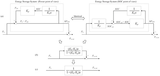
Figure 1.
Block diagram of WT and ESS interface.
2.3. Theorem of ESS Sizing
It is important to note the following guideline for sizing ESS with the proposed method. In case SOC is allocated to the WT rating and the time constant in (11) is determined, the capacity of the ESS can be calculated as shown in (16), which is derived from (6), (7) and (11).
When the WT rating and the time constant are selected, the size of the ESS can be determined using (16), which is also necessary to decide how much the energy the ESS is targeting to use, and it is necessary to determine the range of the SOC to calculate the required capacity of the ESS. The accurate calculation of the ESS size for WT is closely related to the energy usage and the expense of ESS. This equation, which mathematically finds a suitable ESS size for WT, is one of the advantages of this methodology.
3. ESS Integration
3.1. ESS Integration on Renewable Energy
Much research has been conducted on the adverse impacts caused by the fluctuation of wind power, when wind power is connected to the power system [1,14]. However, there have also been several studies in which the wind power fluctuation is reduced; in this case, the grid frequency would have less deviation and becomes more stable. Figure 2 shows a conceptual illustration of a renewable energy-ESS integrated system and the linkage of wind and ESS to the power system. Figure 3 shows a block diagram of this integrated system connected to the power system, which operates with AGC. The block diagram in right side indicates the ideal and aggregated generator operating with Governor and AGC and that in left side explained in Figure 1 and (16) indicates the interface of WT and ESS, which is part of the electrical power (). Practically, additional consideration should be examined such as generator turbine, SCADA system, measurement devices, and other types of communication devices for the application.
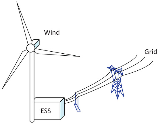
Figure 2.
A wind and ESS integration on power grid.
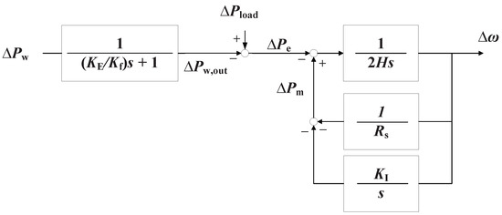
Figure 3.
Block diagram of the wind and ESS integration on power systems.
Table 1 shows the conditions of the case study to compare different examples. Case 1 exhibits a longer time constant, because the ESS capacity is larger than that of others. In Case 2, the ESS capacity is smaller than 5 MW, which exhibits a shorter time constant. In Case 3, the capacity of ESS is the same as that of Case 2 (5 MW); however, the use range of SOC is only 50%, which implies that the range of available energy becomes half; thus, the time constant is reduced.

Table 1.
Case Study for WT and ESS Interface.
3.2. Analysis Using Transfer Functions for ESS Integration
The Bode plot of (15) and Figure 1c can be expressed as shown in Figure 4, implying that ESS is responsible for the high-frequency band of the power generated from the wind power () for sending the low-frequency band output () to the network. In Figure 4, Case 1 exhibits a relatively low cut-off frequency, because the ESS is responsible for a wider band in high-frequency side. In Case 2, the cut-off frequency increases slightly, which implies that the high-frequency band covered by the ESS decreases. In Case 3, the SOC usage range covered by the ESS decreases and the cut-off frequency is further increased as the higher frequency band is reduced, where the ESS is in charge.
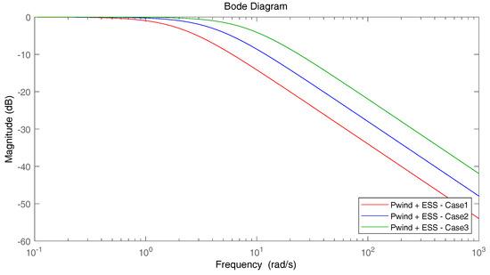
Figure 4.
Bode plot of wind output with ESS from the original wind power.
The Bode plot to observe the effect of wind power on the grid frequency was introduced in a previous study [3], which included generators performing AGC operation for frequency control in the power system. If the WT is interfaced with the ESS using the proposed method for power system integration, the transfer function can be expressed as shown in Figure 3. In this case, the wind and ESS power () is generated with the low-pass filtered form instead of the originally generated wind power, As low-pass filtered power flows into the power system, this transfer function should be combined with the conventional block diagram as shown in Figure 3.
In Figure 5, for the case in which the wind power without ESS affects the power system, the magnitude of the Bode plot is shaped as shown by the black line, where the frequency band with a high magnitude is relatively more affected and the frequency band with a low magnitude is less influenced by wind power. In Case 1, as ESS is responsible for the higher frequency band, the magnitude in high-frequency band is reduced by ESS compared to that of Case 0. The high-frequency band in Case 2 is extended, thus coverage of ESS in high-frequency band is further reduced, since the size of the ESS is reduced in Table 1. In Case 3, the ESS covers a lower bandwidth and the WT power fluctuation has relatively more impact on the grid frequency.
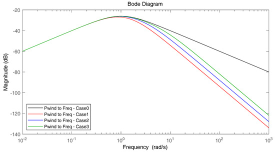
Figure 5.
Bode plot showing impact of renewable energy on power system—Input: wind power, Output: Grid frequency.
3.3. Result of WT-ESS Integration
In Figure 6a, the output power from the interfaced WT and ESS () is comparable to the original WT power in Case 0 in Figure 6a and the ESS power in Figure 6b. In Case 1, the ESS capacity is relatively large according to Table 1, output of the WT + ESS () is the smoothest, as the ESS operates with the highest charge/discharge rate compared to other cases in order to cover a higher frequency band. In Case 2, the output power and the charge/discharge of the ESS is between that of Cases 1 and 3, as the low-pass filtered power has a lower time constant than that in Case 1 and a higher time constant than that in Case 3, due to the smaller size of the ESS than Case 1. In Case 3, the WT + ESS () is characterized by the lowest time constant due to the least compensation from ESS. It also presents the lowest charge/discharge power from ESS because of low energy usage in ESS.
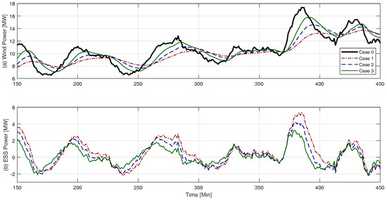
Figure 6.
Power-smoothing output: (a) Wind power, (b) ESS power.
3.4. Grid Frequency
According to the transfer function in Figure 3, the grid frequency fluctuates depending on the wind variability. In Figure 5, as the larger size of ESS is responsible for the higher frequency band, the compensated wind power () would have lesser impact on the grid frequency, resulting in less frequency fluctuation. As shown in Figure 7, without ESS, the frequency will fluctuate significantly as in Case 0. If a large capacity ESS is interfaced with WT, the grid frequency will experience less fluctuation as shown in Case 1. In Case 2, the grid frequency fluctuates less, as the ESS capacity and compensation are reduced. The grid frequency in Case 3 is less fluctuating than that in Case 0 due to ESS compensation, although it has more fluctuation than Case 2 or 3.
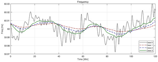
Figure 7.
Grid frequency variation due to the WT power.
4. Time-Domain and Power-Spectrum Analysis
4.1. Case 1
4.1.1. Time-Domain Analysis for Wind Power and SOC
In the case studies, the wind turbine rating () is determined as 20 MW, and the available SOC is assigned as 1 () in pu. In Case 1, the output power () to the grid is smoothed due to the interface of ESS on WT, which has variability. The output power () is identical to , and has the same tendency as that of SOC following the SOC reference, which is proportional to the WT generation in (12). In other words, the fluctuation of wind power () leads the fluctuation of SOC reference (SOCref) in (12). As a result, the output power () is highly identical to the power offset () as explained in (14) and (15), which is proportional to the actual SOC. Conclusively, the output power () is filtered from the original WT power (), which has the same shape as that of the relation between SOC and SOC reference in Figure 8.
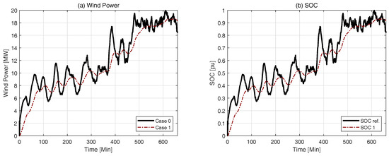
Figure 8.
Wind power and SOC change in Case 1: (a) Wind power, (b) SOC.
4.1.2. Analysis Using Power Spectral Density
In this analysis, we observe which frequency band is compensated by the ESS and how much output power flows to the grid, by using power spectral density. In Case 1, the cut-off frequency is reduced as shown in Table 1, and ESS is responsible for wider compensation on high-frequency band in Figure 9. Consequently, the output power () in low-frequency band is almost similar to the original wind power flowing into the grid. Nonetheless the ESS compensation () in the high-frequency band is identical to original wind power.
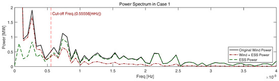
Figure 9.
Power spectral density of WT power and ESS Compensation in Case 1.
4.2. Case 2
4.2.1. Time-Domain Analysis for Wind Power and SOC
In this case, the wind turbine rating () and the available SOC () are equal to the condition in Case 1; however, in Case 2, we select smaller size for the ESS, which is in charge of smaller compensation range in the frequency band compared to Case 1. Therefore, the output power () to the grid is less smooth than that of Case 1 as shown in Figure 10. Figure 10 also shows a similar tendency between the original WT power () with WT + ESS output power and SOC reference with SOC as in Case 1. Thus, Figure 10 shows that the changed size of ESS determines the time constant as presented in Table 1. According to (11), the energy in the ESS () and the feedback coefficient () which are selected from the WT rating () and the usable SOC () naturally determine the coverage of the frequency band against the variability of the WT power.
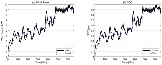
Figure 10.
Wind power and SOC change in Case 2: (a) Wind power, (b) SOC.
4.2.2. Analysis Using Power Spectral Density
Figure 11 indicates that the cut-off frequency of Case 2 increases slightly, which implies that the ESS covers a narrower high-frequency band under the conditions above. Figure 11 also indicates the frequency band of the output power () entering the power grid becomes wider.
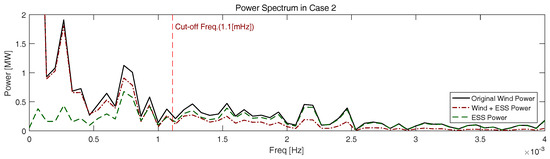
Figure 11.
Power spectral density of WT power and ESS Compensation in Case 2.
4.3. Case 3
4.3.1. Time-Domain Analysis for Wind Power and SOC
In Case 3, the wind turbine rating () and the size of the ESS (E) are equal to the condition in Case 1, but the serviceable SOC () is half of previous condition, 0.5 [pu] (from 0.25 () to 0.75 ()), which changes the feedback coefficient () accordingly. From an energy point of view, this implies that the available energy in ESS is half of that in Case 2. As shown in Figure 12, the range of fluctuation of SOC varies between 0.25 [pu] and 0.75 [pu], following the tendency of the variation of WT generation () and the SOC reference (SOCref) within the designated SOC range () with a high time constant.
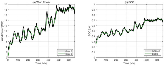
Figure 12.
Wind power and SOC change in Case 3.
4.3.2. Analysis Using Power Spectral Density
In Case 3, the ESS in Case 3 is in charge of the narrowest high-frequency band among all the cases, and has the highest cut-off frequency as shown in Figure 13. From this figure, we can find a high similarity between the original WT power () and the output power () in the frequency band lower than the cut-off frequency, which means that the ESS takes responsibility only in the very high-frequency region of the power spectrum and let low-frequency band of wind power flow into the power system.
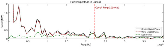
Figure 13.
Power spectral density of WT power and ESS Compensation in Case 3: (a) Wind power, (b) SOC.
5. Conclusions
In this paper, we propose a method of power-smoothing through energy feedback from ESS to reduce the variation of wind power generation as well as ESS sizing. The theoretical background of this method is expressed using a transfer function for which frequency analysis is conducted using Bode plots. Case studies demonstrate the efficacy of the proposed approach by comparing the wind turbine generation with the output power flowing into the system and the SOC reference with the SOC as well. A practical method for sizing the ESS is also proposed based on the SOC range and time constant; furthermore, we also propose a technique for determining the proper time constant for power-smoothing from the information of SOC range and ESS capacity. Time-domain simulations show that the ESS helps reduce fluctuations by performing low-pass filtering with the calculated time constant. Power spectral analysis further clarifies the frequency band where the ESS performs in delivering the power from wind to the grid. The method can also be applied for determining the serviceable SOC range and ESS coverage frequency based on the grid operating conditions.
Author Contributions
J.W.S. conceived the original idea for methodology, and carried out the work for simulation, analysis, visualization, validation, original draft writing, and investigation; H.K. supported the work for investigation, original draft preparation, review, and editing; K.H. supervised this research including project administration, funding acquisition, and methodology development as well as review and editing.
Funding
This research was supported by Basic Science Research Program through the National Research Foundation of Korea (NRF) funded by the Ministry of Education, Science and Technology (grant number 2018R1D1A1A09083054). This work was supported by “Human Resources Program in Energy Technology” of the Korea Institute of Energy Technology Evaluation and Planning (KETEP), granted financial resource from the Ministry of Trade, Industry & Energy, Republic of Korea (No.20194030202420).
Conflicts of Interest
The authors declare no conflict of interest.
References
- Cho, Y.; Shim, J.W.; Kim, S.; Min, S.W.; Hur, K. Enhanced frequency regulation service using Hybrid Energy Storage System against increasing power-load variability. In Proceedings of the 2013 IEEE Power Energy Society General Meeting, Vancouver, BC, Canada, 21–25 July 2013; pp. 1–5. [Google Scholar] [CrossRef]
- Shim, J.W.; Verbič, G.; Hur, K.; Hill, D.J. Impact analysis of variable generation on small signal stability. In Proceedings of the 2014 Australasian Universities Power Engineering Conference (AUPEC), Perth, Australia, 28 September–1 October 2014; pp. 1–6. [Google Scholar] [CrossRef]
- Shim, J.W.; Verbič, G.; Zhang, N.; Hur, K. Harmonious integration of faster-acting energy storage systems into frequency control reserves in power grid with high renewable generation. IEEE Trans. Power Syst. 2018, 33, 6193–6205. [Google Scholar] [CrossRef]
- Jabir, M.; Azil Illias, H.; Raza, S.; Mokhlis, H. Intermittent smoothing approaches for wind power output: A review. Energies 2017, 10, 1572. [Google Scholar] [CrossRef]
- Wang-Hansen, M.; Josefsson, R.; Mehmedovic, H. Frequency controlling wind power modeling of control strategies. IEEE Trans. Sustain. Energy 2013, 4, 954–959. [Google Scholar] [CrossRef]
- Zhou, Z.; Scuiller, F.; Charpentier, J.F.; Benbouzid, M.E.H.; Tang, T. Power smoothing control in a grid-connected marine current turbine system for compensating swell effect. IEEE Trans. Sustain. Energy 2013, 4, 816–826. [Google Scholar] [CrossRef]
- Meng, H.; Yang, T.; Liu, J.Z.; Lin, Z. A flexible maximum power point tracking control strategy considering both conversion efficiency and power fluctuation for large-inertia wind turbines. Energies 2017, 10, 939. [Google Scholar] [CrossRef]
- Marcos, J.; de la Parra, I.; Garcia, M.; Marroyo, L. Control strategies to smooth short-term power fluctuations in large photovoltaic plants using battery storage systems. Energies 2014, 7, 6593–6619. [Google Scholar] [CrossRef]
- Huang, H.; Mao, C.; Lu, J.; Wang, D. Electronic power transformer control strategy in wind energy conversion systems for low voltage ride-through capability enhancement of directly driven wind turbines with permanent magnet synchronous generators (D-PMSGs). Energies 2014, 7, 7330–7347. [Google Scholar] [CrossRef]
- Lee, H.; Hwang, M.; Muljadi, E.; Sørensen, P.; Kang, Y.C. Power-smoothing scheme of a DFIG using the adaptive gain depending on the rotor speed and frequency deviation. Energies 2017, 10, 555. [Google Scholar] [CrossRef]
- Abedini, M.; Mandic, G.; Nasiri, A. Wind power smoothing using rotor inertia aimed at reducing grid susceptibility. Int. J. Power Electron. 2008, 1, 1445–1451. [Google Scholar] [CrossRef]
- Zhao, X.; Yan, Z.; Xue, Y.; Zhang, X.P. Wind power smoothing by controlling the inertial energy of turbines with optimized energy yield. IEEE Access 2017, 5, 23374–23382. [Google Scholar] [CrossRef]
- Liao, S.; Xu, J.; Sun, Y.; Bao, Y.; Tang, B. Control of energy-intensive load for power smoothing in wind power plants. IEEE Trans. Power Syst. 2018, 33, 6142–6154. [Google Scholar] [CrossRef]
- Shim, J.W.; Cho, Y.; Kim, S.; Min, S.W.; Hur, K. Synergistic control of SMES and battery energy storage for enabling dispatchability of renewable energy sources. IEEE Trans. Appl. Superconduct. 2013, 23, 5701205. [Google Scholar] [CrossRef]
- Hasanien, H.M. A set-membership affine projection algorithm-based adaptive-controlled SMES units for wind farms output power smoothing. IEEE Trans. Sustain. Energy 2014, 5, 1226–1233. [Google Scholar] [CrossRef]
- Li, X.; Hui, D.; Lai, X. Battery Energy Storage Station (BESS)-based smoothing control of Photovoltaic (PV) and wind power generation fluctuations. IEEE Trans. Sustain. Energy 2013, 4, 464–473. [Google Scholar] [CrossRef]
- Somayajula, D.; Crow, M.L. An integrated active power filter ultracapacitor design to provide intermittency smoothing and reactive power support to the distribution grid. IEEE Trans. Sustain. Energy 2014, 5, 1116–1125. [Google Scholar] [CrossRef]
- Pegueroles-Queralt, J.; Bianchi, F.D.; Gomis-Bellmunt, O. A power smoothing system based on supercapacitors for renewable distributed generation. IEEE Trans. Ind. Electron. 2015, 62, 343–350. [Google Scholar] [CrossRef]
- Rajapakse, G.; Jayasinghe, S.; Fleming, A.; Negnevitsky, M. Grid integration and power smoothing of an oscillating water column wave energy converter. Energies 2018, 11, 1871. [Google Scholar] [CrossRef]
- Xiong, M.; Gao, F.; Liu, K.; Chen, S.; Dong, J. Optimal real-time scheduling for hybrid energy storage systems and wind farms based on model predictive control. Energies 2015, 8, 8020–8051. [Google Scholar] [CrossRef]
- Yun, P.; Ren, Y.; Xue, Y. Energy-storage optimization strategy for reducing wind power fluctuation via Markov prediction and PSO method. Energies 2018, 11, 3393. [Google Scholar] [CrossRef]
- Han, X.; Chen, F.; Cui, X.; Li, Y.; Li, X. A power smoothing control strategy and optimized allocation of battery capacity based on hybrid storage energy technology. Energies 2012, 5, 1593–1612. [Google Scholar] [CrossRef]
- Wang, G.; Ciobotaru, M.; Agelidis, V.G. Power smoothing of large solar PV plant using hybrid energy storage. IEEE Trans. Sustain. Energy 2014, 5, 834–842. [Google Scholar] [CrossRef]
- Chen, J.; Li, J.; Zhang, Y.; Bao, G.; Ge, X.; Li, P. A hierarchical optimal operation strategy of hybrid energy storage system in distribution networks with high photovoltaic penetration. Energies 2018, 11, 389. [Google Scholar] [CrossRef]
© 2019 by the authors. Licensee MDPI, Basel, Switzerland. This article is an open access article distributed under the terms and conditions of the Creative Commons Attribution (CC BY) license (http://creativecommons.org/licenses/by/4.0/).