Blackbox Large-Signal Modeling of Grid-Connected DC-AC Electronic Power Converters

Abstract

Modern electric power distribution systems are progressively integrating electronic power converters. However, the design of electronic-power-converter-based systems is not a straightforward task, as the interactions among the different converters can lead to dynamic degradation or instabilities. In addition, electric power distribution systems are expected to consist of commercial-off-the-shelf converters, which implies limited information about the dynamic behavior of the devices. Large-signal blackbox modeling approaches have been proposed in order to obtain accurate dynamic models of commercial converters that can be used for system-level analyses. However, most of the works are focused on DC-DC converters. In this work, a large-signal blackbox model is proposed to model grid-connected three-phase DC-AC converters. An experimental setup has been used to demonstrate the limitations of small-signal models and the capability of the proposed modeling approach to capture the dynamic behavior of the converter when large perturbations are applied. Finally, the automation of the model identification process is discussed.

1. Introduction

The smart grid is being accepted by all sectors of society as the solution for a transition towards a renewable-sources-based power supply system. The basic idea is to update the power distribution system according to the progress of technology in many different areas such as power electronics, communications systems, computer science, storage systems, etc. A redesign of the power distribution system would facilitate dealing with the strong variability of the renewable sources, the integration of electric vehicles, optimization of power flows, the establishment of an energy market where the consumers become also producers, blackouts, congestion, among many other problems [1,2,3,4].

The integration of Electronic Power Converters (EPCs) is considered as an enabler for the development of the smart grids. These devices have the capability of providing controllability to the system, integrating communication systems, connecting or disconnecting the different elements of the system, or providing dynamic decoupling allowing the integration of the different elements into the microgrid and the different microgrids among them. This characteristic is very important because a microgrid can be seen as a single element by the rest of the system and, therefore, the dynamic analysis can be performed in a hierarchical way [5].

The dynamic assessment of microgrids is not a straightforward task. This kind of systems is characterized by a high variability coming from the dependency of the power delivered by the energy sources with the weather conditions, the state of charge of the batteries, the presence or not of the grid, and the variable load consumption [6]. This variability leads the converters to work in a wide range of operating conditions, which can compromise the accuracy of small-signal models.

Furthermore, the use of commercial-off-the-shelf (COTS) converters is very suitable for this kind of application in order to decrease the cost of the system and the time-to-market. However, the price to pay by the system designer is that the manufacturers are not expected to provide enough details about the behavior of the EPCs due to confidentiality issues. Therefore, a detailed electrical model of these devices would not be available in general.

The capability of performing simulations of the dynamic behavior of the system is considered of great importance. It is well-known that the interconnection of individually stable EPCs can lead to dynamic degraded behaviors or instabilities. Consequently, the simulation of the system can provide the designers with tools to check the compatibility of the system with standards, design external filters to avoid possible interactions, design protection systems, or assess the compatibility of a new converter with an existing electric power distribution architecture.

In the literature, blackbox models have been proposed in order to deal with the lack of information about the EPCs. The approach consists of applying identification methods in order to obtain a behavioral model able to reproduce the behavior of the devices. Most of the publications related to this topic are focused on DC-DC converters. The different modeling approaches can be classified in linear, static nonlinear, and dynamic nonlinear models according to the type of behavior that the model is able to reproduce. The linear models are based on two-port structures, where the methodologies to identify the transfer functions have been detailed in the literature both in frequency domain [7,8] and in time domain [9]. These models are able to reproduce the average dynamic behavior of any converter around an operating point. Other approaches are focused on predicting the electro-magnetic interferences of the devices [10,11]. The static nonlinear approaches are based on Wiener-Hammerstein structures, which is a block structure. The nonlinearities are included in a static block, often using look-up tables, whereas the dynamic behavior is represented by a linear dynamic block [12,13,14,15,16]. Finally, the dynamic nonlinear models are based on a polytopic approach, where local models around different equilibrium points are integrated in a nonlinear structure [17,18,19,20,21]. The focus of these models is on the small and large signal behavior of the converters under normal operation, short-circuit fault models [22,23,24] are out of the scope of this work.

The blackbox modeling techniques can be applied to AC systems by considering the dq framework, which is equivalent to a DC system. Nevertheless, the number of transfer functions increases considerably due to the partition of the AC variables in the components of the d and q axes. In the literature, only a few examples have been studied regarding DC-AC EPCs. Therefore, it is considered that more effort should be made in the analysis of this type of systems.

The DC-AC converters are very relevant in microgrids. In DC microgrids it constitutes the most relevant element, as it is the point of connection between the microgrid and the rest of the system. In AC microgrids it would correspond to the interface between the grid and DC elements, becoming a key element in the system behavior. Depending on the needs of the microgrid, they can work in different modes: grid-feeding, grid-supporting, and grid-forming. These strategies, in general, allow them to contribute to the control and stability of the grid, fixing the voltage level and frequency when it is controlled as a voltage source, or injecting active and reactive power when it is controlled as a current source [25]. The main contributions of this manuscript are:

• General large-signal blackbox modeling approach for DC-AC EPCs.
• Methodology to perform the tests and identify the transfer functions of the blackbox model.
• Experimental validation of the proposed large-signal modeling methodology using an actual EPC connected to the grid.

The rest of the paper is organized as follows. A brief review of blackbox modeling techniques is presented in Section 2. In Section 3, a description of the blackbox model of a grid-connected DC-AC converter is given. In Section 4, the experimental setup is described and the performance of the large-signal blackbox model identified is presented. Finally, the conclusions are included in Section 6. A brief description about the Output-Error structure, which has been used for the identification of the transfer functions, is given in Appendix A. Also, the polytopic concept is formally described in Appendix B.

2. Blackbox Modeling

Blackbox modeling refers to a modeling approach in which the designer has only partial or no information about the device under test. This strategy is based on the analysis of the response of the system to specific perturbations and the application of identification techniques. Blackbox modeling is especially useful to analyze the dynamic behavior of systems composed of COTS converters, due to the lack of detailed information about the internal architecture of the EPCs and their control loops.

The literature about blackbox modeling strategies for EPCs has focused mainly on DC-DC converters, where the methodology to identify small-signal models around an operating point of DC-DC converters has been described in detail in [7]. Besides, the approach to decouple the identified model from the impedance of the sources and loads used to perform the identification can be found in [26]. Furthermore, nonlinear structures like the Wiener-Hammerstein approach [14] or the polytopic approach [17] have been also proposed for DC-DC converters. More recently, some new strategies have been proposed: to consider the effect of system-level controllers [19,20,27,28], to improve the performance of the model in case strong nonlinearities are present in the system [29], or the first approach towards a blackbox large-signal stability analysis [30]. A review about blackbox modeling structures for DC-DC converters can be found in [31].

Some of these strategies have been extended to DC-AC EPCs. In [32], the use of the dq frame to apply the methodology proposed for DC-DC converters in the DC-AC counterpart is proposed. Afterward, the analogous strategy to obtain unterminated models is applied to this kind of models in [33]. Furthermore, a detailed description of the tests needed to perform the identification of three-phase Voltage Source Inverters (VSI) is presented in [34]. Finally, a preliminary work to consider the large-signal behavior of grid-connected DC-AC converters with droop control is presented in [35] at simulation level.

However, it is considered that more effort should be made to consolidate and to extend the application of blackbox modeling techniques to three-phase DC-AC converters. In this paper, the modeling approach will be applied in an experimental case and the response of the system will be compared with the model estimation. The model structure and the methodology to perform the necessary tests in order to identify the blackbox model will be described. Furthermore, the extension of the polytopic model to this kind of system is considered in order to capture the large-signal behavior of the converter.

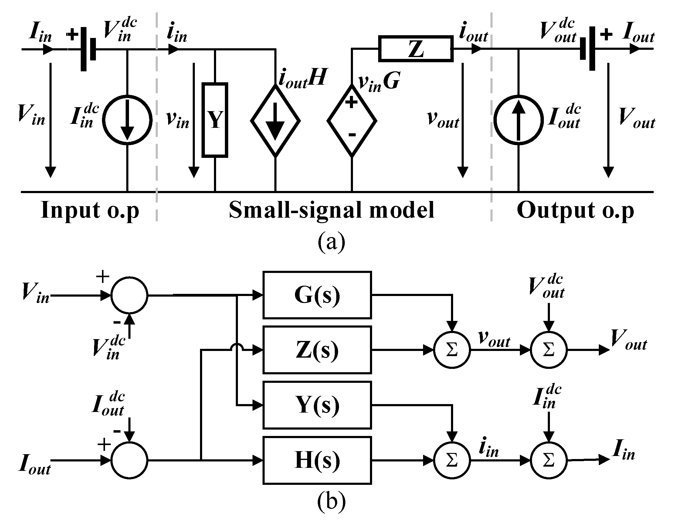
First, the small-signal blackbox modeling strategy for DC-DC EPCs will be briefly introduced. The approach is based on two-port structures. The most common one is the G-parameters model, where the inputs are the input voltage and the output current, whereas the outputs are the input current and the output voltage. The methodology to perform the identification consists of measuring and registering the response of the outputs to small-signal perturbations in one of the inputs, keeping the other one constant. Consequently, two tests are necessary to collect the information needed for the identification. These tests can be performed either in the frequency domain or in the time domain [18]. From the data collected of the input variation and the response of the output variables, a collection of transfer functions that represent the behavior of the converter can be identified. In this case, the Output-Error structure has been applied, a brief description can be found in Appendix A.

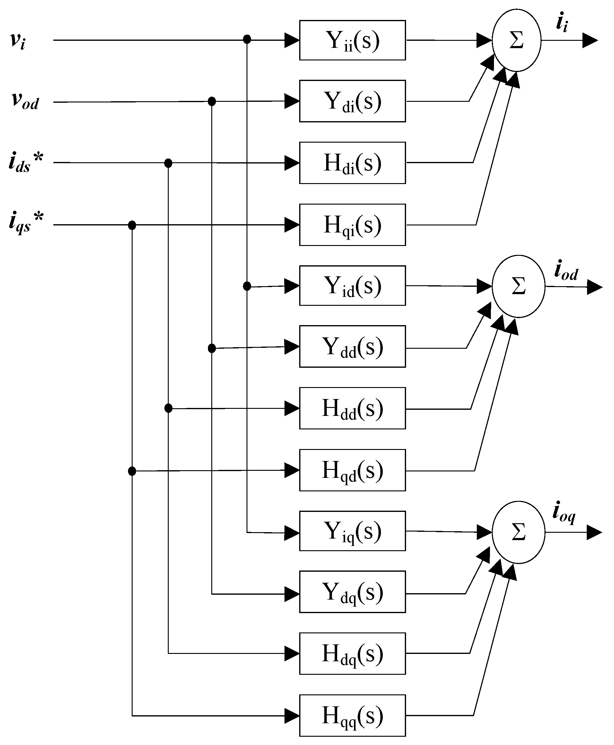
Once the transfer functions have been identified, they must be integrated into a structure where they receive the variations of the input variable from the operating point around which they were identified. Then, their outputs are combined to reproduce the variation of the output variable from the corresponding operating point. In the case of the G-parameters model, the equations that define this structure are

$$\left(\begin{array}{c}{v}_{out}\left(s\right)\\ i_{in}\left(s\right)\end{array}\right)=\left(\begin{array}{cc}G\left(s\right)& -Z\left(s\right)\\ Y\left(s\right)& H\left(s\right)\end{array}\right)\left(\begin{array}{c}{v}_{in}\left(s\right)\\ i_{out}\left(s\right)\end{array}\right),$$

(1)

where $G\left(s\right)$, $Z\left(s\right)$, $Y\left(s\right)$, and $H\left(s\right)$ are the identified transfer functions and $v_{in}\left(s\right)$, $i_{out}\left(s\right)$, $v_{out}\left(s\right)$ and $i_{in}\left(s\right)$ correspond to the variation of the input and output variables around the operating point, as represented in Figure 1.

This linear structure is the base of most of the blackbox models. In case the converter presents an operating point dependent behavior, this model can be adapted to consider its large-signal behavior. The nonlinearities can be classified in static or dynamic. If the nonlinearity is present in the steady-state response and the dynamic behavior can be approximated with a linear model, a Wiener-Hammerstein approach can be implemented. This is a block-based approach which includes nonlinear static functions that set the static operating point of the converter and linear dynamic blocks that account for the transient behavior. This strategy can be implemented with linear networks as in [14], or with a G-parameters structure, where the operating point is variable and dependent on the values of the input variables as in [36]. It should be noticed that with this approach the steady-state of the transfer functions should be unitary, as this value is set by the static nonlinear blocks.

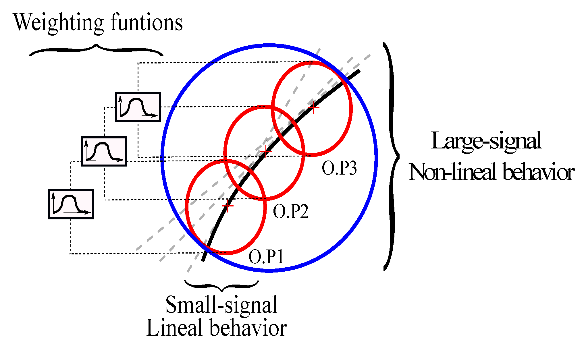
In case the dynamic of the converter is variable depending on the operating point, the polytopic approach can be used. This method consists on identifying small-signal models around different operating points and combining them in a nonlinear structure, where the overall output of the model is a weighted combination of different local models according to the operating point in which the system is working [17]; also in Appendix B, a brief description of the polytopic approach is included.

3. Blackbox Model of Grid-Connected DC-AC Converters

The small-signal models are based on the superposition property, i.e., the response of a linear system to two or more inputs is the sum of the contributions of each input individually. Therefore, in general, a small-signal model can be defined by choosing appropriate input and output variables, which will be related with transfer functions that describe the contribution of each individual input variable in the response of each output variable.

As described before, the AC signals can be considered as DC signals by using the dq framework. Consequently, each AC signal is split into its contribution to the d and q axes. In this work, only balanced systems will be considered, hence the zero sequence is neglected. The converter considered will be controlled as a current source [25], therefore, the input variables will be the input and output voltages, ${\mathit{v}}_{\mathit{in}}$ and ${\mathit{v}}_{\mathit{od}}$ and ${\mathit{v}}_{\mathit{oq}}$, respectively, where the last two variables are the decomposition of the three-phase output voltage in its d and q components. Besides, due to the connection to the grid, the frequency of the grid voltage $\mathit{f}$ can be considered as an input signal in case the effect of the variation of this variable in the response of the system must be considered. Furthermore, taking advantage of the superposition property, also the control references, such as references of active and reactive power, can be considered as inputs of the model. This fact is very appealing to EPCs working in microgrids as it allows taking into account the dynamic effect of variable references in the output variables of the converter, which is a common phenomenon in this kind of applications. In this case, the active and reactive current references are represented as inputs, ${\mathit{i}}_{\mathit{ds}}^{*}$ and ${\mathit{i}}_{\mathit{qs}}^{*}$, respectively. Finally, the controlled and independent variables are set as outputs of the model, namely the input current and the dq components of the output current, ${\mathit{i}}_{\mathit{in}}$ and ${\mathit{i}}_{\mathit{od}}$ and ${\mathit{i}}_{\mathit{oq}}$, respectively. Please note that the same approach can be applied to any other type of converter with any control strategy mutatis mutandis.

Once the input and output variables have been selected, the corresponding transfer functions can be defined.

The small-signal structure will be defined according to the characteristics of the setup under study. The goal is to use the minimum number of transfer functions that are able to reproduce the behavior of the EPC in all the situations considered. It should be noticed that the complexity of the model can grow considerably if every possibility is considered. In particular, the number of transfer functions can be expressed as

$$N_{tf}=N_x{N}_y,$$

(2)

where $N_x$ is the number of input variables and $N_y$ is the number of output variables. In this sense, due to the connection to the grid, it is considered that the frequency variations will be negligible; therefore, this input is not considered in this work. It should be noticed that in an islanded microgrid this would not be the case and this input should be taken into account. Furthermore, the q component of the grid voltage is also neglected. Consequently, with these two simplifications, the number of transfer functions needed to create the small-signal model is reduced from 18 to 12. According to these considerations, the model structure is defined as shown in (3) and its electrical equivalent circuit is depicted in Figure 2.

$$\left(\begin{array}{c}{i}_{in}\left(s\right)\\ i_{od}\left(s\right)\\ i_{oq}\left(s\right)\end{array}\right)=\left(\begin{array}{cccc}{Y}_{ii}\left(s\right)& Y_{di}\left(s\right)& H_{di}\left(s\right)& H_{qi}\left(s\right)\\ Y_{id}\left(s\right)& Y_{dd}\left(s\right)& H_{dd}\left(s\right)& H_{qd}\left(s\right)\\ Y_{iq}\left(s\right)& Y_{dq}\left(s\right)& H_{dq}\left(s\right)& H_{qq}\left(s\right)\end{array}\right)\left(\begin{array}{c}{v}_{in}\left(s\right)\\ v_{od}\left(s\right)\\ i_{ds}^{\ast }\left(s\right)\\ i_{qs}^{\ast }\left(s\right)\end{array}\right).$$

(3)

Finally, it has been mentioned that this work assumes that the converter is balanced. However, in applications such as microgrids, the analysis of unbalanced systems has become an important issue [37,38,39]. In case unbalanced systems should be taken into account, the positive and negative sequences should be considered in the model structure. Also, the zero sequence should be considered in a four-wire system. As a consequence, the number of transfer functions is substantially increased. Those sequences should be represented in the dq framework in order to obtain an equivalent dc system. However, the negative sequence is seen as a sinusoidal signal of double the fundamental frequency in the dq framework of the positive sequence. Consequently, two different dq frameworks should be used for the positive and negative sequences. Afterward, the proper relationship between the dq frameworks and the abc representation must be implemented to add both contributions. Another interesting issue is how to perform the tests in order to introduce perturbations in each input, keeping the rest constant. In some applications, the converter control is designed to detect the positive sequence of the grid-voltage and generate only positive-sequence current, therefore the negative sequence part of the model could be neglected to simplify the model structure. All in all, the application of identification methods for unbalanced systems is considered a very interesting research topic for future work.

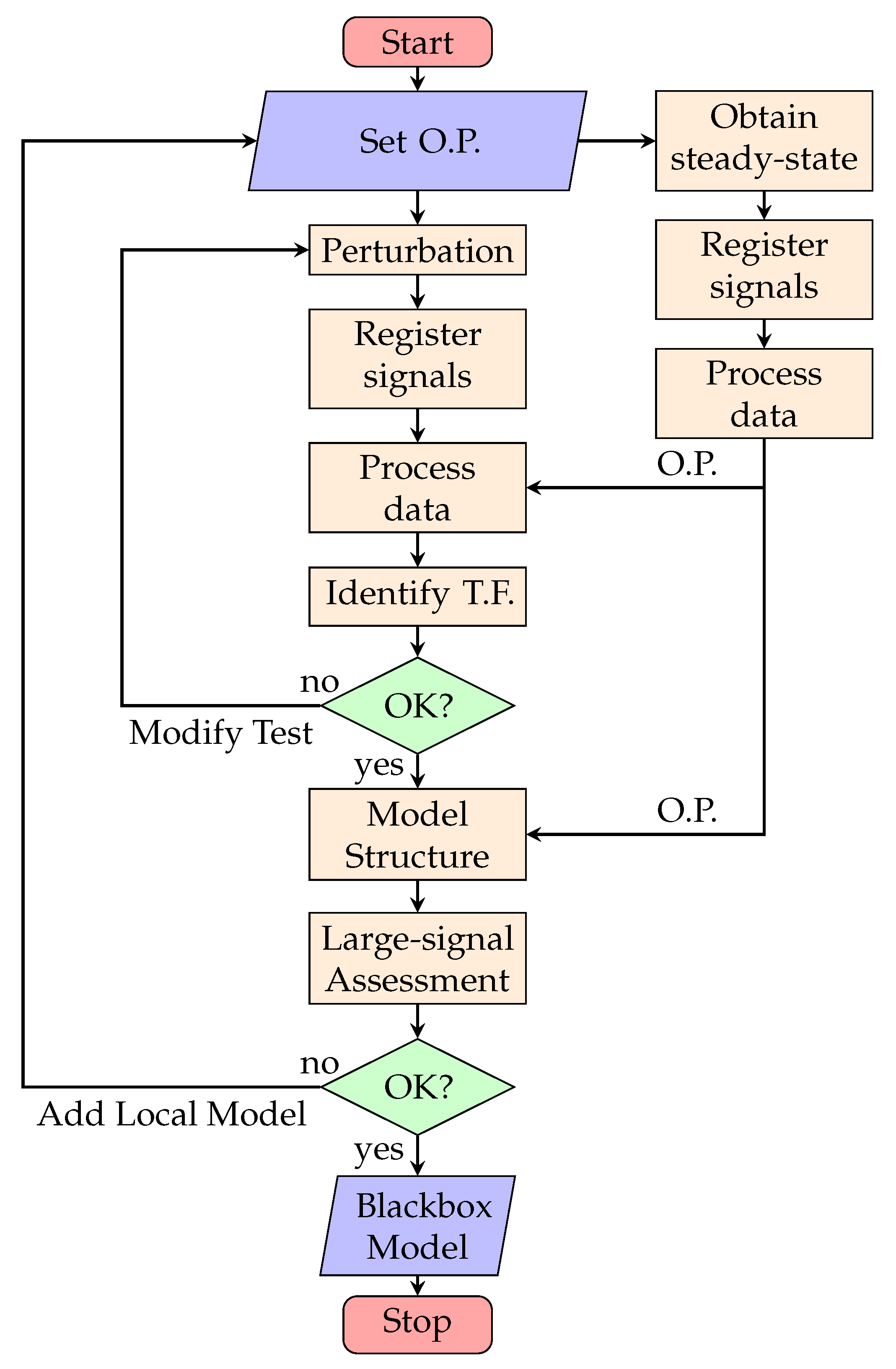
3.1. System Identification

The identification of each transfer function is performed according to the superposition property. It consists of as many tests as the number of input variables. In each test, one of the input variables is perturbed while the rest of them are kept constant. Both the variation of the input variable and the response of the output variables are registered and the transfer functions are identified with this information. In Figure 3 a flowchart of the identification process is depicted.

First, the system is set in a specific operating point by means of the control of the source and the load. Then, a perturbation around this operating point is injected. The perturbation of the input variables can be performed in frequency domain, obtaining bode plots from a frequency analysis, or in time domain varying the inputs with steps. In this work, the latter option has been implemented according to the equipment available. It is worth noticing that the slew rate of the step that is applied to the input variables will define the frequency range that would be possible to identify in the transfer functions, i.e., the higher the slew rate, higher frequencies will be excited and, therefore, the response of the converter at higher frequencies could be identified. In particular, the following condition should be complied with

$$SR>2\pi f{A}_{pk},$$

(4)

where $SR$ is the slew rate of the step, f is the frequency of the sinusoidal signal and $A_{pk}$ is its amplitude. Therefore, if the range of frequencies of interest reaches 1 kHz and an amplitude of the sinusoidal which is much higher than the noise is $0.5$, then the minimum slew rate needed in the step to the input variable would be 3.14 A/ms.

The noise is another important factor when it comes to the identification process. Only the variations which are higher than the noise level will be able to be accounted for. This noise can come from the ripple due to the switching nature of the EPCs or from the measurement equipment itself. Some methods to deal with the noise are: improving the measuring equipment, increasing the level of the input step, and filtering the measured signals. However, the level of the input step must be a trade-off between high enough to produce a response higher than the noise level and low enough to comply with the small-signal condition, i.e., to avoid a nonlinear response. On the other hand, when filtering the measured signals, the cut frequency of the low-pass filter must be well above the range of frequencies of interest, so it does not affect the dynamic of the system.

Once the tests have been performed and the signals have been captured and conditioned, the next step before the transfer function identification is to remove their DC level. Please note that the model structure is a small-signal model, so it represents the variations around an operating point when the input varies around its corresponding operating point. Conceptually, this process is very simple; however, experimentally, it can be more complex due to the presence of noise. In case the noise is considerable, the average value of the signal in the steady state will be subtracted from the signal.

Finally, the filtered signals with zero initial average value are the ones that will be used to identify the transfer functions. In this step, the use of some software is very useful. For instance, in this work, the System Identification Tool of Matlab has been used. For any of the polynomial or transfer functions models available, the information needed, apart from the input and output signals, is the order of the numerator and denominator or the number of zeros and poles. As a result, a fitness percentage, according to the similarity between the output signal and the response of the model, will be obtained. In this part, a trade-off between accuracy and complexity should be made. It also should be noticed that if the order of the model is set too high, it will try to capture the noise of the signal, which will result in undesired behaviors. Therefore, the lowest order that is able to capture the average dynamic response of the system should be selected.

The collection of transfer functions must be integrated in a model structure, in this case the one depicted in Figure 2. At this point, a small-signal model around an operating point has been obtained. The next step would be to assess whether the system presents nonlinearities in its dynamic behavior or not. This assesstment can be performed by comparing the response of the model and the converter under large variations of the input variables. In case the system is accurate for small-signal variations and the accuracy is compromised with large-signal variations, a polytopic approach should be followed. In that case, the same procedure should be performed changing the operating point. Finally, the collection of local models around different operating points would be integrated in a polytopic structure.

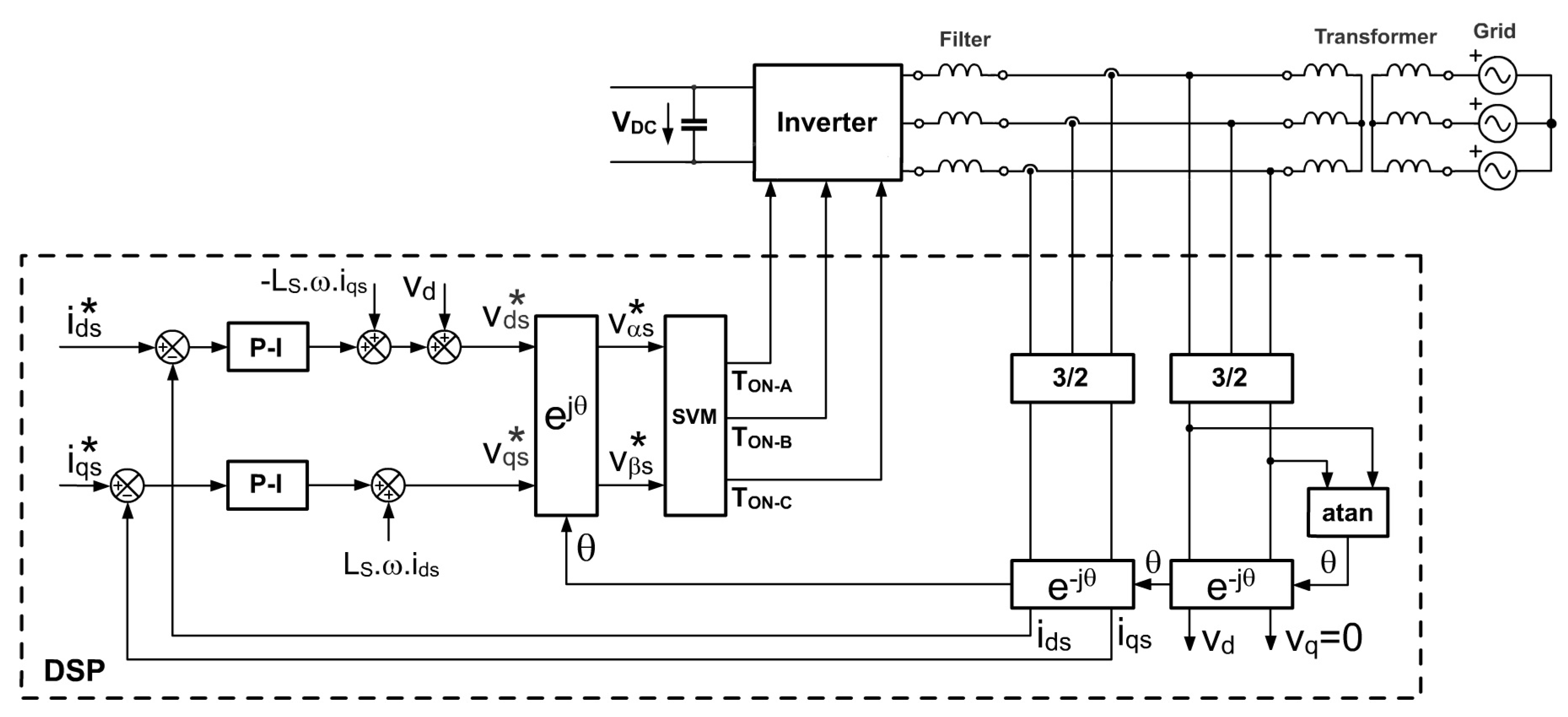
4. Experimental Setup

In this section, the blackbox model of a three-phase DC-AC EPC working as a VSI will be derived. In the following, the characteristics of the hardware implemented will be described, as well as the control system, the identification process, and the comparison between the response of the EPC and the blackbox model estimation.

4.1. System Description

4.1.1. Hardware

The main system comprises a standard electronic power converter made up of six IGBTs and anti-parallel diodes, plus a rectifier to charge the DC link capacitor, a three-phase step-up transformer and filter inductors, Figure 4.

From the control point of view, the system is made up of a dual-core microcontroller connected to four voltage sensors and three current Hall effect sensors.

The microcontroller splits the tasks into two parts: control tasks and communication tasks. The control tasks are carried out by an F28335 core, which switches the IGBTs and takes voltage and current samples at a 5 kHz rate. The communication tasks, carried out by the ARM Cortex M3 core, encompass from sending data to the user interface (connected either through Ethernet or USB) up to taking data from/to the other core through a shared RAM memory.

4.1.2. Control System

The control system programmed in the control core of the Concerto microcontroller is the standard vector control for a converter connected to the grid, Figure 5. Two current loops control the d and q components of the current injected into the grid by means of fast proportional integral (PI) regulators. After adding the corresponding decoupling terms to the PI outputs, the voltage to be generated by the EPC is obtained, expressed in the moving dq reference frame.

Then, the inverse Park transform converts them to the two phases—frame representation with a rotation over an angle. Afterward, the microcontroller calculates the on/off time of every IGBT using a space vector modulator (SVM). As a result, the inverter generates a three-phase voltage that yields the current established by the references ${\mathit{i}}_{\mathit{ds}}^{*}$ and ${\mathit{i}}_{\mathit{qs}}^{*}$.

The list of electrical components used in the successive test is shown in

Table 1. List of devices and electrical components used in the experimental tests.

Device	Model	Ratings
Voltage Source Converter	Semikron SEMISTACK SKS35F B5U	$I_{max}$ = 35 A; $Va{c}_{max}$ = 380 V; $Vd{c}_{max}$ = 750 V; $f_{max}$ = 10 kHz
Dual-core microcontroller	Texas Instruments F28M35x Concerto	150 MHz F28335 + 120 MHz ARM Cortex M3
Step-up transformer	Connection: Y-y 0	Sn = 10 kVA; 400 V/230 V 14.4/25.1 A
Inductances	Laminated iron core	L = 48 mH
DC solid-state relay	CRYDOM LVD75B80	0–80 A; 3–75 VDC
Three-phase solid-state relay	CRYDOM D53TP500	50 A per phase; 48–530 VAC
Resistor bank (2)	Array of resistors	16 $\mathrm{\Omega }$–570 $\mathrm{\Omega }$
Autotransformer (2)	Y-y	400 V adjustable
Oscilloscopes (2)	Two Tektronix TPS2024	20 MHz; 2 GS/s
AC/DC Current Clamps	Fluke i30s	Resolution of 100 mV/A
Voltage sensors	LEM LV15-P	Hall effect; up to 680 V
Grid voltage	Three-phase	100 V rms line to line; 50 Hz

.

4.2. Blackbox Model Identification

In this section, the methodology detailed in Section 3.1 is applied to the particular case described before. According to the model defined in (3), four tests should be performed. Next, the description of the tests is detailed.

4.2.1. $V_{in}$ Step

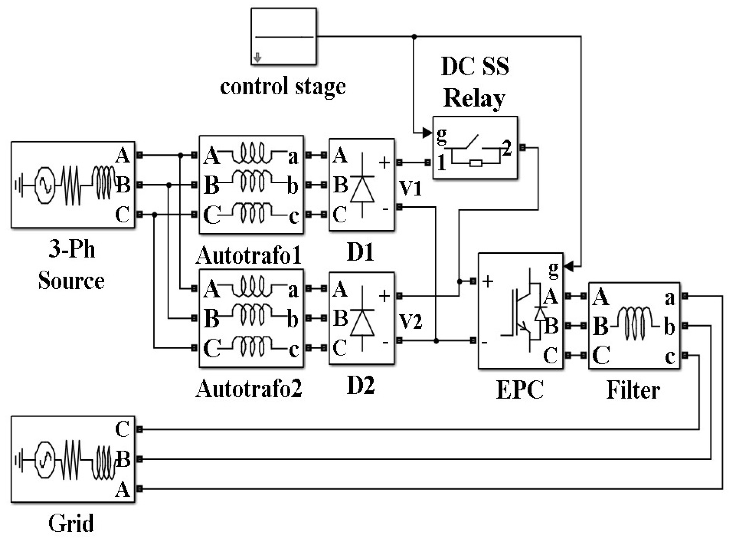
Due to the high capacitance of the voltage sources, in general, a sharp step in the input voltage cannot be performed by changing the voltage reference of these devices. In this case, two voltage sources with different voltage levels have been implemented, where the difference between the two voltages is the desired voltage step. The approach to generating the step is to connect both sources in parallel including a relay in series with the source with a higher voltage level. In this way, when the relay is open, the input voltage will be imposed by the source with a lower voltage level. Alternatively, when the relay is closed, the output diode of the source with a lower voltage value will be reverse biased and the input voltage will be imposed by the source with a high voltage level. With this approach, a suitable slew rate in the voltage variation is obtained. The connection scheme implemented for this test is depicted in Figure 6.

Two autotransformers have been used as voltage sources. The relay was controlled with the same microcontroller used for the control of the converter and the trigger signal was synchronized with the oscilloscopes in order to capture both the input voltage step and the response of the output variables. Finally, the maximum voltage across the relay is limited to 75 V, so this is the value of the maximum step possible with this device.

4.2.2. $V_{od}$ Step

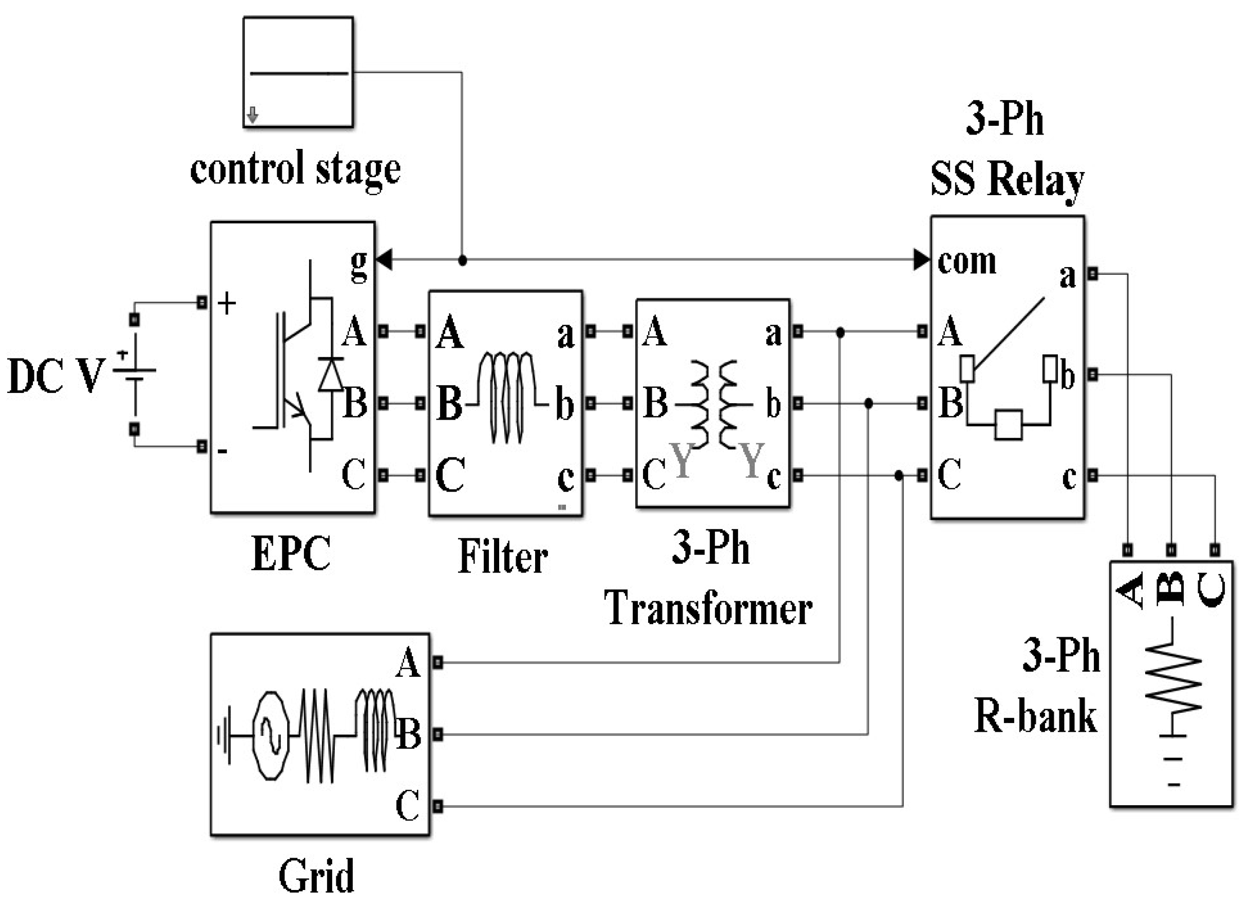
A resistor bank has been used in order to generate a step in the d component of the output voltage. These resistors are connected through a three-phase AC relay, which is managed by the microcontroller and synchronized with the oscilloscopes as in the previous case. The connection of the resistor bank is included between the grid and the three-phase transformer, so, afterward, the unterminated model can be extracted following the methodology detailed in [33]. The connection scheme implemented for this test is depicted in Figure 7.

4.2.3. $I_{ds}^{\ast }$ and $I_{qs}^{\ast }$ Steps

The generation of steps in the variable references is straightforward. A change in the reference of d and q components of the current is programmed in the microcontroller, which is again synchronized with the oscilloscopes in order to capture the response of the output variables.

The direct fitness measurement between the output signal and the model response is not the best metric for this kind of identification process. Instead, the comparison between the average of the output signal and the model response should be used as a figure of merit. Please note that attempting to use a low-pass filter to obtain the average value of the output signal would affect the real dynamic response of the signal, so a more sophisticated noise subtraction method should be implemented, as could be a moving-average filter. On the other hand, if the fitness value is taken as a trustworthy metric and the order of the model is incremented, the model will try to approximate the noise response. Furthermore, if the noise in the input signal is lower than the noise in the output signal, the model considers that a small input produces a high response, which would result in a model that does not represent the system at all. Once the transfer functions have been identified, they can be integrated into the small-signal structure, as depicted in Figure 8.

4.3. Large-Signal Analysis

The blackbox models obtained using this approach are accurate approximations of the EPCs when their behavior is linear or when the range of variations of the input variables is small.

To assess the large-signal behavior of the system, the amplitude of the steps is increased progressively until the model starts to decrease its accuracy. Illustrating this idea, the nonlinear behavior of the converter for different values of the input voltage is studied. In Figure 9, the comparison between the system response and the small-signal model estimation for a step in the input voltage of 30 V is shown when the converter is working in a specific operating point ($I_{od}$ = 3 A, $I_{oq}$ = 0 A, $I_{in}$ = 0 A, $V_{od}$ = 100 V, and $V_{in}$ = 320 V). It can be seen that the performance of the model is very accurate.

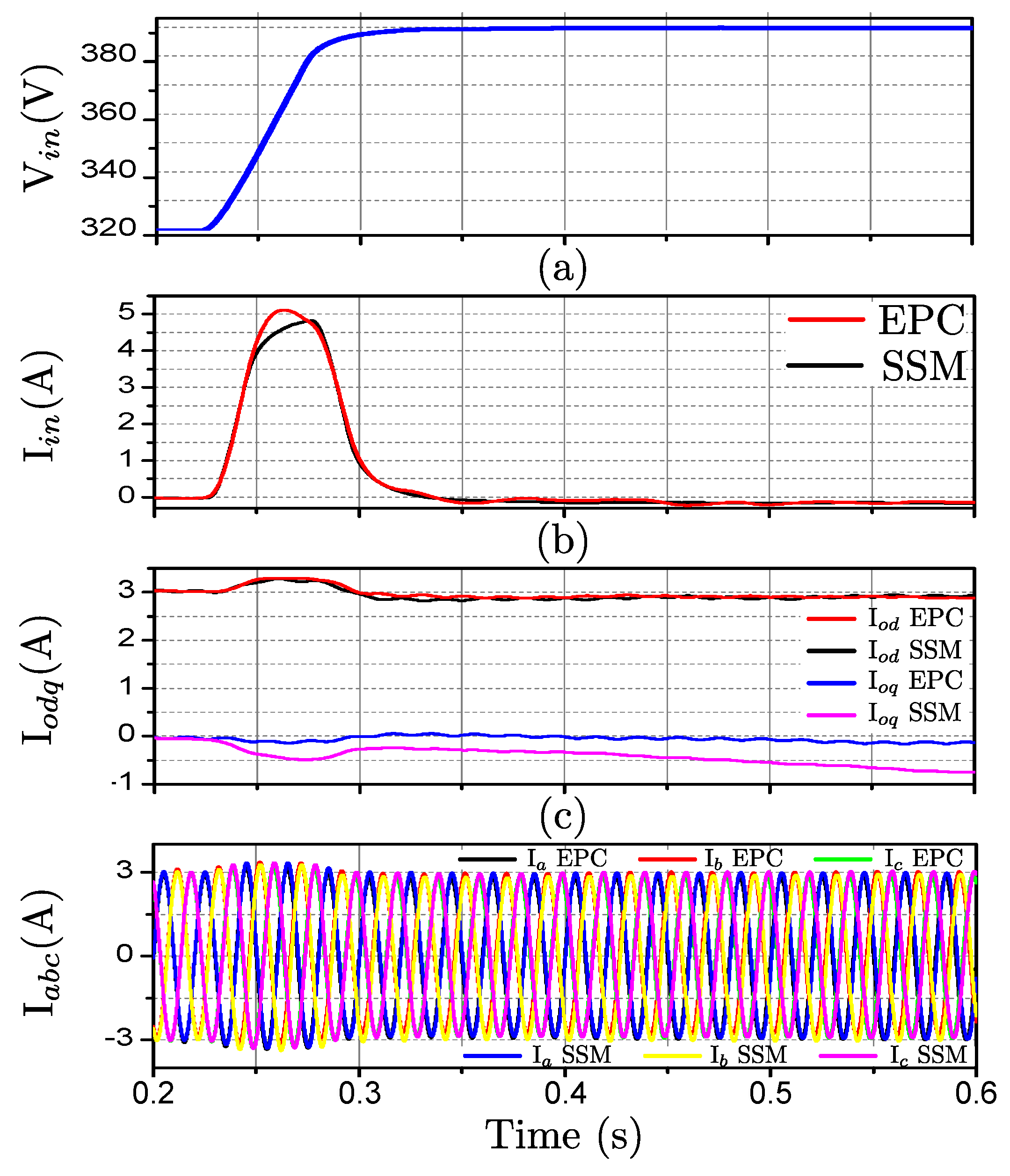
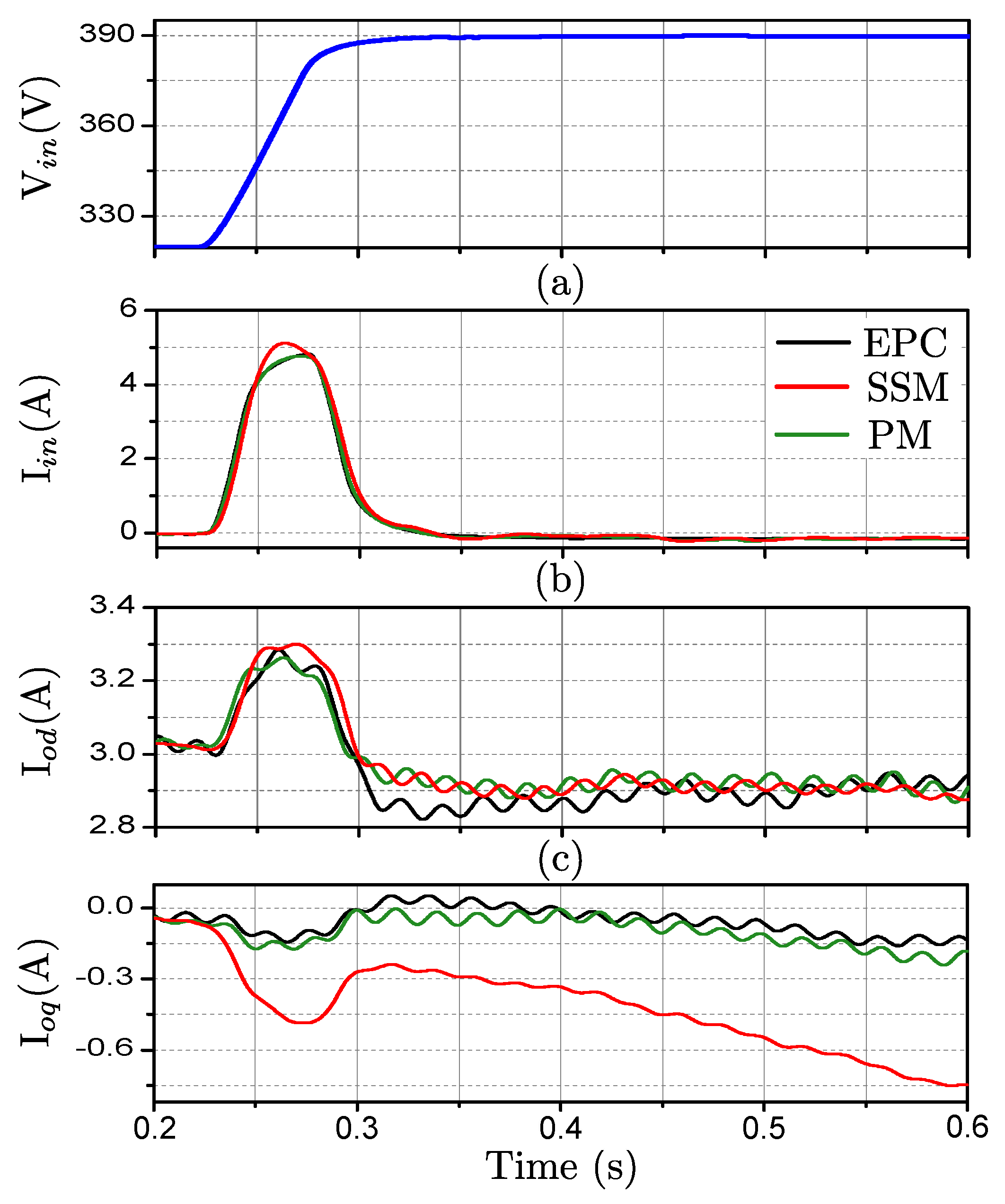
Equivalently, in Figure 10, the comparison between the system response and the small-signal model is shown when the step in the input voltage is increased to 60 V from the same operating point. It can be noticed how the estimation of the model starts to differ from the response of the system in this case.

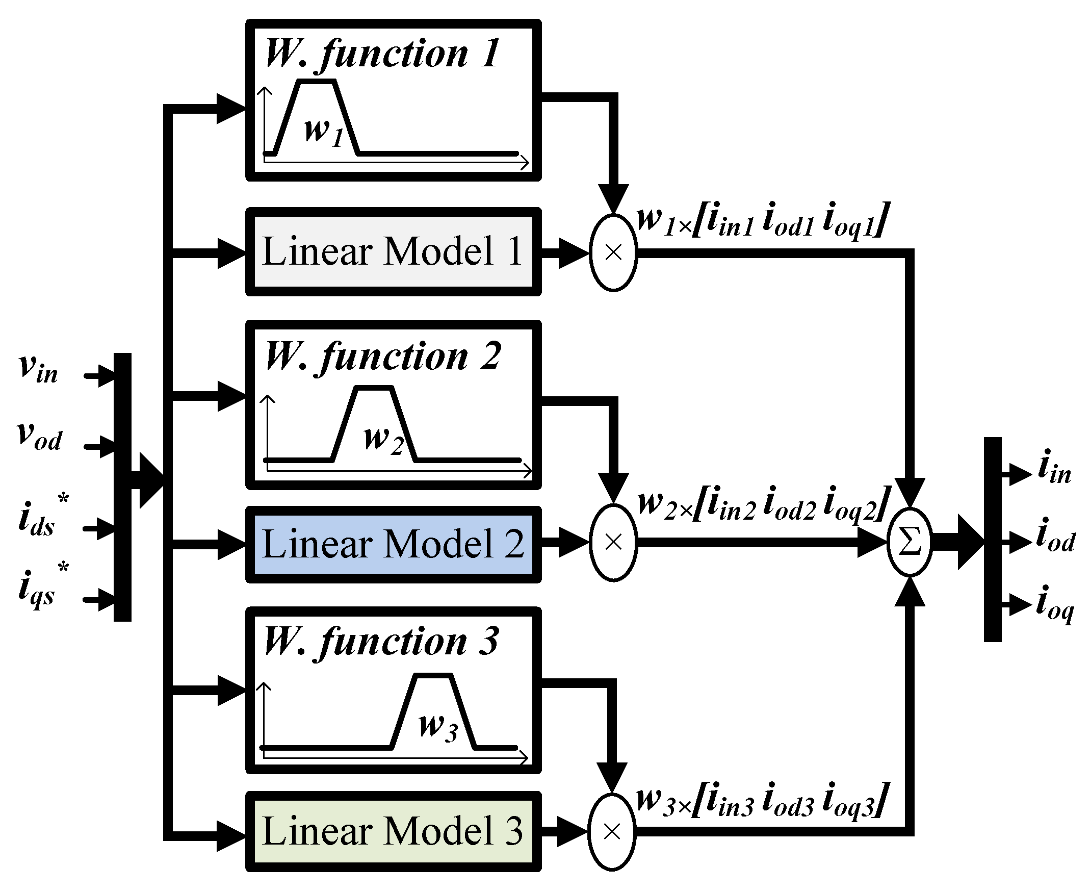
To improve the model accuracy when the operating point is varied in a wide range of values, the polytopic approach is applied. As mentioned in Section 2, this methodology is based on a weighted combination of small-signal models identified around different operating points. This approach has been successfully applied in DC systems [17,19,20,31], and extended to AC EPCs in [35] at simulation level. Therefore, the present work is the first evidence of a polytopic model applied to represent an actual three-phase DC-AC EPC.

The scheme of the polytopic model implemented is depicted in Figure 11. In this case, nine operating points have been selected, which are detailed in

Table 2. Operating point setup and step values.

			Operating Point
Variable	1		2		3
	o.p.	step	o.p.	step	o.p.	step
$V_{DC}$	320 V	30 V	320 V	30 V	320 V	30 V
$V_{L\left(rms\right)}$ ($V_{od}$)	100 V	−8 V	100 V	−8 V	100 V	−8 V
$I_{ds}^{\ast }$	3 A	3 A	6 A	3 A	9 A	3 A
$I_{qs}^{\ast }$	0 A	5 A	0 A	5 A	0 A	5 A
	4		5		6
$V_{DC}$	350 V	30 V	350 V	30 V	350 V	30 V
$V_{L\left(rms\right)}$ ($V_{od}$)	100 V	−8 V	100 V	−8 V	100 V	−8 V
$I_{ds}^{\ast }$	3 A	3 A	6 A	3 A	9 A	3 A
$I_{qs}^{\ast }$	0 A	5 A	0 A	5 A	0 A	5 A
	7		8		9
$V_{DC}$	380 V	20 V	380 V	20 V	380 V	20 V
$V_{L\left(rms\right)}$ ($V_{od}$)	100 V	−8 V	100 V	−8 V	100 V	−8 V
$I_{ds}^{\ast }$	3 A	3 A	6 A	3 A	9 A	3 A
$I_{qs}^{\ast }$	0 A	5 A	0 A	5 A	0 A	5 A

.

This particular selection of operating points has been selected according to the nonlinearities detected experimentally applying steps to the input variables of different amplitudes, as described before; and the expected range of variation of the variables, which is limited by the voltage and current rating of the different devices.

4.4. Experimental Validation

A polytopic model has been assembled using small-signal models identified around the operating points detailed in Table 2. The performance of this model will be compared with the response of the system in the cases where the small-signal model starts to lose accuracy.

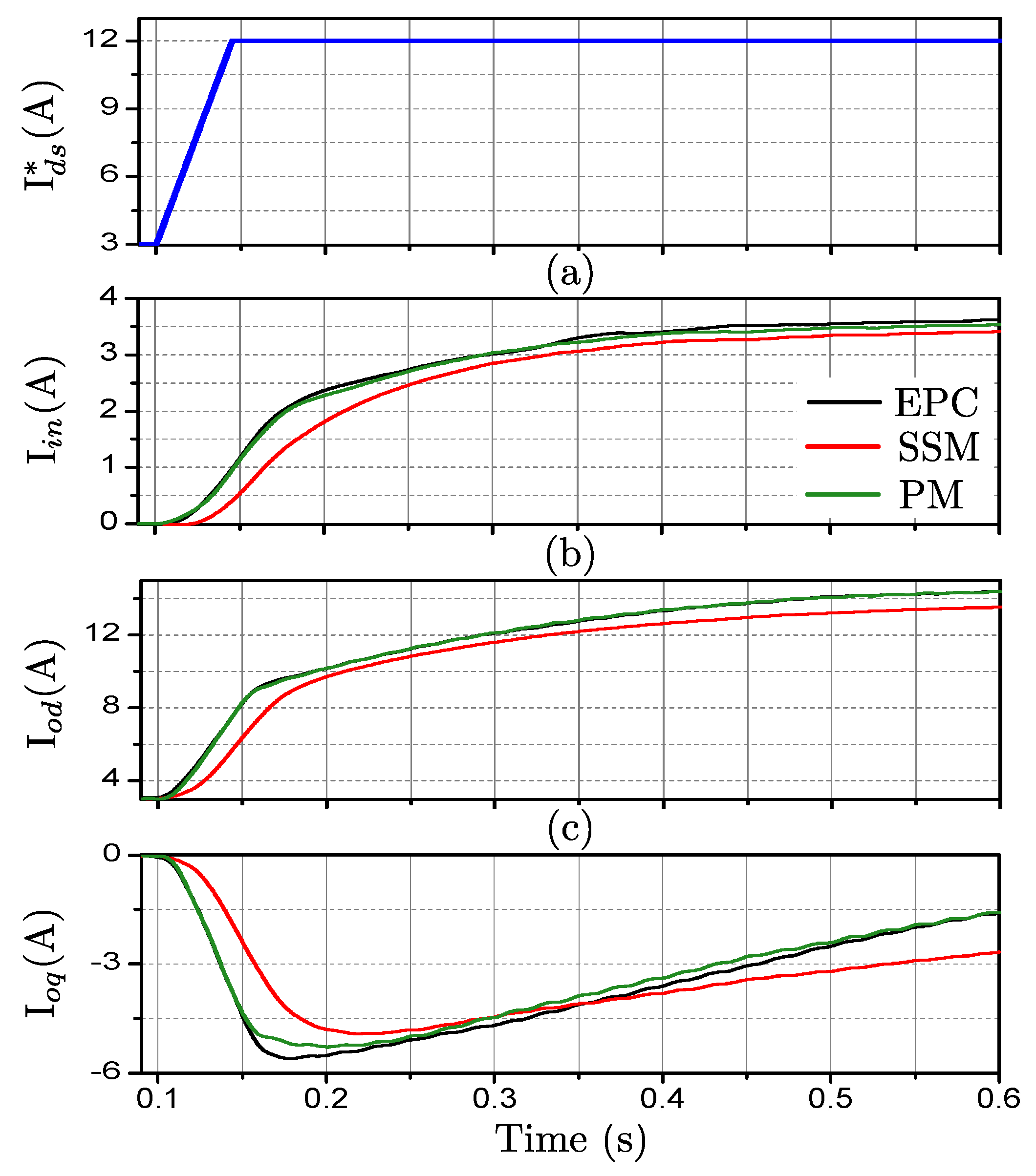
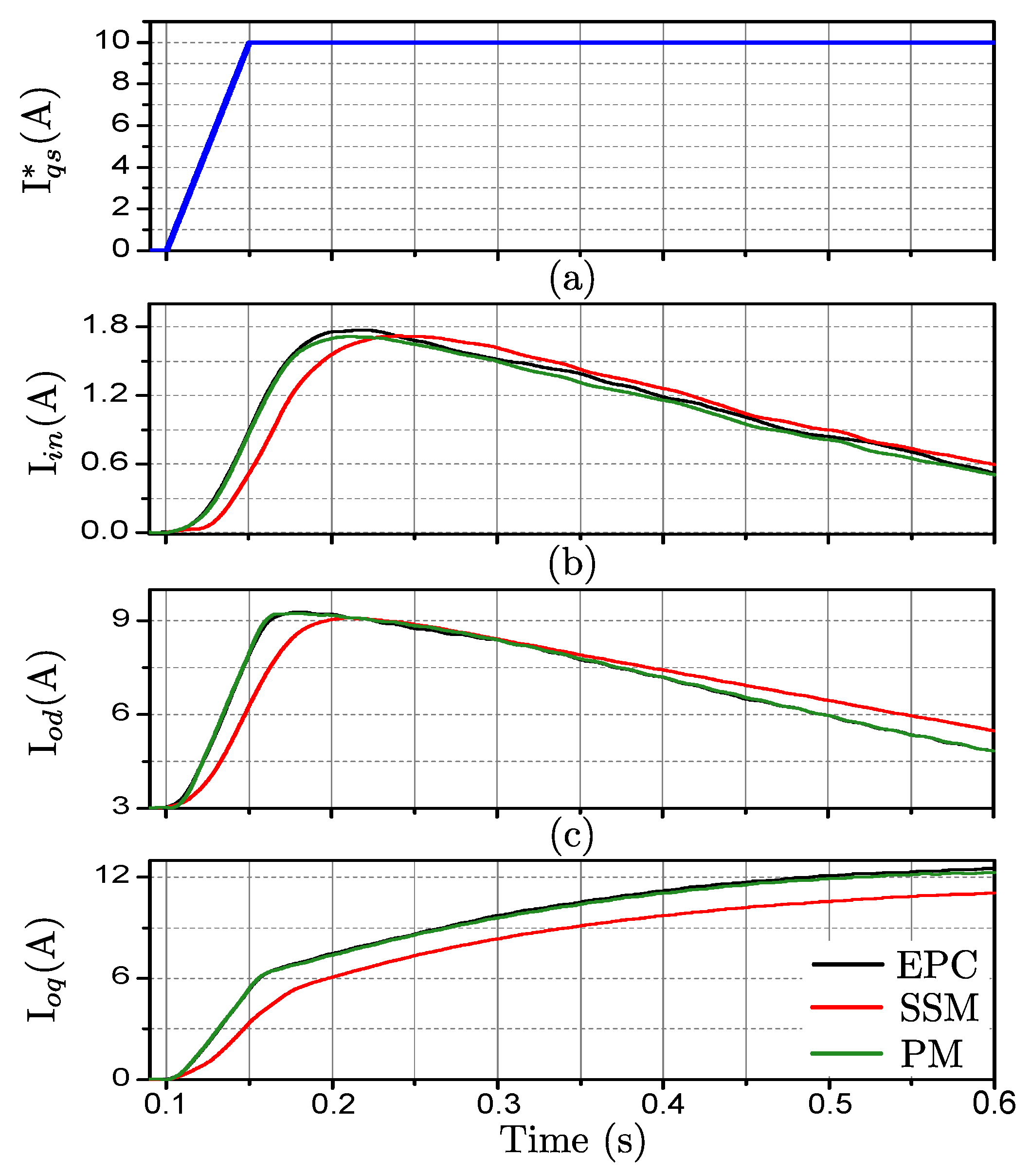
In Figure 12 the polytopic model is compared with the response of the EPC with a step of 60 V in the input voltage. Equivalently, the comparison is shown when the reference of the d component of the output current is increased in 9 A in Figure 13 and when the reference of the q component of the output current is increased in 10 A in Figure 14.

The comparisons show a clear improvement in the estimation of the model compared with the performance of the small-signal model, which validate the proposed modeling approach. The small-signal model was obtained in the initial operating point, before the step. Giving a step large enough in the input signals, the operating point dependent dynamic behavior of the converter is evidenced by the loss of accuracy of the small-signal model. The polytopic model integrates small-signal models around different operating points, therefore by tracking the operating conditions of the model, which are the inputs of the weighting functions, it is able to adapt its dynamic response to reproduce accurately the large-signal behavior of the converter.

The presented results demonstrate that small-signal models are accurate when the operating conditions are close to the operating point where the model was identified. However, after a large step in the input variables, the accuracy of these models is reduced, due to the nonlinearities of the system. The polytopic model is able to account for small and large perturbations, showing a high accuracy in all conditions. Therefore, for applications where high accuracy of the dynamic performance of the system is needed, the increased complexity of the polytopic model, due to its combination of different local models, is justified. Furthermore, this blackbox modeling approach can be extended to inverters with any operation mode, including grid-connected and islanded modes, which is important for the design of AC microgrids.

In the future work, other kind of phenomena that lead to nonlinear responses of the converter will be analyzed. Some interesting examples can be converters with different operation modes, for instance grid-feeding and grid-supporting; unbalanced system; harmonic distortion, etc. All these examples are more complex because they create strong nonlinearities which depend on discrete control actions, or they lead to a more cumbersome model structure, as it is the case of the unbalanced systems.

5. Automation Process

In this paper, it has been demonstrated how the large-signal modeling approaches proposed for DC systems can be applied to their three-phase AC counterparts by using the dq transformation. However, the number of transfer functions needed for this kind of system increases considerably with the number of inputs and operating points considered. Therefore, in order to develop a practical methodology in the industry to simulate DC and AC microgrids, the automation of the identification process would be of great help. It has been shown along the manuscript that the modeling approach is sequential and the procedure is well-defined, therefore, it is considered to be very suitable to be automated. The idea consists in the development of a hardware that is able to follow the flowchart presented in Figure 3 in an automated way, i.e., to set an operating point in the EPC, to perform the perturbations (in time or frequency domain) in the input variables, to register the perturbations and the response of the output variables, to process the measured data, to perform the identification of the transfer functions, and to integrate them in the model structure. Afterward, the system should assess the performance of the model in large-signal conditions and repeat the process for different operating points in order to create the polytopic structure, in case it is needed. The development of hardware able to set the operating point of an EPC and perform steps in the input variables is not an issue, it would be enough to use controllable sources, loads, and switches. In this part, the user should provide some information about the particular EPC under test, as the range of operation of the variables, the definition of inputs and outputs, etc. Also, the registration of the dynamic response of inputs and outputs is not a complex task; however the use of adequate equipment with a high noise rejection is highly advised. As detailed in the paper, a synchronizing signal should be sent to the measuring devices in order to capture the response in the precise moment of the perturbation, which can be in the order of micro or milliseconds. Once the data has been gathered, a suitable filtering process, abc to dq transformations, and the subtraction of the DC bias should be performed. This part is crucial in the identification process as a noisy signal or the presence of a DC bias in the signals can lead to models with very poor accuracy. If the previous steps have been done correctly, the identification part and their integration in the model structure should be straightforward. In case the performance of the small-signal model is not satisfactory, the tests should be repeated, varying the amplitude of the perturbation, which should produce responses higher than the switching ripple and noise level, but keep the small-signal conditions. Also, the filtering process or the DC bias elimination can be modified in order to improve the identification of the model. Please note that, as described in the paper, the presence of noise can make the filtering and DC bias elimination complex. Also, the definition of a suitable figure of merit to select the transfer functions should be made in order to obtain the lowest-order system that is able to reproduce the average behavior of the EPC. Finally, in order to assess the large-signal behavior of the model estimation, it should be compared with the system response in different conditions from where they were identified. In case the EPC shows an operating point dependent dynamic behavior, the process will be repeated for different operating points and the polytopic model can be designed.

6. Conclusions

In this work, the methodology to obtain blackbox models that have been applied to DC systems is extended to their AC counterparts, by transforming the three-phase AC signals into the dq framework. In particular, a grid-connected three-phase DC-AC EPC has been used as a test bench. Details about the small-signal model definition are discussed, as the inclusion of control references, which can be very relevant when system-level controllers are implemented. The identification process, perturbations, signal processing, transfer function identification, and model integration is also discussed in detail. Finally, the suitability and limitations of the blackbox small-signal model obtained are illustrated experimentally.

An important part of this manuscript is concerned with the large-signal analysis of the EPC. The operating point dependent dynamic behavior of the EPC under study is evidenced. It is shown how a small-signal model is very accurate when the amplitude of the perturbation in the input variables is small enough, whereas its performance is deteriorated when the amplitude of the perturbations increases. The design and implementation of the polytopic model for this converter are detailed and its capability to account for the large-signal behavior of an actual inverter is demonstrated.