Simulation of Surfactant Oil Recovery Processes and the Role of Phase Behaviour Parameters


Abstract
:1. Introduction
1.1. Surfactant Flooding
1.2. Aim of this Work
2. Methods
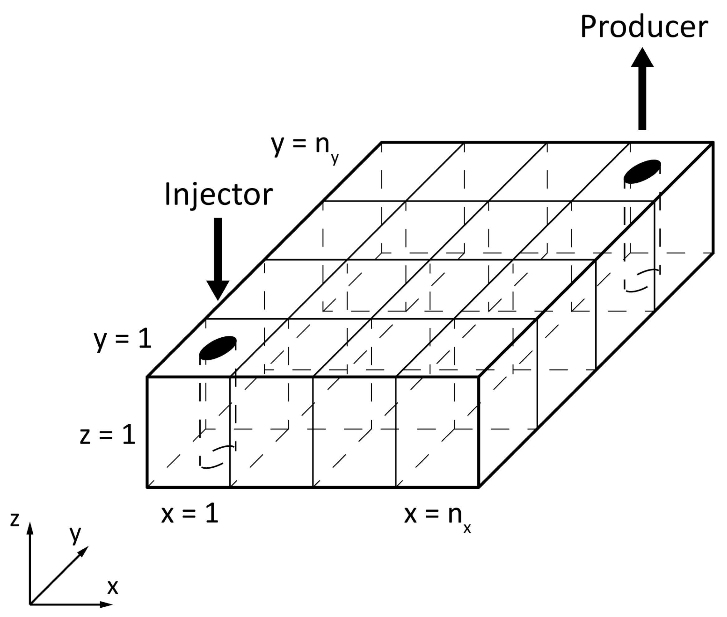
2.1. Physical Model
2.2. Mathematical Model
2.2.1. Discretization of the Partial Differential Equations
2.2.2. Boundary Conditions
2.3. Physical Properties
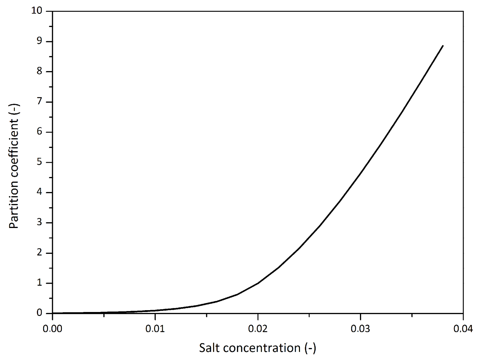
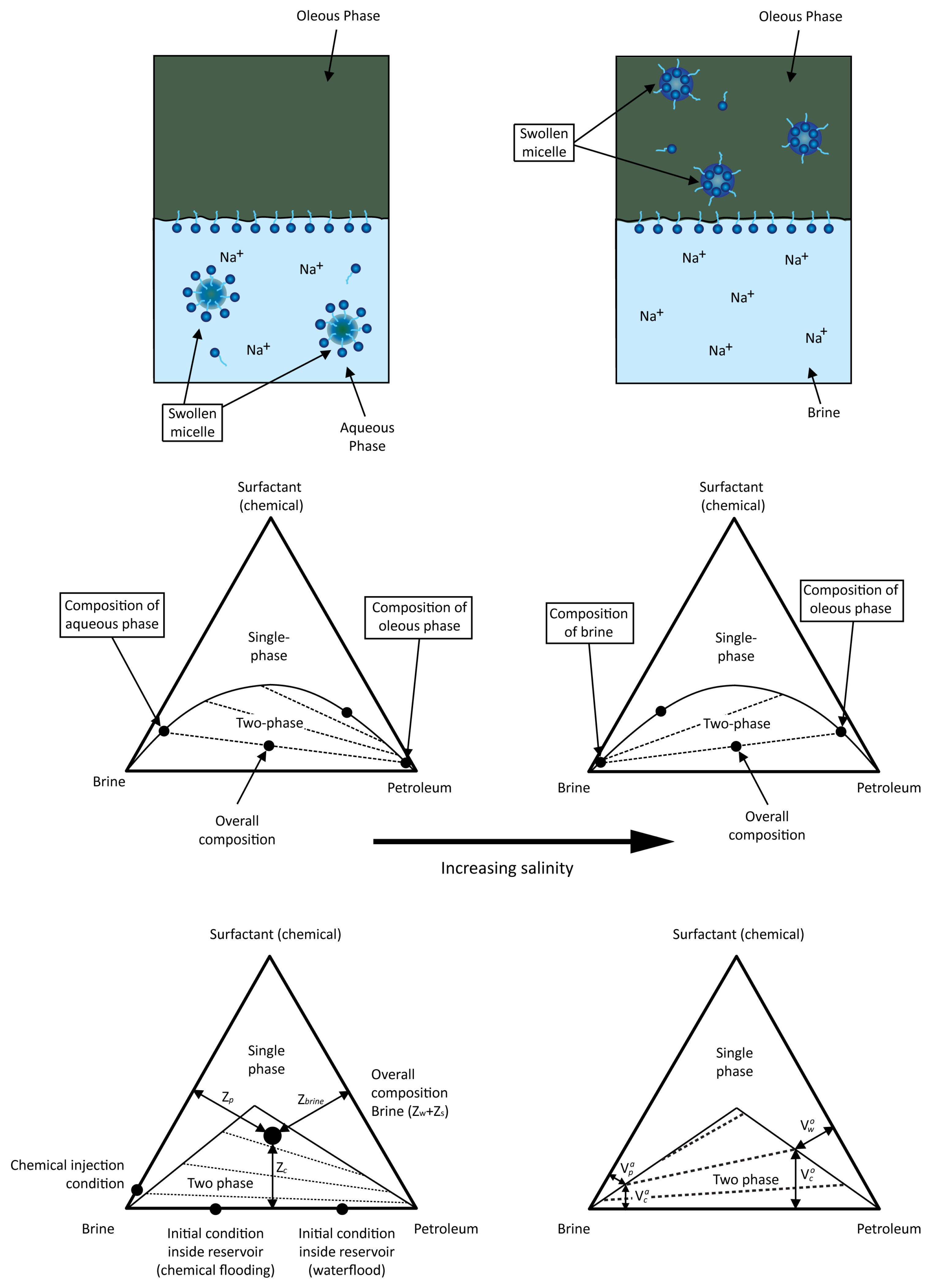
2.3.1. Chemical Component Partition
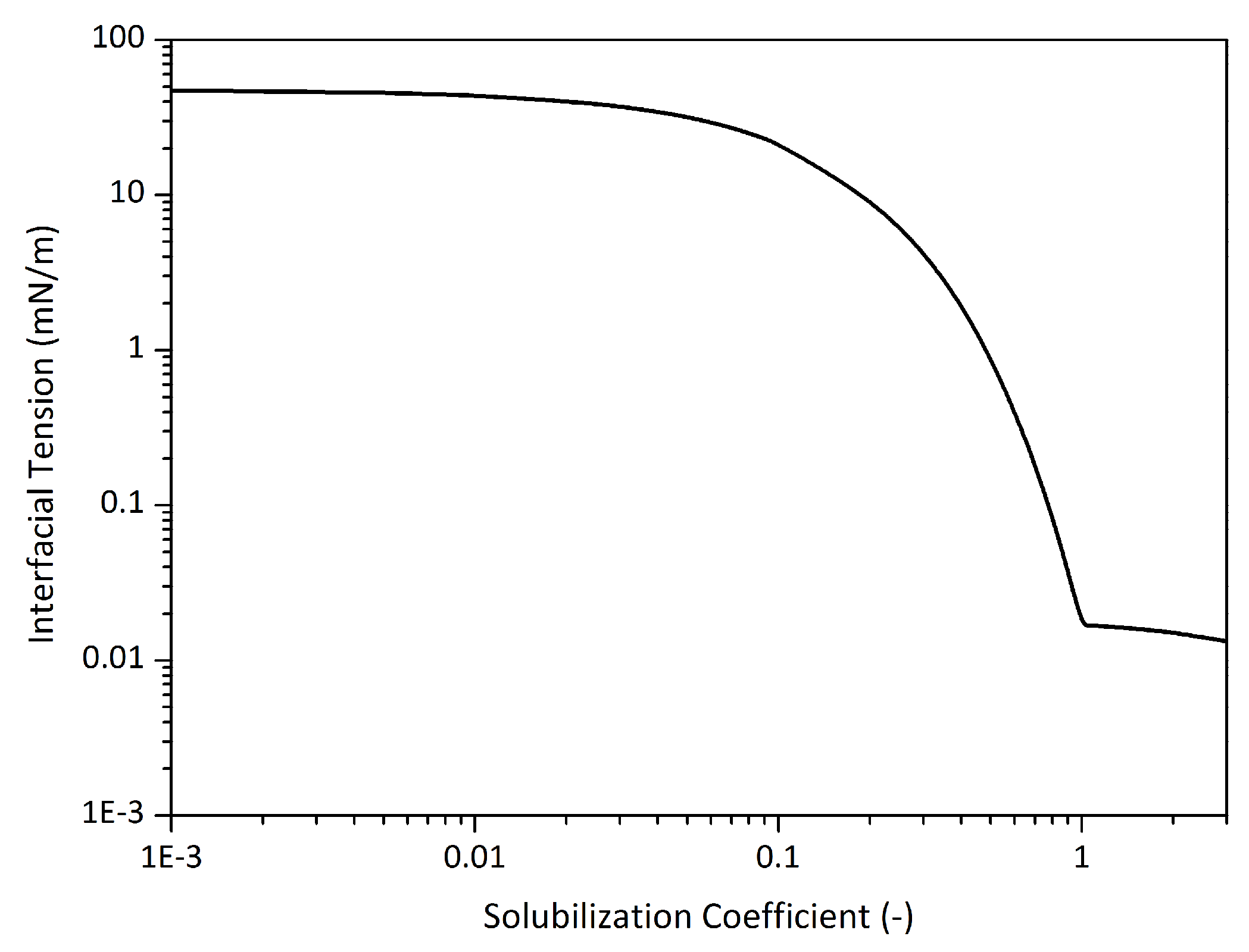
2.3.2. Interfacial Tension
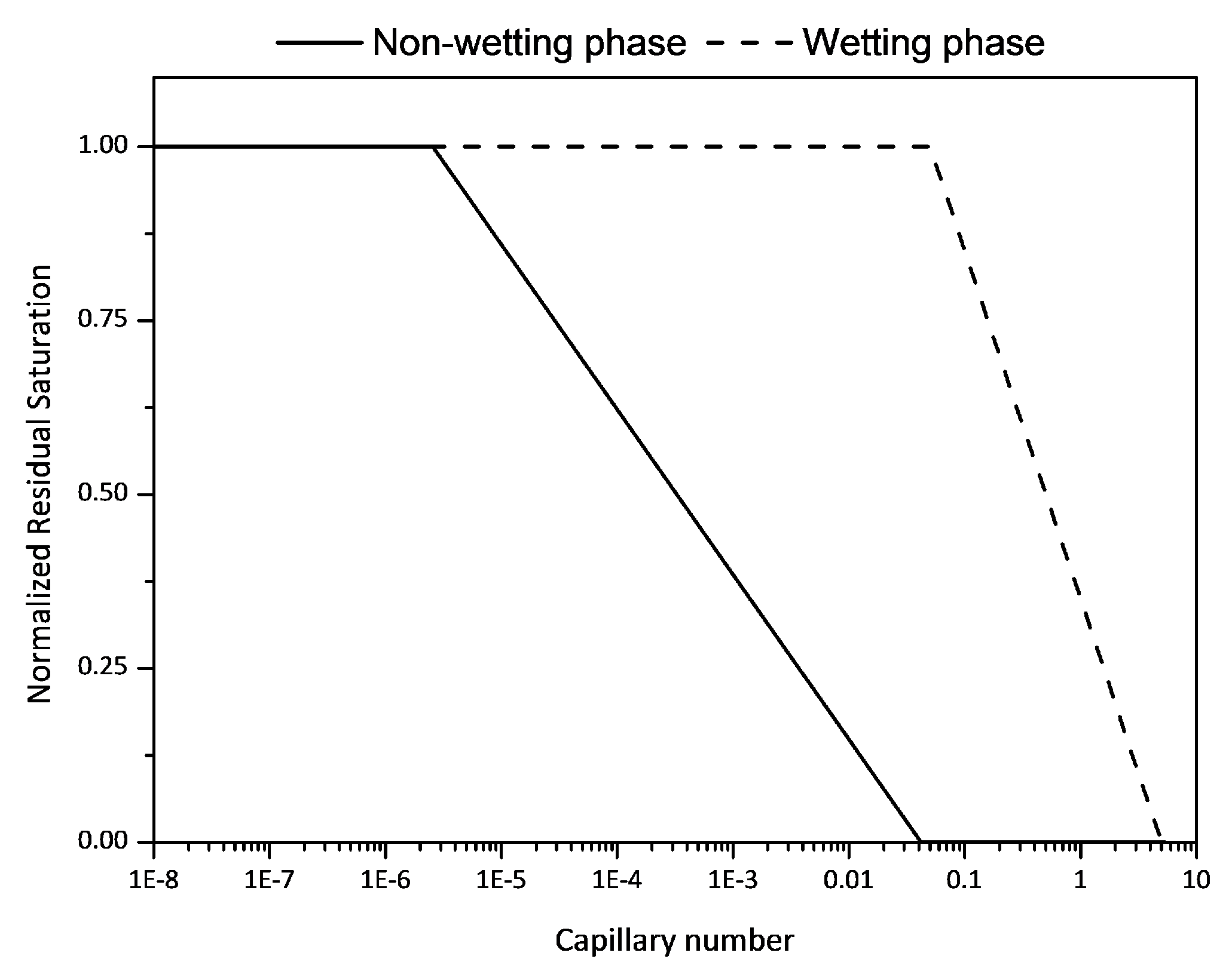
2.3.3. Residual Saturation
2.3.4. Relative Permeabilities
2.3.5. Phase Viscosities
3. Results and Discussion
3.1. Introduction
Data
3.2. Three-Component System
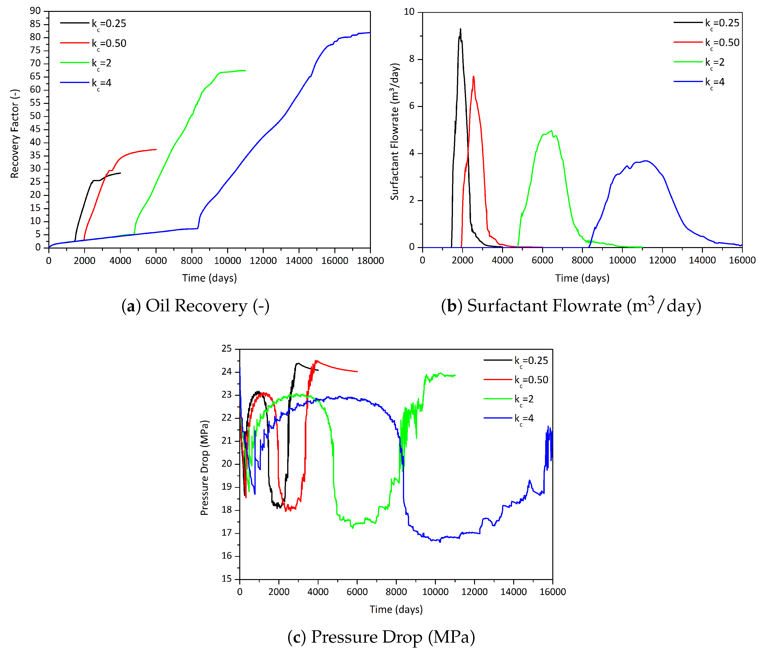
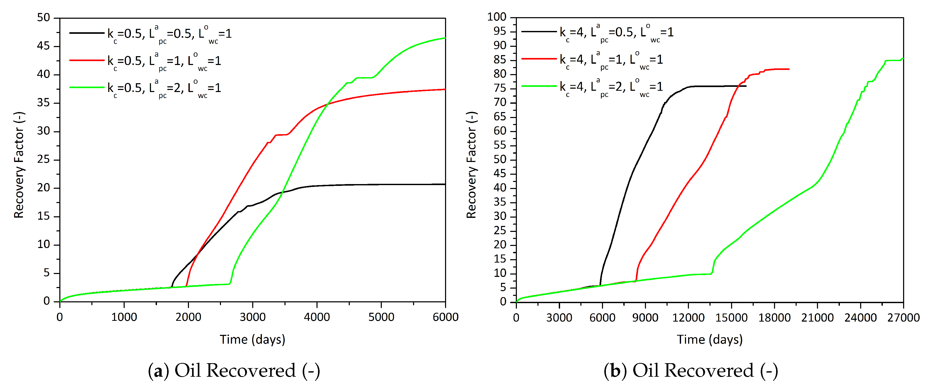
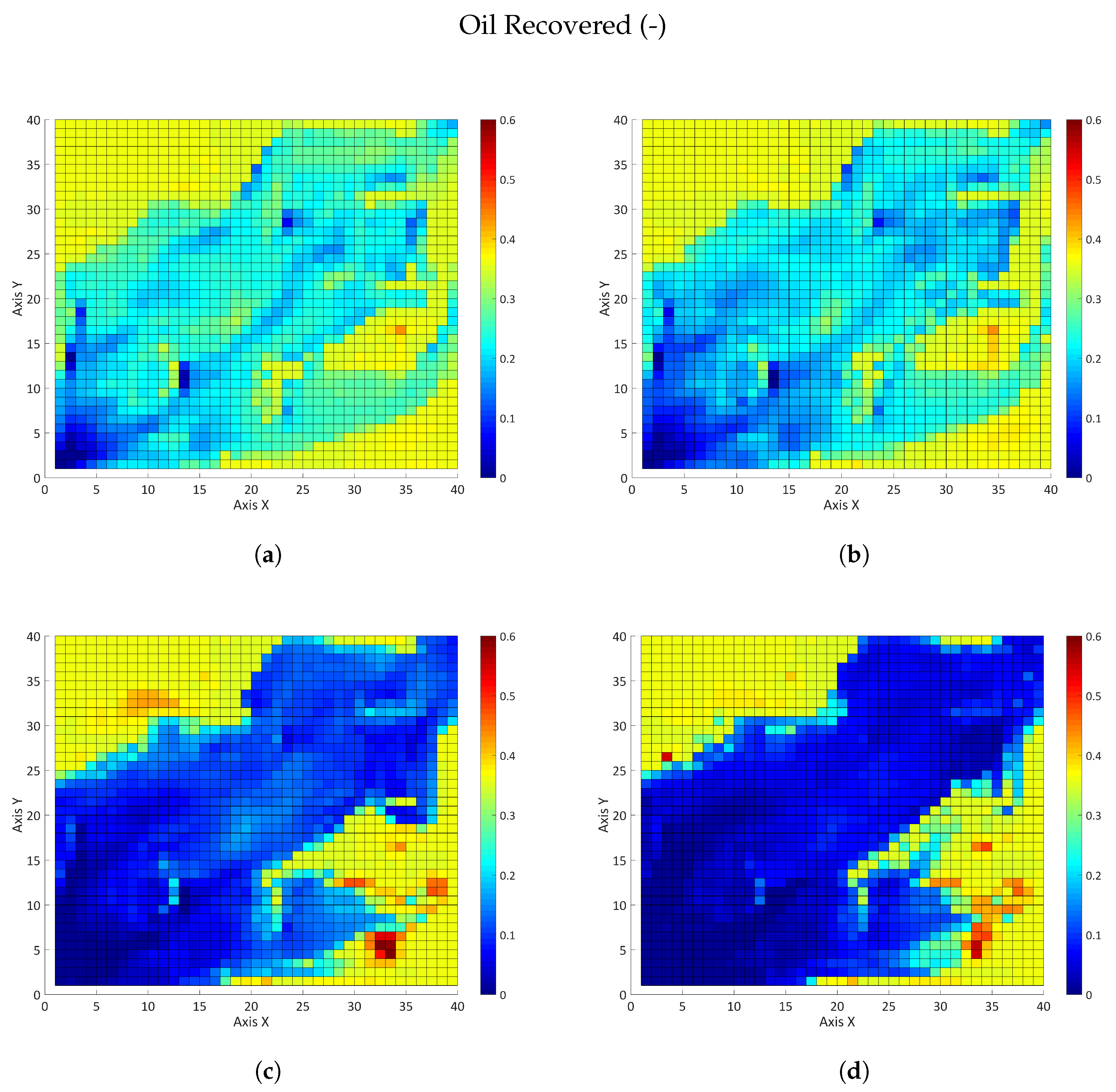
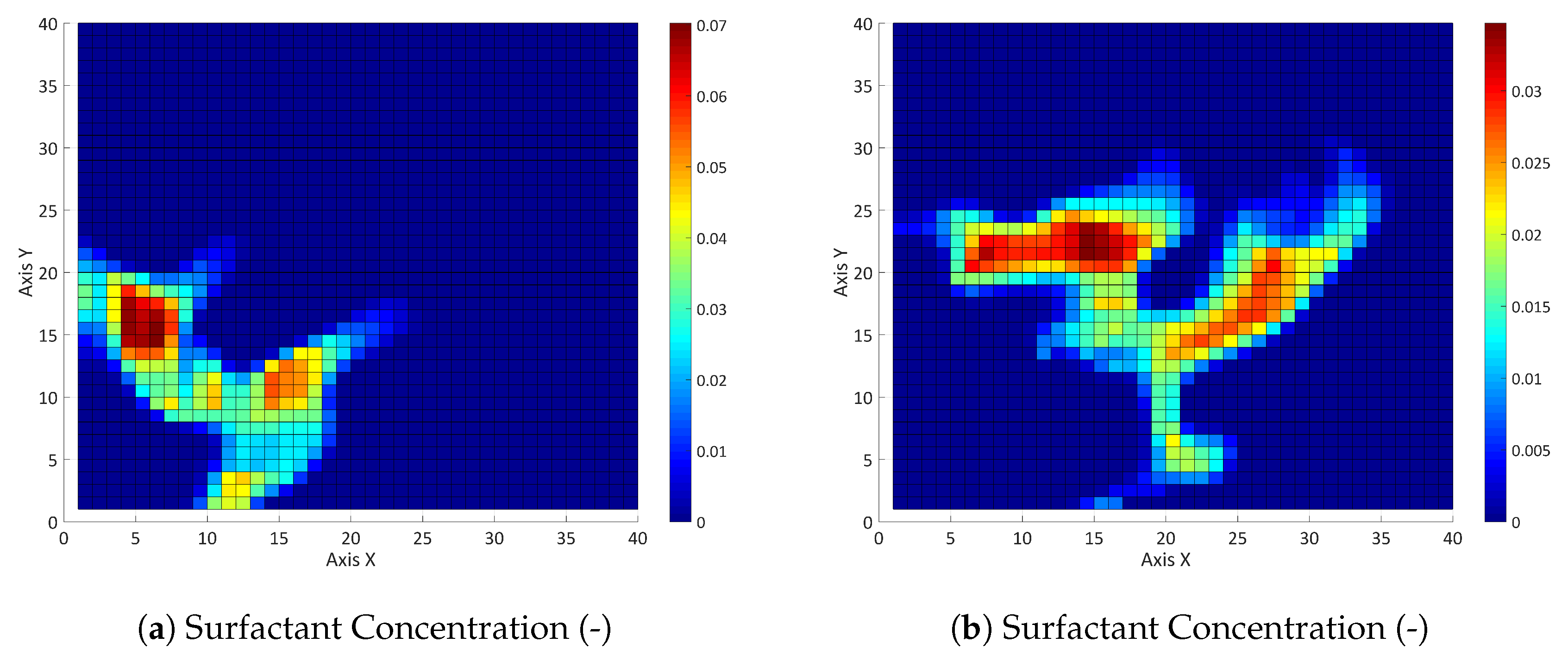
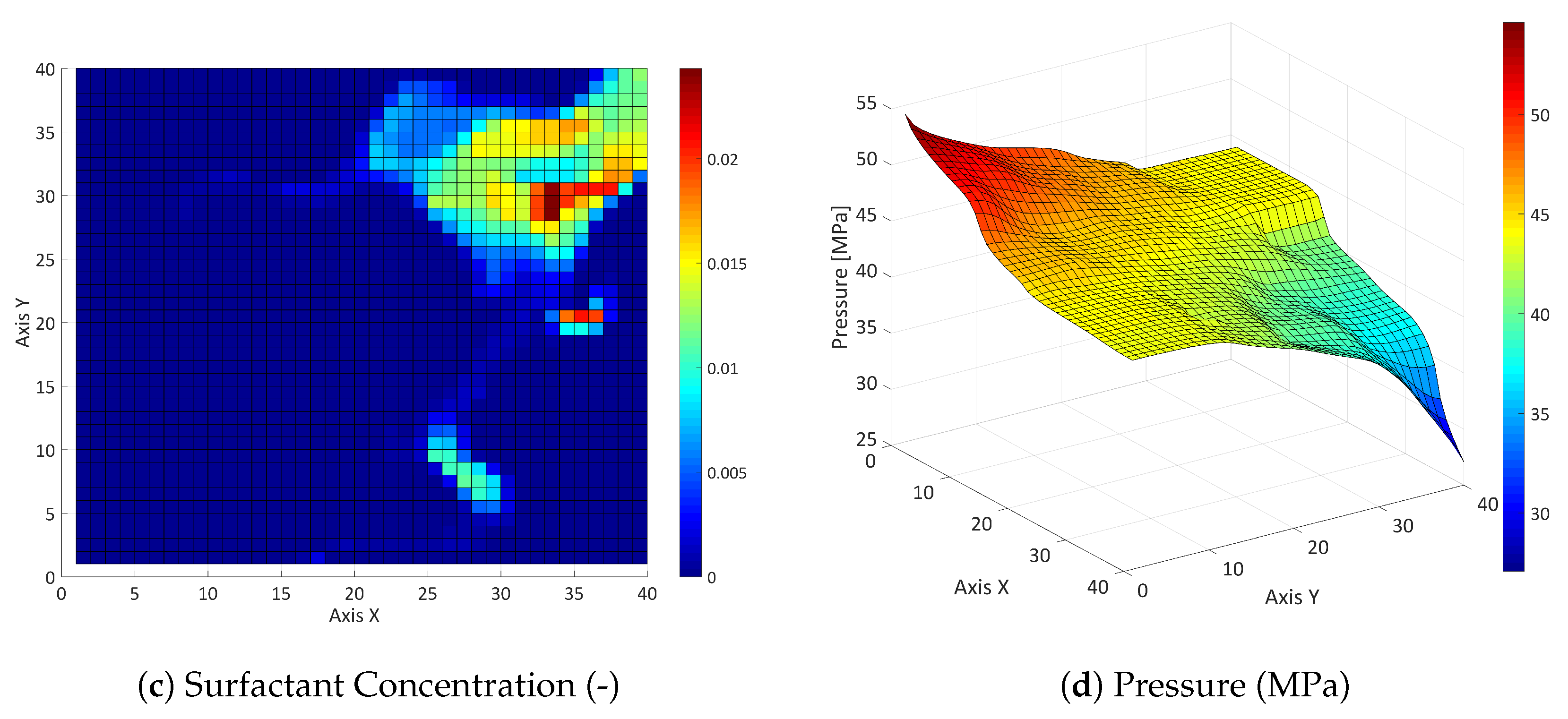
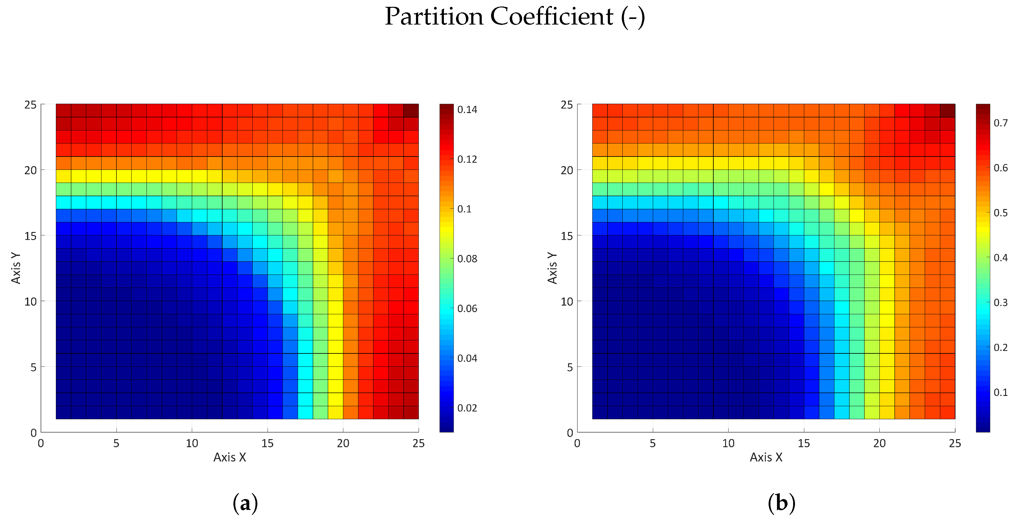
3.2.1. Influence of the Component Partitioning Parameters
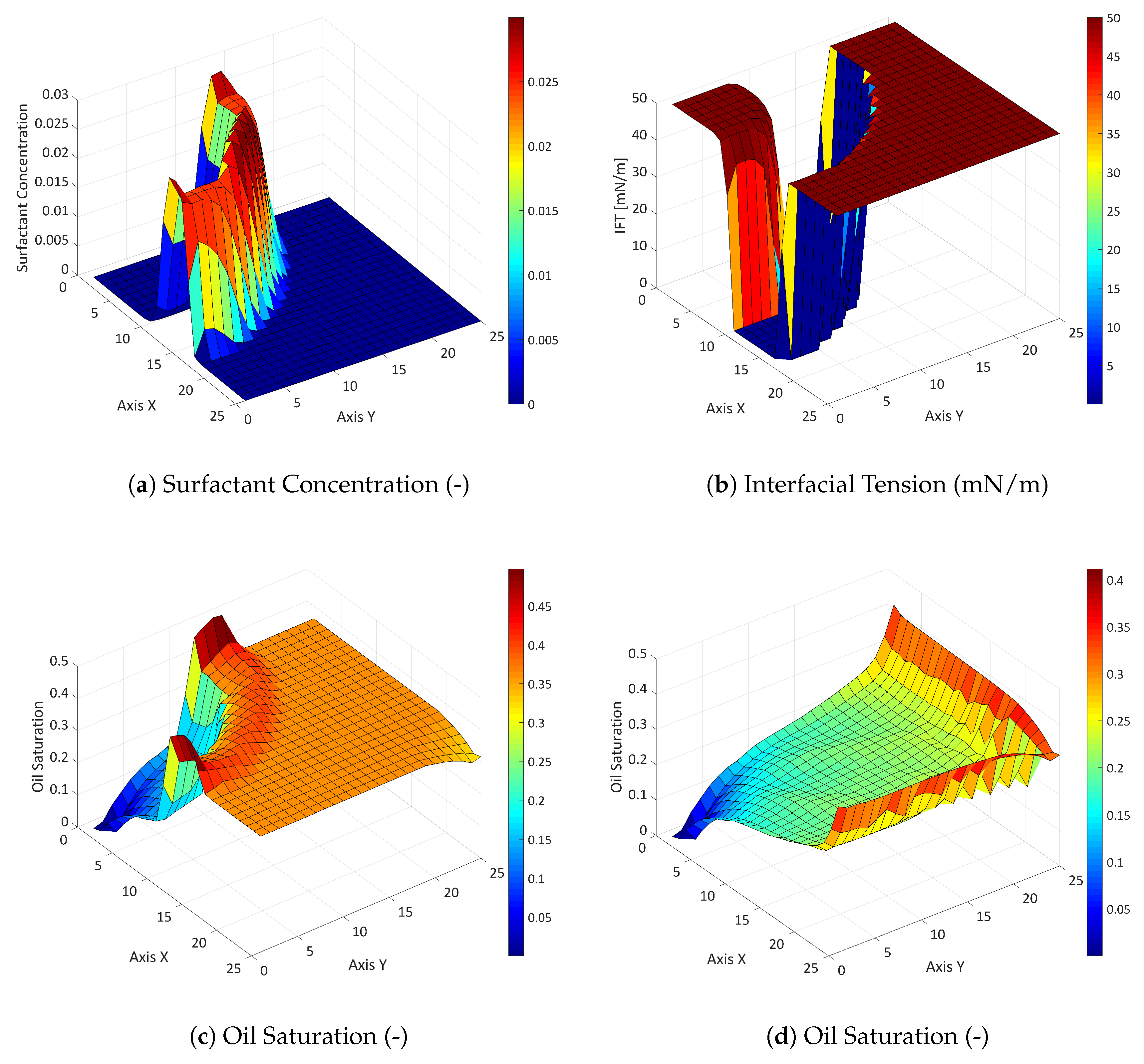
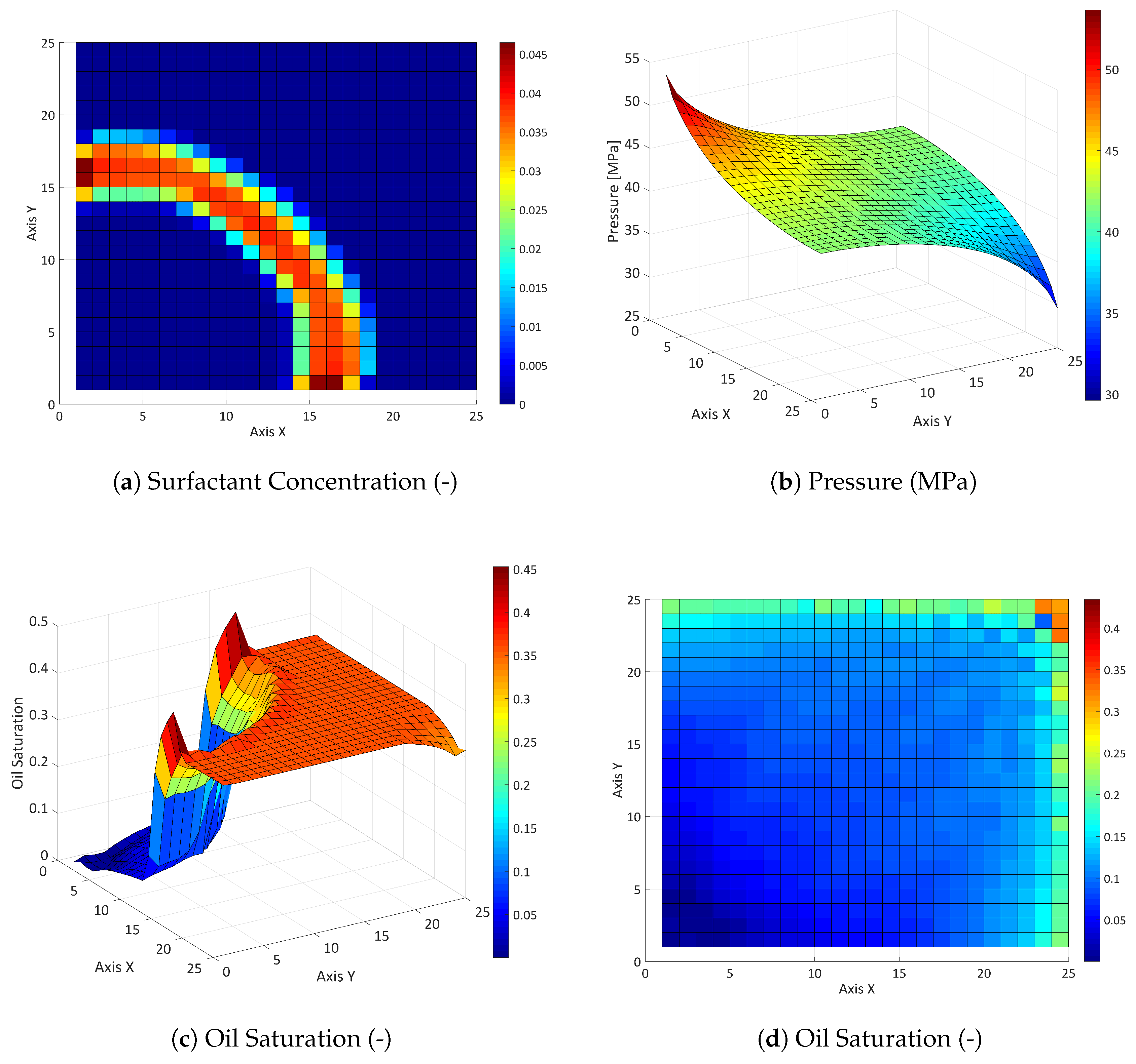
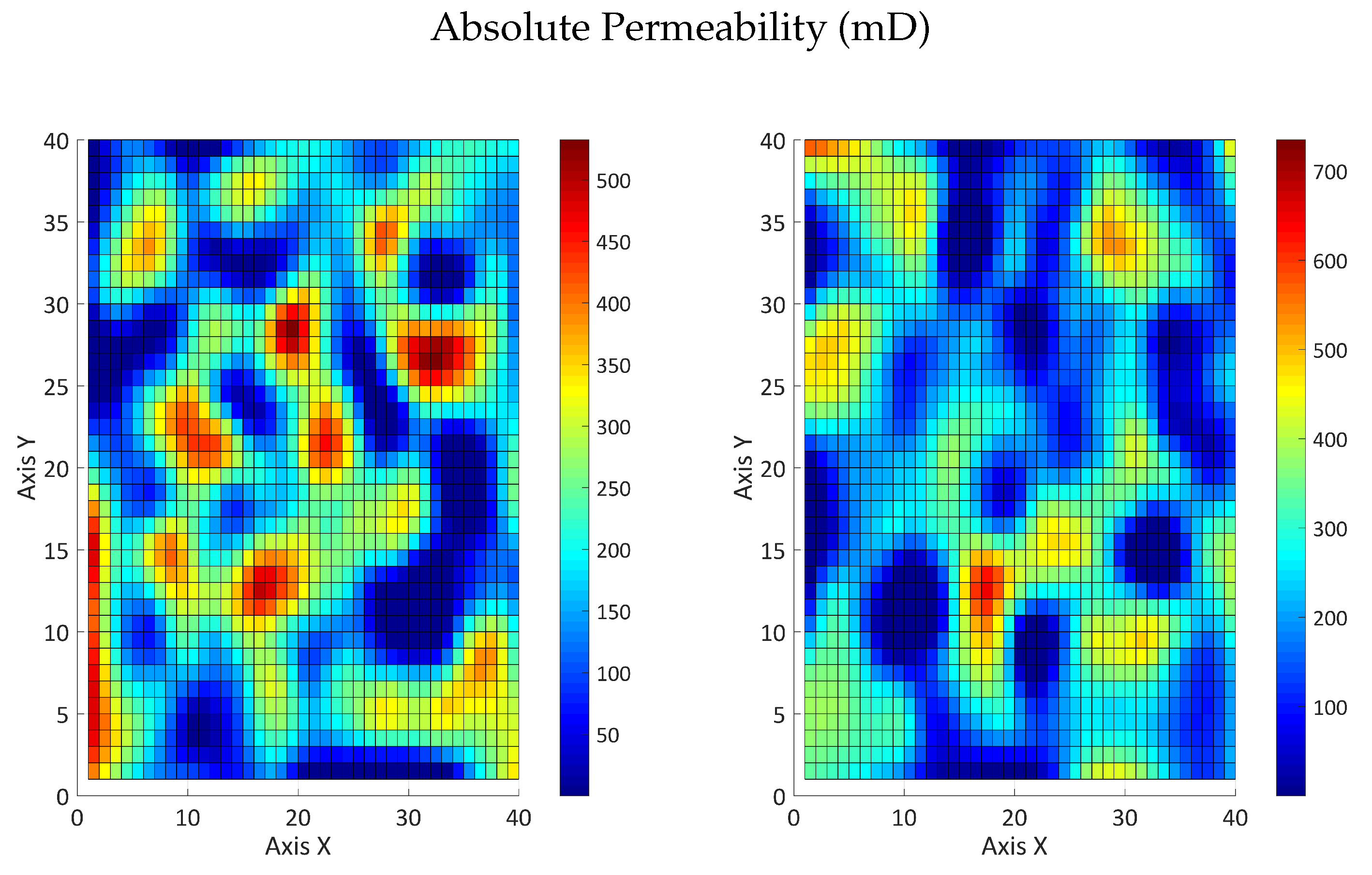
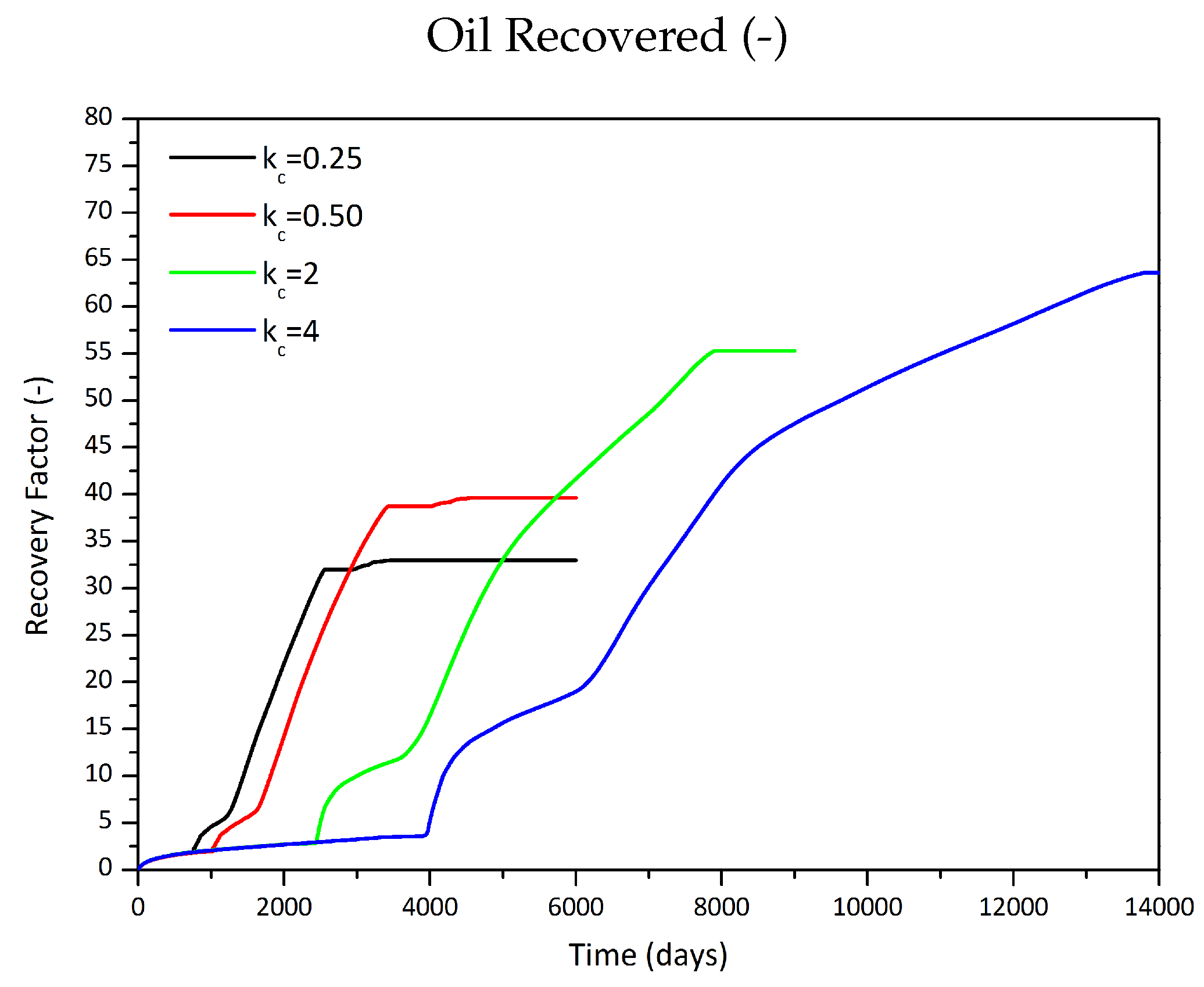
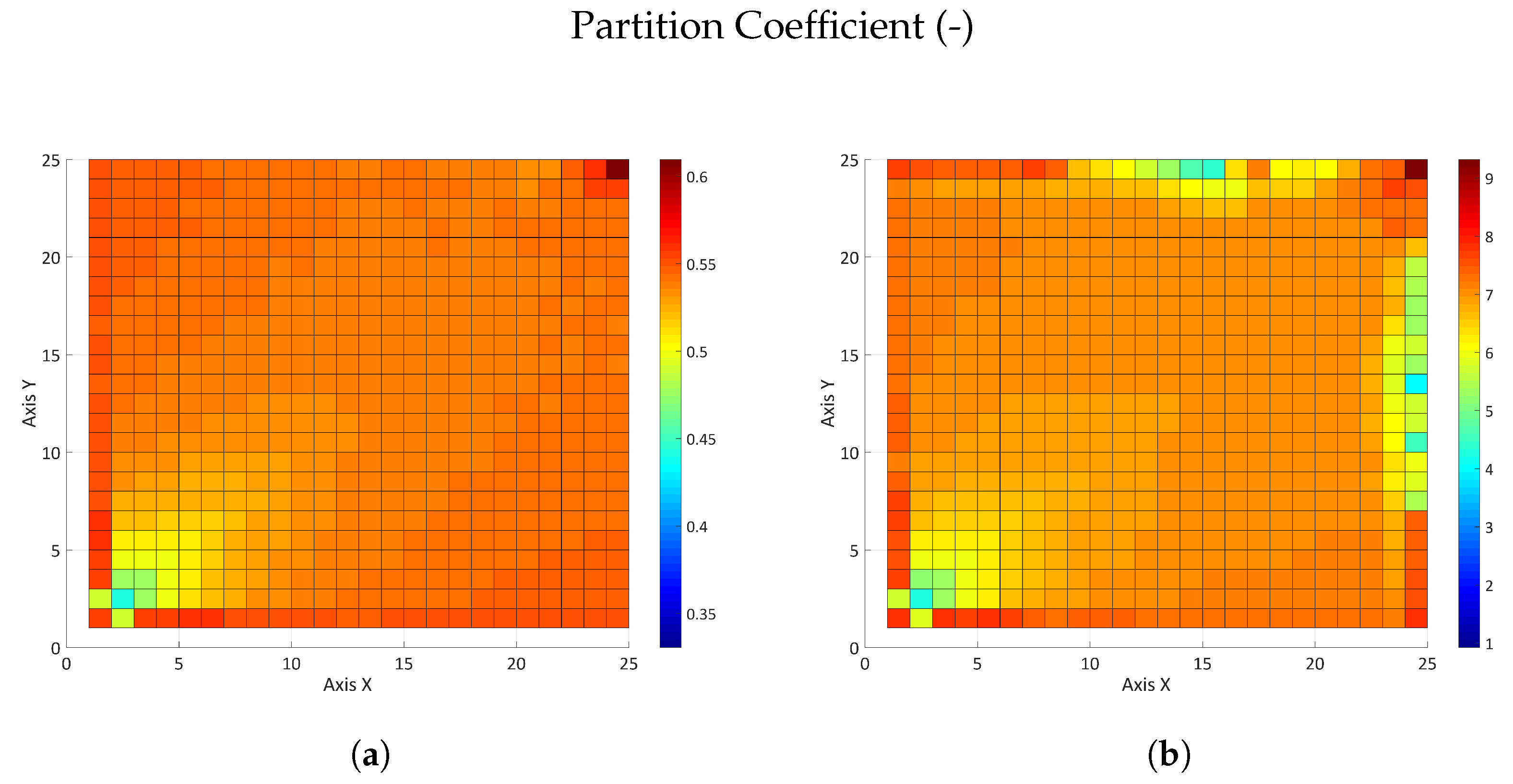
3.2.2. Influence of the Partition Coefficient in Random Permeability Fields
3.3. Four-Component System
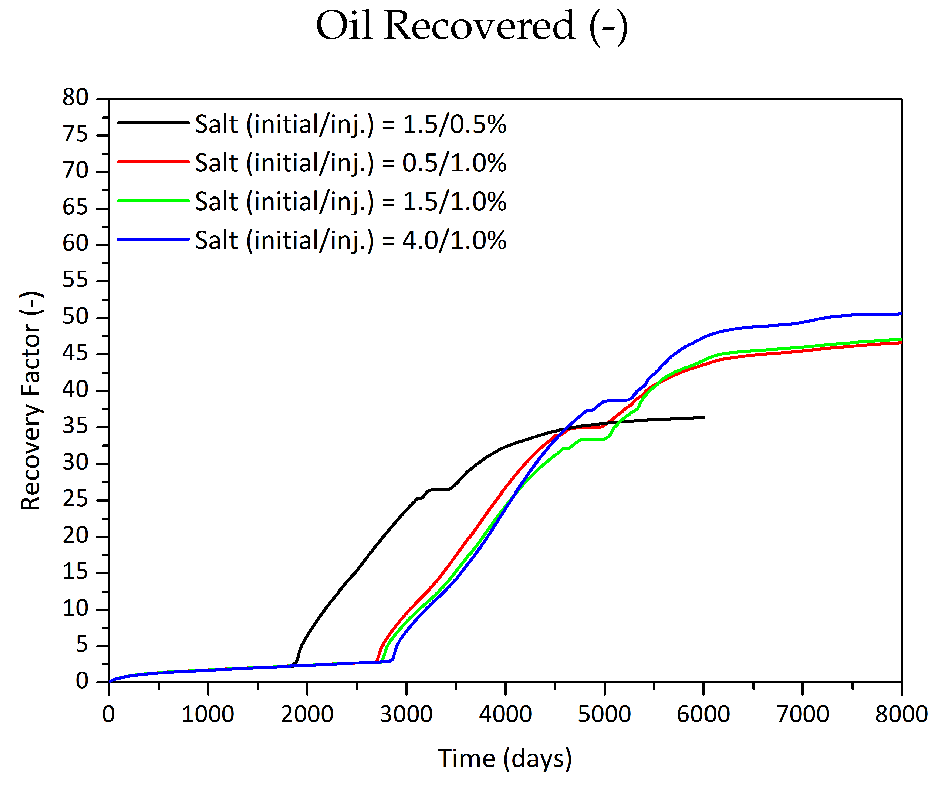
Influence of the Salt Component on the Phase Behaviour
4. Conclusions
Author Contributions
Funding
Acknowledgments
Conflicts of Interest
Abbreviations
| cEOR | Chemical Enhanced Oil Recovery |
| EOR | Enhanced Oil Recovery |
| IMPEC | Implicit Pressure, Explicit Concentration |
| OOIP | Original Oil in Place |
| IFT | Interfacial Tension |
| TDS | Total Dissolved Solids |
| TVD | Total Variation Diminishing |
| PDE | Partial Differential Equation |
| REV | Representative Elementary Volume |
| DPR | Disproportionate Permeability Reduction |
| CMC | Critical Micelle Concentration |
Nomenclature
| Component Adsorption [day–1] | Absolute Viscosity [Pa·s] | ||
| Rock Compressibility [Pa–1] | Interfacial Tension [mN/m] | ||
| D | Dispersion Tensor | Formation Porosity | |
| Molecular Diffusion [m2/s] | Reservoir Domain | ||
| Longitudinal Dispersion [m2/s] | |||
| Transversal Dispersion [m2/s] | Superscripts | ||
| Flux Limiting Function | a | Aqueous Phase | |
| K | Absolute Permeability [mD] | c | Capillary |
| Relative Permeability | H | Water-Oil System (no Chemical) | |
| p | Reservoir Pressure [Pa] | j | Phase |
| Bottomhole Pressure [Pa] | Time-Step | ||
| q | Flowrate [m3/day] | o | Oleous Phase |
| Well Radius [m] | r | Residual | |
| S | Phase Saturation | ||
| s | Well Skin Factor | Subscripts | |
| u | Darcy Velocity [m/day] | c | Surfactant Component |
| V | Volumetric Concentration | i | Component |
| z | Overall Concentration | Injection | |
| Spatial Grid Blocks | |||
| Greek Letters | p | Petroleum Component | |
| Domain Boundary | s | Salt Component | |
| Kronecker Delta | t | Total | |
| Phase Mobility [m2/(Pa·s)] | w | Water Component | |
References
- Owen, N.A.; Inderwildi, O.R.; King, D.A. The status of conventional world oil reserves-Hype or cause for concern? Energy Policy 2010, 38, 4743–4749. [Google Scholar] [CrossRef]
- BP. Statistical Review of World Energy; Annual Report 63; BP p.l.c.: London, UK, 2014. [Google Scholar]
- Dake, L.P. Fundamentals of Reservoir Engineering; Elsevier: Amsterdam, The Netherlands, 1978; ISBN 0-444-41830-X. [Google Scholar]
- Bidner, M.S. Propiedades de la Roca y los Fluidos en Reservorios de Petroleo; EUDEBA: Buenos Aires, Argentina, 2001; ISBN 9-502-31150-7. [Google Scholar]
- Satter, A.; Iqbal, G.M.; Buchwalter, J.L. Practical Enhanced Reservoir Engineering; PennWell Books: Tulsa, OK, USA, 2008; ISBN 978-1-59370-056-0. [Google Scholar]
- Schmidt, R.L.; Venuto, P.B.; Lake, L.W. A Niche for Enhanced Oil Recovery in the 1990’s. Oilfield Rev. 1992, 4, 55–61. [Google Scholar]
- Hirasaki, G.J.; Miller, C.A.; Puerto, M. Recent Advances in Surfactant EOR. SPE J. 2011, 16, 889–907. [Google Scholar] [CrossRef]
- Lake, L.W. Enhanced Oil Recovery; Prentice-Hall Inc.: Englewood Cliffs, NJ, USA, 1989; ISBN 0-13-281601-6. [Google Scholar]
- Druetta, P.; Yue, J.; Tesi, P.; Persis, C.D.; Picchioni, F. Numerical modeling of a compositional flow for chemical EOR and its stability analysis. Appl. Math. Model. 2017, 47, 141–159. [Google Scholar] [CrossRef]
- Druetta, P.; Tesi, P.; Persis, C.D.; Picchioni, F. Methods in Oil Recovery Processes and Reservoir Simulation. Adv. Chem. Eng. Sci. 2016, 6, 39. [Google Scholar] [CrossRef]
- Druetta, P.; Picchioni, F. Numerical Modeling and Validation of a Novel 2D Compositional Flooding Simulator Using a Second-Order TVD Scheme. Energies 2018, 11, 2280. [Google Scholar] [CrossRef]
- Garrett, H.E. Surface Active Chemicals; Pergamon Press: New York, NY, USA, 1972; ISBN 0-080-16422-6. [Google Scholar]
- Farrell, H.H.; Gregory, M.D.; Borah, M.T. Progress Report: Big Muddy Field Low-Tension Flood Demonstration Project With Emphasis on Injectivity and Mobility. In Proceedings of the SPE Enhanced Oil Recovery Symposium, Tulsa, OK, USA, 15–18 April 1984. [Google Scholar] [CrossRef]
- Reppert, T.R.; Bragg, J.R.; Wilkinson, J.R.; Snow, T.M.; Maer, N.K., Jr.; Gale, W.W. Second Ripley Surfactant Flood Pilot Test. In Proceedings of the SPE/DOE Enhanced Oil Recovery Symposium, Tulsa, OK, USA, 22–25 April 1990. [Google Scholar] [CrossRef]
- Maerker, J.M.; Gale, W.W. Surfactant flood process design for Loudon. SPE Reserv. Eng. 1992, 7, 36–44. [Google Scholar] [CrossRef]
- Green, D.W.; Willhite, G.P. Enhanced Oil Recovery; Society of Petroleum Engineers: Richardson, TX, USA, 1998; ISBN 978-1-55563-077-5. [Google Scholar]
- Iglauer, S.; Wu, Y.; Shuler, P.; Tang, Y.; Goddard, W.A., III. New surfactant classes for enhanced oil recovery and their tertiary oil recovery potential. J. Petrol. Sci. Engi. 2010, 71, 23–29. [Google Scholar] [CrossRef]
- Sheng, J.J. Status of surfactant EOR technology. Petroleum 2015, 1, 97–105. [Google Scholar] [CrossRef]
- Larson, R.G.; Davis, H.T.; Scriven, L.E. Elementary Mechanisms of Oil-Recovery by Chemical Methods. J. Petrol. Technol. 1982, 34, 243–258. [Google Scholar] [CrossRef]
- Pashley, R.M.; Karaman, M.E. Surfactants and Self-Assembly; Applied Colloid and Surface Chemistry; John Wiley & Sons, Ltd.: Chichester, UK, 2004; pp. 61–77. ISBN 978-0-47001-470-7. [Google Scholar] [CrossRef]
- Adibhatla, B.; Mohanty, K.K. Parametric analysis of surfactant-aided imbibition in fractured carbonates. J. Colloid Interface Sci. 2008, 317, 513–522. [Google Scholar] [CrossRef]
- Akin, S.; Kovscek, A.R. Computed tomography in petroleum engineering research. Geol. Soc. Lond. Spec. Publ. 2003, 215, 23–38. [Google Scholar] [CrossRef]
- Yu, Q.; Jiang, H.; Zhao, C. Study of Interfacial Tension Between Oil and Surfactant Polymer Flooding. Petrol. Sci. Technol. 2010, 28, 1846–1854. [Google Scholar] [CrossRef]
- Kou, J.; Sun, S.; Wang, X. Linearly Decoupled Energy-Stable Numerical Methods for Multicomponent Two-Phase Compressible Flow. SIAM J. Numer. Anal. 2018, 56, 3219–3248. [Google Scholar] [CrossRef]
- El-Amin, M.; Kou, J.; Sun, S.; Salama, A. Adaptive Time-Splitting Scheme for Two-Phase Flow in Heterogeneous Porous Media. Adv. Geo-Energy Res. 2017, 1, 182–189. [Google Scholar] [CrossRef]
- Lake, L.; Pope, G.; Carey, G.; Sepehrnoori, K. Isothermal, Multiphase, Multicomponent Fluid-Flow in Permeable Media. 1. Description and Mathematical Formulation. In Situ 1984, 8, 1–40. [Google Scholar]
- Pope, G.A.; Carey, G.F.; Sepehrnoori, K. Isothermal, Multiphase, Multicomponent Fluid-Flow in Permeable Media. 2. Numerical Techniques and Solution. In Situ 1984, 8, 41–97. [Google Scholar]
- Helfferich, F. Theory of Multicomponent, Multiphase Displacement in Porous-Media. Soc. Petrol. Eng. J. 1981, 21, 51–62. [Google Scholar] [CrossRef]
- Fleming, P.; Thomas, C.; Winter, W. Formulation of a General Multiphase, Multicomponent Chemical Flood Model. Soc. Petrol. Eng. J. 1981, 21, 63–76. [Google Scholar] [CrossRef]
- Thomas, C.; Fleming, P.; Winter, W. A Ternary, 2-Phase, Mathematical-Model of Oil-Recovery with Surfactant Systems. Soc. Petrol. Eng. J. 1984, 24, 606–616. [Google Scholar] [CrossRef]
- Larson, R.G. Analysis of the Physical Mechanisms in Surfactant Flooding. Soc. Petrol. Eng. J. 1978, 18, 42–58. [Google Scholar] [CrossRef]
- Hirasaki, G.J. Application of the Theory of Multicomponent, Multiphase Displacement to 3-Component, 2-Phase Surfactant Flooding. Soc. Petrol. Eng. J. 1981, 21, 191–204. [Google Scholar] [CrossRef]
- Larson, R.G. The Influence of Phase Behavior on Surfactant Flooding. Soc. Petrol. Eng. J. 1979, 19, 411–422. [Google Scholar] [CrossRef]
- Morshedi, S.; Foroughi, S.; Beiranvand, M.S. Numerical Simulation of Surfactant Flooding in Darcy Scale Flow. Petrol. Sci. Technol. 2014, 32, 1365–1374. [Google Scholar] [CrossRef]
- Yin, D.-Y.; Pu, H. Numerical Simulation Study on Surfactant Flooding for Low Permeability Oilfield in the Condition of Threshold Pressure. J. Hydrodyn. 2008, 20, 492–498. [Google Scholar] [CrossRef]
- Yin, D.; Zhou, Y. Numerical Simulation of Surfactant Flooding and Its Application in Low Permeability Reservoir. Int. J. Control Autom. 2013, 6, 451–472. [Google Scholar]
- Porcelli, P.; Bidner, M. Simulation and Transport Phenomena of a Ternary 2-Phase Flow. Transp. Porous Media 1994, 14, 101–122. [Google Scholar] [CrossRef]
- Bidner, M.S.; Savioli, G.B. On the Numerical Modeling for Surfactant Flooding of Oil Reservoirs. Mec. Comput. 2002, XXI, 566–585. [Google Scholar]
- Rai, S.; Bera, A.; Mandal, A. Modeling of surfactant and surfactant-polymer flooding for enhanced oil recovery using STARS (CMG) software. J. Petrol. Explor. Prod. Technol. 2015, 5, 1–11. [Google Scholar] [CrossRef]
- Sulaiman, W.; Lee, E.S. Simulation of surfactant based enhanced oil recovery. J. Petrol. Gas Eng. 2012, 3, 58–73. [Google Scholar]
- Camilleri, D.; Engelson, S.; Lake, L.W.; Lin, E.C.; Ohnos, T.; Pope, G.; Sepehrnoori, K. Description of an Improved Compositional Micellar/Polymer Simulator. SPE Reserv. Eng. 1987, 2, 427–432. [Google Scholar] [CrossRef]
- Camilleri, D.; Fil, A.; Pope, G.A.; Rouse, B.A.; Sepehrnoori, K. Comparison of an Improved Compositional Micellar/Polymer Simulator With Laboratory Corefloods. SPE Reserv. Eng. 1987, 2, 441–451. [Google Scholar] [CrossRef]
- Delshad, M.; Najafabadi, N.F.; Anderson, G.; Pope, G.A.; Sepehrnoori, K. Modeling Wettability Alteration By Surfactants in Naturally Fractured Reservoirs. SPE Reserv. Eval. Eng. 2009, 12, 361–370. [Google Scholar] [CrossRef]
- Patacchini, L.; de Loubens, R.; Moncorge, A.; Trouillaud, A. Four-Fluid-Phase, Fully Implicit Simulation of Surfactant Flooding. SPE Reserv. Eval. Eng. 2014, 17, 271–285. [Google Scholar] [CrossRef]
- Hand, D.B. Dineric Distribution. J. Phys. Chem. 1929, 34, 1961–2000. [Google Scholar] [CrossRef]
- Prouvost, L.; Pope, G.; Rouse, B. Microemulsion Phase-Behavior—A Thermodynamic Modeling of the Phase Partitioning of Amphiphilic Species. Soc. Petrol. Eng. J. 1985, 25, 693–703. [Google Scholar] [CrossRef]
- Prouvost, L.P.; Satoh, T.; Sepehrnoori, K.; Pope, G.A. A New Micellar Phase-Behavior Model for Simulating Systems with Up to Three Amphiphilic Species. In Proceedings of the SPE Annual Technical Conference and Exhibition, Houston, TX, USA, 16–19 September 1984. [Google Scholar] [CrossRef]
- Saad, N.; Pope, G.A.; Sepehrnoorl, K. Application of higher-order methods in compositional simulation. SPE Reserv. Eng. 1990, 5, 623–630. [Google Scholar] [CrossRef]
- Delshad, M.; Pope, G.; Sepehrnoori, K. UTCHEM Version 9.0 Technical Documentation; Center for Petroleum and Geosystems Engineering, The University of Texas at Austin: Austin, TX, USA, 2000; Volume 78751. [Google Scholar]
- Yuan, C. Commercial Scale Simulations of Surfactant/Polymer Flooding. Ph.D. Thesis, The University of Texas at Austin, Austin, TX, USA, 2012. [Google Scholar]
- Sheng, J. Modern Chemical Enhanced Oil Recovery; Elsevier: Amsterdam, The Netherlands, 2011; ISBN 978-0-08096-163-7. [Google Scholar]
- Bidner, M.; Porcelli, P. Influence of phase behavior on chemical flood transport phenomena. Transp. Porous Media 1996, 24, 247–273. [Google Scholar] [CrossRef]
- Bidner, M.; Porcelli, P. Influence of capillary pressure, adsorption and dispersion on chemical flood transport phenomena. Transp. Porous Media 1996, 24, 275–296. [Google Scholar] [CrossRef]
- Bear, J. Dynamics of Fluids In Porous Media; American Elsevier Publishing Company: New York, NY, USA, 1972; ISBN 978-0-44400-114-6. [Google Scholar]
- Chen, Z.; Huan, G.; Ma, Y. Computational Methods for Multiphase Flows in Porous Media; Society for Industrial and Applied Mathematics: Philadelphia, PA, USA, 2006; ISBN 978-0-89871-606-1. [Google Scholar] [CrossRef]
- Kuzmin, D. A Guide to Numerical Methods for Transport Equations; University Erlangen-Nuremberg: Erlangen, Germany, 2010. [Google Scholar]
- Liu, J.; Delshad, M.; Pope, G.A.; Sepehrnoori, K. Application of higher-order flux-limited methods in compositional simulation. Transp. Porous Media 1994, 16, 1–29. [Google Scholar] [CrossRef]
- Barrett, R.; Berry, M.; Chan, T.; Demmel, J.; Donato, J.; Dongarra, J.; Eijkhout, V.; Pozo, R.; Romine, C.; Van der Vorst, H. Templates for the Solution of Linear Systems: Building Blocks for Iterative Methods; Society for Industrial and Applied Mathematics: Philadelphia, PA, USA, 1994; ISBN 978-0-89871-328-2. [Google Scholar] [CrossRef]
- Kamalyar, K.; Kharrat, R.; Nikbakht, M. Numerical Aspects of the Convection-Dispersion Equation. Petrol. Sci. Technol. 2014, 32, 1729–1762. [Google Scholar] [CrossRef]
- Attwood, D.; Florence, A.T. Surfactant Systems—Their Chemistry, Pharmacy and Biology; Chapman and Hall: London, UK, 1983; ISBN 978-9-40095-775-6. [Google Scholar]
- El-Dessouky, H.; Ettouney, H.M. Fundamentals of Salt Water Desalination; Elsevier Science: Amsterdam, The Netherlands, 2002; ISBN 978-0-08053-212-7. [Google Scholar]
- Ghannam, M.T.; Hasan, S.W.; Abu-Jdayil, B.; Esmail, N. Rheological properties of heavy & light crude oil mixtures for improving flowability. J. Petrol. Sci. Eng. 2012, 81, 122–128. [Google Scholar] [CrossRef]
- Bhuyan, D.; Lake, L.W.; Pope, G.A. Mathematical Modeling of High-pH Chemical Flooding. SPE Reserv. Eng. 1990, 5, 213–220. [Google Scholar] [CrossRef]
- Delshad, M.; Han, C.; Sepehrnoori, K.; Najafabadi, N.F. Development of a Three Phase, Fully Implicit, Parallel Chemical Flood Simulator. In Proceedings of the SPE Reservoir Simulation Symposium, The Woodlands, TX, USA, 2–4 February 2009. [Google Scholar] [CrossRef]
- Han, C.; Delshad, M.; Pope, G.A.; Sepehrnoori, K. Coupling EOS Compositional and Surfactant Models in a Fully Implicit Parallel Reservoir Simulator Using EACN Concept. In Proceedings of the SPE Annual Technical Conference and Exhibition, San Antonio, TX, USA, 24–27 September 2006. [Google Scholar] [CrossRef]
- Lotfollahi, M.; Varavei, A.; Delshad, M.; Farajzadeh, R.; Pope, G.A. A Four-Phase Flow Model to Simulate Chemical EOR with Gas. In Proceedings of the SPE Reservoir Simulation Symposium, Houston, TX, USA, 23–25 February 2015. [Google Scholar] [CrossRef]
- Nelson, R.C.; Pope, G.A. Phase Relationships in Chemical Flooding. Soc. Petrol. Eng. J. 1978, 18, 325–338. [Google Scholar] [CrossRef]
- Pope, G.A.; Nelson, R.C. A Chemical Flooding Compositional Simulator. Soc. Petrol. Eng. J. 1978, 18, 339–354. [Google Scholar] [CrossRef]
- Aulia, A.; El-Khatib, N.A. Mathematical Description of the Implementation of the Adaptive Newton-Raphson Method in Compositional Porous Media Flow. Int. J. Basic Appl. Sci. 2010, 10, 108–115. [Google Scholar]
- Fadili, A.; Kristensen, M.R.; Moreno, J. Smart Integrated Chemical EOR Simulation. In Proceedings of the International Petroleum Technology Conference, Doha, Qatar, 7–9 December 2009. [Google Scholar] [CrossRef]
- Liu, S.; Miller, C.A.; Li, R.F.; Hirasaki, G. Alkaline/Surfactant/Polymer Processes: Wide Range of Conditions for Good Recovery. SPE J. 2010, 15, 282–293. [Google Scholar] [CrossRef]


| Geometrical Data of the Reservoir | |||||
| Length in axis X | 500 m | Length in axis Y | 500 m | Layer thickness | 5 m |
| elements | 25/40 | elements | 25/40 | ||
| Rock Properties | |||||
| Porosity | 0.25 | 200 mD | 200 mD | ||
| Initial Conditions | |||||
| 0.36 | (EOR) | 0.35 | 0.15 | ||
| Simulation Data | |||||
| Total time | 6000 days | Chem. injection period | 200 days | 0.025 | |
| Phases’ Physical Data | |||||
| 1 cP | 5 cP | Oil density | 850 kg/m | ||
| Water density | 1020 kg/m | IFT | 50 mN/m | ||
| Physical Data | |||||
| Number of wells | 2 | Well radius | 0.25 m | Skin factor | 0 |
| Operating Conditions | |||||
| Total production flowrate | 1650 STB/day | Bottomhole pressure | 55,160 kPa | ||
| Partition Coefficient | Solubilization/Swelling | Oil Recovered | |
|---|---|---|---|
| - | - | m | %OOIP |
| 0.25 | 1 | 32,068 | 28.5 |
| 0.5 | 1 | 42,160 | 37.5 |
| 2 | 1 | 75,931 | 67.5 |
| 4 | 1 | 92,181 | 81.9 |
| Oil Recovered | Oil Recovered | ||||||||
|---|---|---|---|---|---|---|---|---|---|
| - | - | - | m | %OOIP | - | - | - | m | %OOIP |
| 0.25 | 0.5 | 1 | 19,125 | 17.0 | 2 | 0.5 | 1 | 66,183 | 58.8 |
| 0.25 | 1 | 0.5 | 31,752 | 28.2 | 2 | 1 | 0.5 | 40,379 | 35.9 |
| 0.25 | 1 | 1 | 32,068 | 28.5 | 2 | 1 | 1 | 75,931 | 67.5 |
| 0.25 | 2 | 1 | 37,572 | 33.4 | 2 | 2 | 1 | 83,092 | 73.9 |
| 0.25 | 1 | 2 | 32,348 | 28.8 | 2 | 1 | 2 | 76,700 | 68.2 |
| 0.5 | 0.5 | 1 | 23,322 | 20.7 | 4 | 0.5 | 1 | 85,488 | 76.0 |
| 0.5 | 1 | 0.5 | 41,961 | 37.3 | 4 | 1 | 0.5 | 45,641 | 40.6 |
| 0.5 | 1 | 1 | 42,160 | 37.5 | 4 | 1 | 1 | 92,181 | 81.9 |
| 0.5 | 2 | 1 | 52,385 | 46.6 | 4 | 2 | 1 | 96,478 | 85.8 |
| 0.5 | 1 | 2 | 42,629 | 37.9 | 4 | 1 | 2 | 92,822 | 82.5 |
| Partition Coefficient | Solubilization/Swelling | Oil Recovered | |
|---|---|---|---|
| - | - | m | %OOIP |
| 0.25 | 1 | 37,075 | 33.0 |
| 0.5 | 1 | 44,605 | 39.7 |
| 2 | 1 | 62,246 | 55.3 |
| 4 | 1 | 71,596 | 63.6 |
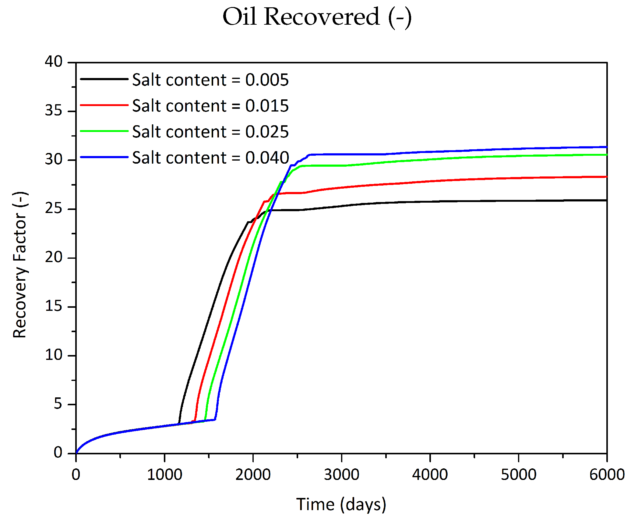
| Initial Salt Content | Critical Salt Content | Oil Recovered | |
|---|---|---|---|
| % | % | m | %OOIP |
| 0.5 | 2 | 29,153 | 25.9 |
| 1.5 | 2 | 31,866 | 28.3 |
| 2.5 | 2 | 34,405 | 30.6 |
| 4 | 2 | 35,302 | 31.4 |
| Initial Salt Content | Critical Salt Content | Salt Injected | Oil Recovered | |
|---|---|---|---|---|
| % | % | % | m | %OOIP |
| 0.5 | 2 | 1 | 52,460 | 46.6 |
| 1.5 | 2 | 0.5 | 40,926 | 36.4 |
| 1.5 | 2 | 1 | 52,997 | 47.1 |
| 1.5 | 2 | 1.5 | 80,758 | 71.8 |
| 4 | 2 | 1 | 57,152 | 50.8 |
© 2019 by the authors. Licensee MDPI, Basel, Switzerland. This article is an open access article distributed under the terms and conditions of the Creative Commons Attribution (CC BY) license (http://creativecommons.org/licenses/by/4.0/).
Share and Cite
Druetta, P.; Picchioni, F. Simulation of Surfactant Oil Recovery Processes and the Role of Phase Behaviour Parameters. Energies 2019, 12, 983. https://doi.org/10.3390/en12060983
Druetta P, Picchioni F. Simulation of Surfactant Oil Recovery Processes and the Role of Phase Behaviour Parameters. Energies. 2019; 12(6):983. https://doi.org/10.3390/en12060983
Chicago/Turabian StyleDruetta, Pablo, and Francesco Picchioni. 2019. "Simulation of Surfactant Oil Recovery Processes and the Role of Phase Behaviour Parameters" Energies 12, no. 6: 983. https://doi.org/10.3390/en12060983
APA StyleDruetta, P., & Picchioni, F. (2019). Simulation of Surfactant Oil Recovery Processes and the Role of Phase Behaviour Parameters. Energies, 12(6), 983. https://doi.org/10.3390/en12060983