Article

A Horizon Optimization Control Framework for the Coordinated Operation of Multiple Distributed Energy Resources in Low Voltage Distribution Networks

1
Efacec, Division of Smart Grids, 4471-907 Porto, Portugal
2
Efacec, Division of Storage, 4471-907 Porto, Portugal
3
Efacec, Division of T&I, 4466-952 Porto, Portugal
4
Faculty of Engineering (FEUP), University of Porto, 4200-465 Porto, Portugal
*
Author to whom correspondence should be addressed.
Current address: Via de Francisco Sá Carneiro Apartado 3078, 4471-907 Moreira da Maia, Porto, Portugal.
Energies 2019, 12(6), 1182; https://doi.org/10.3390/en12061182
Submission received: 27 February 2019 / Revised: 19 March 2019 / Accepted: 21 March 2019 / Published: 26 March 2019
(This article belongs to the Special Issue Distributed Energy Resources Management 2018)

Abstract

:
In recent years, the installation of residential Distributed Energy Resources (DER) that produce (mainly rooftop photovoltaics usually bundled with battery system) or consume (electric heat pumps, controllable loads, electric vehicles) electric power is continuously increasing in Low Voltage (LV) distribution networks. Several technical challenges may arise through the massive integration of DER, which have to be addressed by the distribution grid operator. However, DER can provide certain degree of flexibility to the operation of distribution grids, which is generally performed with temporal shifting of energy to be consumed or injected. This work advances a horizon optimization control framework which aims to efficiently schedule the LV network’s operation in day-ahead scale coordinating multiple DER. The main objectives of the proposed control is to ensure secure LV grid operation in the sense of admissible voltage bounds and rated loading conditions for the secondary transformer. The proposed methodology leans on a multi-period three-phase Optimal Power Flow (OPF) addressed as a nonlinear optimization problem. The resulting horizon control scheme is validated within an LV distribution network through multiple case scenarios with high microgeneration and electric vehicle integration providing admissible voltage limits and avoiding unnecessary active power curtailments.

1. Introduction

Nowadays, an increasing number of small-scale units, typically referred to Distributed Energy Resources (DER), is connected along the Low Voltage (LV) distribution networks posing several technical challenges, whilst bringing novel and diverse opportunities. Most commonly there is already a large share of injected power at the distribution level by the renewable energy merely based on solar energy through Photovoltaic (PV). The connection of such resources at the LV grid and end-users’ premises is foreseen to increase substantially in the close future with small rooftop installation usually coupled with Battery Storage System (BESS), controllable loads (e.g., Electric Water Heaters) and Electric Vehicles (EV). Therefore, it shall be critical to exploit the DER controllability and active participation through demand response schemes in order to support or even improve techno-economically the operation of the distribution networks operation [1,2]. For instance, DERs might be used to provide technical support to tackle voltage or congestion problems delivering profits to the end-consumers accordingly.
Traditionally, LV networks used to be the most passive circuits within the power systems, since power flows were solely headed from distribution transformers to consumers without the operation of automation elements [3]. In particular, the entire segment from the secondary substation and its downstream connected LV networks is very often not monitored nor controlled [4].
The Distribution System Operators (DSOs) address such technical challenges by increasing the observability and controllability of the grids, envisioning the active management of the DERs for ancillary services, throughout new operation stages [5,6]. Such attributes of advanced control and monitoring techniques do typically refer to Advanced Distribution Management Systems (A-DMS) [7]. The active management of distribution networks through the engagement of DERs in the operation of the grid is regarded to occur with the provision of flexibilities services such as active and reactive power control (i.e., inverter based control). The smart grid deployment, as an alternative paradigm for the operation of distribution networks, envisions the active management of DER taking advantage of advanced control infrastructures and communications through demand side management schemes. Advanced control methodologies need to be implemented to determine control actions related to controllable DER, which can techno-economically improve distribution networks’ operation delivering benefits to residential users.
Virtual Power Plants and aggregation of flexibilities in higher levels for market participation (i.e., in balancing market) and provision of ancillary services through DER has been foreseen in [8,9]. In several European countries already, flexible loads are incentivized in order to defer network investments or decrease congestions by load shifting [1].
A particular concern in recent research works regards the potential flexibility provided by the DER connected along the LV distribution level to address voltage problems. In past years, research was focused on active power curtailment following local droop based rules or even combined with reactive control [10,11,12]. Moreover, self-consumption is a common practice adopted by the DSOs lately, in order to avoid voltage rise during the peak period of PV generation. In several European countries (e.g., Belgium, Denmark and the Netherlands), residential PV self-consumption measures based on net metering schemes target matching the endogenously generated power with local consumption [13]. On the contrary, Portugal and Germany promote lower remuneration for energy produced by microgeneration, thus attracting instantaneous consumption. Towards the path to maximizing renewable generation into distribution networks, the focus in research remains in controlling the microgeneration itself. A distributed scheme with more sophisticated rules to mitigate overvoltages due to a large integration of PVs was proposed in [14]. In addition, real-world LV four-wire distribution networks are in practice fairly unbalanced, since single-phase grid elements (e.g., end-users, micro-generation and EVs) do impact the voltage, not only of the connected phase, but also of the other two phases due to the neutral-point shifting phenomenon [15]. Consequently, local droop based controls via single-phase PVs might be insufficient for voltage regulation in unbalanced grids; hence, the deployment of centralized optimization schemes can tackle such issues since topological (i.e., making use of the most efficient controllable DER or asset) and phase coupling considerations among phases can be regarded [11,14].
Interest has also been attended for the efficient integration and exploitation of distributed BESS [16,17]. Recently, BESS has been introduced by electric utilities to accommodate the increased generated power by solar energy in LV grids, though the deployment of residential BESSs has been limited up to the previous years, due to the relatively high capital cost of such devices. Lately, the continuous reducing cost of batteries in addition to the rising electricity costs and incentives for investments in storage [18]. According to Directive 2009/72/EC [19], the utilization of energy storage systems by grid operators is very limited at present; meanwhile, unbundling requirements for DSOs under EU directives do not allow energy storage units to be directly owned, or controlled by them. Concurrently, the growing number of BESS owned by residential consumers is likely to undermine the current business model of the electric utilities [20]. The following trend aims to maximize the revenue brought to the consumer in particular when home energy management systems are utilized to optimize the local generation and consumption.
Other research works have proposed advanced controlling more DER types such as EV and Controllable Loads (CL) for the mitigation of overvoltages or line congestions by [21,22,23,24,25,26]. A centralized control scheme for the voltage regulation and the mitigation of high unbalance instances is proposed [27], the efficiency of which is compared with typical local control droops. An extension of the same authors provide a framework for the coordination of an On Load Tap Changer (OLTC), installed at the secondary substation, with BESS and controllable microgeneration [20].
Optimal Power Flow (OPF) is widely applied as a tool within DMS application for the planning and operation of the power systems. Clearly, OPF problems are deemed challenging since they require solving of non-convex problems. Nonconvexity stems from the nonlinear relationship between voltages and the complex powers consumed or injected at each node [28]. Further adaptations and assertions have to regarded for power flow equations in particular for LV grids as they present purely unbalanced loading conditions and mainly resistive line characteristics. The widely used DC power flow methodologies in transmission grid studies, but cannot be applied due to the higher R/X ratios [29]. The application of non-convex and nonlinear AC power flows in an OPF framework possibly leads to computational complexity according to [30]. Therefore, in literature, convex relaxations are settled, based on e.g., semidefinite relaxations [31]; such approaches explore solutions that are globally optimal for the original problem in many practical cases, leading though non-valid solutions in some cases [28]. Further computational complexity can be certainly added to the OPF formulation if it is settled for multiple periods leading to multi-period OPF.
Recent works have dealt with proposing efficient linearizations to resort tractable multi-period OPF [6,17]. For instance, authors in [17] take advantage of the linearization to reduce the convergence of the programming and utilize it for planning of the distribution network. In [6], a step forward advances the multiperiod OPF framework incorporating uncertainties brought by forecasts through chance constrained optimization. Nevertheless, both works do not address the three-phase nature and the subsequent unbalances may arise in LV distribution networks. In this work, a three-phase multi-period OPF based on the exact (i.e., nonlinear) AC power flows is proposed, incorporating multiple DER within the operation of the distribution grid.
The main contributions of this paper can be summarized as follows:
  • A decision tool which provides support to the DSO for the minimization of the operational costs based on the coordinated operation of multiple DER. The tool is capable of mitigating the regulating of nodal voltages, minimizing curtailments of active power by the microgeneration, ensuring nominal rated power for the secondary for all time instances. Multiple active measures are posed based on different DER technologies.
  • A three-phase multi-period OPF framework based on the exact formulation of the AC power flow equations. The overall problem is resolved through a nonlinear optimization problem addressed interior-point method where efficient explicit calculation for the gradients of the constraints and the Hessian of the Lagrangian are proposed leaning on sparsities.
  • Analytical inter-temporal constraints (i.e., providing the limitations of each type of DER) and the counterpart inter-temporal cost dependencies are discussed with their subsequent burdens. In particular, a technique is proposed to address singularity of Jacobian matrix (i.e., of the nonlinear problem) induced by the inter-temporal constraints.
This paper is structured as follows: Section 2 describes the mathematical models of the power system as well as the temporal models deployed for the DER. Section 3 discusses the proposed coordinated control scheme, which is mathematically stated through a three-phase Multiperiod AC-OPF (MACOPF). An analytical discussion regarding the resolution of the nonlinear programming through the Interior-Point (IP) primal-dual algorithm takes places in the same section. Section 4 and Section 5 present the study for the validation of the proposed control scheme. The final section provides the conclusions.

2. Proposed Models for Distributed Energy Resources and Distribution Network Models

2.1. Distribution Network Models (Lines and Transformer)

The LV distribution network is assumed to be comprised by a typical three-phase four wire unbalanced network with a multi-earthed neutral; this fact allows the application of the Kron’s reduction [32]. All buses are considered to have three terminals, where each one represents the phase connection point: a , b , c . The voltage magnitude for bus j is given by the real vector v j R 3 , v j = [ v j , a , v j , b , v j , c ] T , and, accordingly, the voltage angles by the real vector ϑ j R 3 .
The connection between buses k and m is a square (e.g., Kron’s reduction) symmetric matrix z k , m C Φ k , m × Φ k , m , where Φ k , m the number of phases interconnected nodes k and m. The active conductors (e.g., the three-phases, neutral follows the reduction) present coupling, amongst them the [ z k , m ] has off-diagonal elements different from 0. The admittance matrix ( Y b u s C 3 N b × 3 N b ) determines the overall topological structure of the distribution network, where assuming no shunt admittances modeled for the distribution lines (i.e., negligible according to [33]), the element Y k p k , m p m of Y b u s which refers to the connection between phase p k of bus k and phase p m of m can be expressed as:
( Y k p k , m p m ) = 1 ( z k , m ) p k , p m if k m , n 1 z k , n if k = m .
The distribution transformer (MV/LV) according to its type most commonly delta–wye grounded, wye–delta, wye–wye, open-wye–open-delta, delta–delta can be represented and included in the Y b u s of the network by constant impedances (i.e., for steady state analysis). For each type of transformer configuration, the admittance matrices for the distribution transformer can be found in [34]. Building the admittance matrix of the transformer is commonly known that it is not always invertible other than wye-g-wye-g; hence, an addition of a fictitious small admittance from the isolated transformer sides to the ground remedies the issue [35].
The interconnection of the LV grid with the MV grid is represented with an ideal voltage source that is assigned with the voltage vector V s o u r c e = [ 1 , 1 , 1 ] T , which is also considered as the reference bus with angles V s o u r c e = 0 , 2 π 3 , 2 π 3 T . The ideal voltage source is connected in series with proper impedances that can be assessed according to the MV grid’s short circuit power (Figure 1).

2.2. Battery Energy Storage System (BESS)

The BESS model is based on a first order battery model. Two distinct auxiliary variables are settled as power injections. The positive term refers to the discharging mode of operation p d c h 0 , p d c h R + , while the charging of the storage unit is negative p c h 0 , p c h R . This model captures the losses during charging and discharging modes, through the corresponding efficiencies ( η c h , η d c h ). E 0 is considered the initial (i.e., τ = 0) stored energy of the BESS. The available energy capacity of a BESS at time step τ can calculated by Equation (1), which bundles the instant energy state with the former one:
E ( τ ) = E ( τ 1 ) Δ τ η c h η d c h p ( τ ) ,
where
p ( τ ) = p c h ( τ ) p d c h ( τ ) .
The energy state for the BESS for the last step will be accordingly defined as a linear combination with the previous states of its energy. As it will be presented in Section 3.4, such inter-temporal couplings led to problematic conditions for the resolution of an optimal control, hence special treatment is proposed. In the proposed optimization framework, as a primary decision variable for each BESS is considered, its power injection P B E S S , which should be subjected to the equality constraint (2a) for each instant τ , followed by some operational constraints for both operation modes as follows:
P B E S S ( τ ) = p c h ( τ ) + p c h ( τ ) ,
p c h ¯ p c h ( τ ) 0 ,
0 p d c h ( τ ) p d c h ¯ ,
S o C ̲ S o C ( τ ) S o C ¯ ,
S O C ( τ ) = E ( τ ) E r a t e d .
The constraints (2a)–(2e) are posed τ T , T : = { 1 , , H τ } and H τ the last instant defining the horizon of the optimization. The constraints (2a)–(2e) pose the technical constraints for the BESS charging and discharging power. Accordingly, the State-of-Charge (SoC)—defined in Equation (2e)—is constrained based on the BESS’s characteristics. To avert simultaneous charging and discharging of the BESS, a penalty cost is assigned with each auxiliary decision variables p c h , p d c h , both of which should greater—at least one order—than the use of the BESS ( c B E S S ) itself, i.e., P B E S S .
As an additional note, for any three-phase BESS the different phases are hereby considered to follow the same mode of operation; therefore, the mathematical expression is comprised of three single-batteries installed in the different phases, coupled with the equality constraints for their active and reactive power injections as in Equation (3):
P B E S S A ( τ ) = P B E S S B ( τ ) = P B E S S C ( τ ) Q B E S S A ( τ ) = Q B E S S B ( τ ) = Q B E S S C ( τ ) τ T .

2.3. Electric Vehicles (EVs)

The EVs are structured following the same rationale as the BESS model. In this study, the EVs are considered as flexible DER according, certainly, to their availability each time. Their provided flexibility is essentially regarded to be the intervals when they are parked to their owner’s house premises. Being in this state (i.e., parked), if there is need for charge, this will be decided by the proposed control following the coordinated smart charging scheme. When the owner of an EV desires to provide a signal of flexibility, the time interval when the estimated trip will occur together with the estimated consumed energy should be dispatched to the DSO. These two signals are captured for each controllable (i.e., willing to be charged in concordance to the smart charging scheme) with [ y t r i p ] that is added to discharge the EV and E t r , where n t r corresponds to the number of trips for an EV. The fictitious variable [ y t r i p ] n t r × H τ is added to discharge the EVs during their trips.
The Vehicle-to-Grid (V2G), where the EV injects power to the grid, operation is also incorporated within the proposed EV model. Whenever the V2G mode of operation is not deemed to be followed, the p d c h is simply constrained to zero.
One can define the energy state for each instant for one EV given by the vector E E V R H τ recasting Equation (1), which infers to a linear combination of preceding instances inherent to the controllability that its flexibility allows, and the initial stored energy E 0 . The energy storage for one EV at instant τ can be calculated by Equation (4):
E ( τ ) = E 0 + Δ τ [ diag { n d c h } diag { 1 / n c h } ] Λ · p d c h p c h p EV ( τ ) y trip ( τ ) · E tr ( τ ) .
For one EV, let it j, connected along the distribution network, the energy state function (4) can be rewritten in a compact matrix format capturing both operating modes where the energy stored to each EV towards the time evolution H τ can expressed as the vector E EV j = [ E EV j ( 0 ) , , E EV j ( H τ ) ] T :
E EV j = I I E 0 j + Λ 0 Λ Λ p EV j ( 1 ) p EV j ( H τ ) y trip j · E tr j .

2.4. Microgeneration ( μ G)

The microgeneration in this work is considered to be single phase inverter based installations. In case the DSO desires to incorporate the control of microgeneration in the control, the type of control pertaining the active power through Active Power Curtailment ( A P C ) and/or Reactive Power Control ( Q R ) have to be opted for the centralized controller.
Regarding the APC, the following settings define the maximum possible curtailed power as a percentage of the instant injected power (i.e., maximum curtailment β =20%), given the following rule in Equation (6):
p p a c ( τ ) ¯ = β · p i n j ( τ ) , if p i n j ( τ ) ξ · p r a t e d , 0 , else .
ξ (in this study ξ =0.5) stands for a parameter which leads to control PV with larger injected power in proportion to their installed power at the instant period. The reactive power control is defined in similar way, though allowing capacitive and inductive operation (i.e., injecting and absorbing reactive power accordingly). Nevertheless, if the option of controlling the PVs in both PAC and QR mode, to avoid the nonlinear constraint inherent to the operation of the inverter; a simpler linear constraint is posed to ensure that the microgenerator’s inverter does not exceed its rated power:
Q Q R ( τ ) ¯ = p r a t e d p i n j ( τ ) · tan ( θ min ) Q Q R ( τ ) ̲ = Q Q R ( τ ) ¯ ,
where θ min is given by the minimum power factor (PF min ) applied; θ min = cos 1 ( PF min ) .

2.5. Three-Phase Power Flow

A three-phase Power Flow (PF) is implemented following the main notions described in [36]. The PF tool is incorporated in the overall proposed scheme, as an algorithmic step, either for the calculation of the initial point of the optimization, or to validate of the set-points yielded by the control scheme.
Th three-phase power is based on a Backward-Forward Sweep (BFS) technique, where, in the Backward stage, the branch current calculations occur, whilst, in the Forward Sweep stage, the nodal voltage is calculated. This method, unlikely for classical power flow methods, copes with a branch-oriented technique rather than nodal relations.
Note that this power flow algorithm presents quick convergence, i.e., iterations do not exceed 4 for tolerance convergence ϵ τ = 1 e 4 . The performance can be further accelerated by the valid assertion that the angle displacement in LV distribution networks between adjacent nodes is fairly small [17], i.e., Δ θ leads to zero which leads to the conception in Equation (8) for the voltage drop:
Δ V a b c ( κ + 1 ) = R e { Z · J a b c ( κ ) } ,
where Z is the corresponding impedance among the connected branches and J a b c ( κ ) is the vector for the line section currents at iteration κ . Regarding the power flow framework, it is hereby structured in such a way that each load might have a different load model among constant PQ and a constant I or constant Z model. Accordingly, the injection current at node j is given by Equation (9):
I a b c j = ( S a b c · d i a g 1 ( V L L ) ) V j V κ ,
where S a b c stands for the apparent power consumed at node j, V L L the line-to-line voltage. The operator d i a g ( . ) is settled as an operator that returns a diagonal vector and κ is considered the load model parameter, which is 0 for constant PQ load, 1 for constant current and 2 in case of constant impedance.

3. Multi-Period AC-OPF (MACOPF) Formulation-Coordinated Control Scheme

The centralized coordinated management of the DER is discussed in this section through a multi-period three-phase AC-Optimal Power Flow (MACOPF) where the different periods τ T are coupled with inter-temporal costs and the DER are assigned with inter-temporal technical constraints accordingly.
The MACOPF is stated for a horizon of operational planning H t . All subsequent time steps belong to the set T : = { 1 , , H τ } . The main objective (i.e., O 1 ) of the scheme is to minimize the operating costs assigned with all the controllable assets providing their coordination given their availability. Penalty costs assigned to auxiliary variables described with the term Φ p . Such penalty costs refer to relaxation of voltage bounds to ensure feasibility and thus convergence as well as penalties to avert simultaneous charging and discharging or even auxiliary variables described within Section 2.
Assume that the state vector ( x g , τ ) at the time instant τ is given by (10) and the set of decision variables τ corresponds to the vector u τ comprised of active and reactive power of each controllable DER as shown in Equation (11) as well as auxiliary variables y τ in Equation (12). The voltage angles can be omitted to reduce the scale of the optimization problem, since the angle displacement between adjacent nodes in LV grids is typically less than 10 ° [17]. Nonetheless, angles are included for completeness:
x g , τ = Θ V τ , τ T , x τ R ( 2 3 N b ) ,
u τ = P c Q c τ , τ T , u τ R ( 2 n c ) ,
y τ = p c h p d c h y π , c h y π , d c h ε V ε s u b y t r i p τ , τ T , y τ R y ,
where N b refers to the number of buses and N c the number controllable units and y = ( 4 N B E S S ) + 3 N b + N e v + 3 with n B E S S the number of BESS and n E V the number of EVs. The real vector V = [ v 1 , v 2 , , v N b ] τ T corresponds to the voltage magnitudes for each bus (each bus has three terminals) at each time instant τ , and respectively Θ to the voltage magnitudes. The sets N , J , T , denote the buses ( N b ), branches and the horizon of the multi-period scheme. Let for the optimization problem the state vector and the decision variables correspond to the respective matrices X = [ x 1 , , x H τ ] T and U = [ u 1 , , u H τ ] T , essentially defined as stacked vectors of each subsequent time period. For the sake of comprehension, 
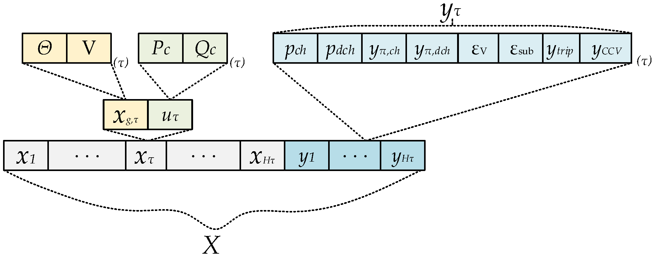
Figure 2 presents the described structure of the optimization variables. The fact that the auxiliary variables ( y τ ) are appended as last elements of vector X eases the extension of the stated problem. Additional objective terms might be assigned in the current formulation unless there is no dependence or conflicting interest upon the aforementioned objective.
The overall control scheme can be described by the set of Equations (13):
min u τ = 1 H t k N b [ c k ( τ ) ] T · u k , τ O 1 Δ τ + Φ p ,
subjected to
G j ( x τ , u τ , y τ ) = 0 j , τ N , T ,
H S u b ( x τ , u τ , y τ ) + ε s u b 0 i , τ J , T ,
V min ϵ V v j ( x τ ) V max + ϵ V i , τ N , T ,
h ξ ( x τ , u τ , y τ ) = 0 ξ , τ U , T ,
g ξ ( x τ , u τ , y τ ) 0 ξ , τ U , T ,
where vector [ c k ( τ ) ] T includes the price of each controllable unit per time step τ in €/kWh or €/kVArh. The constraints in (13a) set the nonlinear power flow equation at each bus of the network; inequality constraint (13b) poses the technical constraint for the MV/LV transformer; the boxed constraints in (13c) to respect all nodal voltages to range strictly within the admissible bounds. The additional positive variable ϵ V is used to relax the voltage constraints and avoid infeasibility. The latter is applicable substantially when the active measures are not adequate for addressing voltage problems. Accordingly, since a transformer is capable of being operated in full load conditions or slightly higher for a certain short interval, an auxiliary variable is also applied to turn these constraints less tight. Th constraints (13d)–(13e) correspond to the operational limits of the controllable DER.
In the following subsection, the resolution of the optimal control problem is analytically discussed through the optimization techniques used to address it efficiently. The proposed control scheme evidently deals with a large number of decision variables - X R N X : N X = ( 2 3 N b + 2 N c + 2 N B E S S + 2 N e v + 3 ) · H τ -. Accordingly, the power flow through the nonlinear equations are accounted N n o n l i n = 2 3 N b . Such large optimization problems, where the structure of the Jacobian of the nonlinear constraints present very sparse blocks, should possibly reveal particular framing of the problem re-structuring it and inherently leading to improved computational efficiency. In [37], the authors restructure the multi-period OPF to a tailored approach exploiting its particularities. Hereby, particular techniques are proposed to speedup the largeness of the nonlinear optimal control programming. The explicit calculation of the Jacobian and the Hessian is proposed, taking advantage of the sparsities, as well as slight pivotal elements to the Jacobian address any singularities met by the inter-temporal constraints. The initial point X 0 for the optimizer is either obtained through a local database which has stored previous occurrences or by running sequentially ( H τ ) power flows. Additionally, if load and weather forecasts fail to be obtained, a worst case scenario can be interrogated by a local historical database.

3.1. Interior-Point Primal-Dual Method for the Proposed Control Scheme

The proposed control scheme based on the MACOPF is stated with the set of Equation (13). Hereby, a discussion will follow based on an interior-point method, which follows the above form of the previous section, and will involve lengthy and complicated notation. To ease the description, the control problem is reformulated in a more compact manner (i.e., grouping the equalities and inequality constraints) as proposed in the literature [38,39,40]. Note that, with bold notation, a vector form is implied. The decision variables and state vectors are simply represented by one vector x :
min x f ( x ) ,
subject to
g E ( x ) = 0 ,
h I ( x ) 0 ,
x min x x max ,
where g E ( x ) contains any type of equality constraint (i.e., linear and nonlinear) and h I any type of inequality constraint. The inequalities constraints can be introduced as equality constraints by the addition of slack variables s j , such that h I ( x ) s = 0 . Then, a penalty function introduces a new form to the initial objective function as follows:
min x f p = f ( x ) μ ( k ) j = 1 N x n ( x j x j , min ) μ ( k ) j = 1 N x n ( x j , max x j ) μ ( k ) j = 1 N i n e q n ( s j ) ,
subject to
g E ( x ) = 0 , h I ( x ) + s = 0 , x , s 0 ,
where μ ( k ) is the the logarithmic barrier parameter for iteration k that essentially reduces monotonically to 0 as iteration progresses. The non-negativity conditions at (16) are handled by incorporating them into logarithmic barrier terms. The Lagrangian ( L p ) of the f p can be defined as:
L p ( x , λ , σ , s ) : = f p ( x ) λ T g E ( x ) σ T ( h I ( x ) + s ) L p ( x , λ , σ , s ) = f ( x ) μ ( k ) j = 1 N x n ( x j x j , min ) μ ( k ) j = 1 N x n ( x j , max x j ) μ ( k ) j = 1 N i n e q n ( s j ) λ T g E ( x ) σ T ( h I ( x ) + s ) ,
where vectors λ , σ are the Lagrange multipliers for the corresponding equality and inequality constraints. The first-order Karush–Kuhn–Tucker (KKT) condition (iff g E , h I are first order differentiable) for a local optimum point p = ( x , λ , σ , s ) are the following:
x L p ( x , λ , σ , s ) = x f p ( x ) λ x g E ( x ) T σ x h I ( x ) T D = 0 , μ L p = μ [ s ] 1 e λ = 0 , λ L p = g E ( x ) = 0 , σ L p = h I ( x ) s = 0 , D = μ [ x x min ] 1 e + μ [ x max x ] 1 e ,
where e is the appropriate size vector with all entries equal to one.
The first-order KKT conditions are necessary and sufficient for global optimality for a convex problem when the Linear Constraint Qualification (LICQ) holds [41]. In the proposed control scheme, the non-convex nature of the—exact—nonlinear power flow necessitates the verification second-order KKT conditions to certify the local optimality of p . The second-order conditions can be found analytically in the literature [38], since here the first-order will be analytically discussed due to the examination of linear dependence of the inter-temporal constraints introduced by DER.
The IP algorithm at iteration k requires the solution of the following nonlinear system:
x 2 L p x g E ( x ) x h I ( x ) 0 x g E ( x ) T 0 0 0 x h I ( x ) T 0 0 I 0 0 I s 2 L p Δ x Δ λ Δ σ Δ s = x f p ( x ) λ x g E ( x ) T σ x h I ( x ) T μ [ s ] 1 e λ g E ( x ) h I ( x ) s z x μ e .
The KKT system in Equation (19) is nonlinear and its solution most commonly in the literature [42] is addressed by applying the Newton’s method. In the proposed control scheme, the gradients for the nonlinear constraints and the Hessian of the Lagrangian are explicitly calculated. In case where these derivations are not provided, approximations based on finite differences are typically applied [43,44].

3.2. Gradients of Nonlinear Constraints and Hessian of Lagrangian

The gradient (see also Appendix B) of the objective function, the Jacobian of nonlinear constraints and Hessian of the Lagrangian are implicitly provided to the optimizer, by expanding the calculations presented in [45]. On this point, it is important to be stated that the voltage vectors are expressed using polar coordinates: expressing voltage in rectangular coordinates eliminates trigonometric functions from the PF equations [46]. Nevertheless, in [42,47], a benchmarked comparison of both types of coordinates present the same order of computational performance as well as an equivalent number of iterations for convergence for a typical OPF. On one hand, rectangular coordinates can ease the process of first and second order gradients leading to quadratic and constant forms; both types cannot avoid the nonlinear equalities (and inequality) constraints and form a convex region. Concurrently, rectangular coordinates may provide slightly faster evaluation of particular gradients and Hessian, but the voltage bounds are handled as functional bounds in many OPF problems.
Therefore, the complex voltage vector might be denoted by V R 3 N b . The element at bus j at phase a is υ j , a = | υ j , a | e j θ j , a . The derivation with the state vectors for instant period τ followed, obviously, for the other periods are 0 entries-:
V Θ τ = V τ Θ τ = j [ V τ ] V V τ = V τ V τ = [ V τ ] [ V τ ] 1 : = [ E ] .
The analytical AC power flow equations over all periods of the horizon window can be derived by the resolution of Equation (21). The operator ⊙ is used for element-wise matrix product. Complex number equations are not addressed by state-of-the art optimizers and only in a few cases yield faster solutions [48]. Thus, a segregation is proposed—as shown in Equation (22)—which introduces the power flows through the vector G ( X ) , due to their complex nature, which essentially cannot be posed at the optimization stage:
G c ( X ) = S b u s ( V ) + S d C g S g , G c : C n b C n b S b u s τ ( V τ ) = V τ ( I i n j τ ) = V τ ( Y b u s · V τ ) ,
G ( X ) = { G c ( X ) } { G c ( X ) } , G : R 2 n b R 2 n b .
The current bus injection I i n j appears in the power flow Equation (21). It would be useful for the power flow expressions derivation to present the corresponding for the current injections:
I i n j τ x τ = I i n j τ Θ τ I i n j τ V τ 0 0 , I i n j τ Θ τ = Y b u s V τ Θ τ = ( 20 ) j Y b u s [ V τ ] , I i n j τ V τ = Y b u s V τ V τ = ( 20 ) Y b u s [ E ] .
The first and second derivatives for the nonlinear constraints, which substantially refer to the power flow equation, will be based on the introduced vector G c ( X ) :
G X = G X = { G c ( X ) } X { G c ( X ) } X = G x 1 G x 2 G x H t G x H t G y 1 G y H t ,
G x τ = G Θ τ G v τ G P g τ G Q g τ .
The first order partial derivatives are presented for the defined G c , which can thereafter appended in Equation (25):
G c , Θ τ = S b u s ( V τ ) Θ τ = [ I i n j τ ] V τ Θ τ + [ V τ ] ( I i n j τ ) Θ τ = ( 20 ) j [ V τ ] [ I i n j τ ] Y b u s [ V τ ] ,
G c , V τ = S b u s ( V τ ) V τ = [ I i n j τ ] V τ V τ + [ V τ ] ( I i n j τ ) V τ = ( 20 ) [ V τ ] [ I i n j τ ] + Y b u s [ V τ ] [ V τ ] 1 ,
G c , P g τ = C g , G c , Q g τ = j C g ,
where ( C g ) N b × N c stands for the injection connectivity matrix that each element ( i , j ) is one if at bus i t h controllable asset j t h is connected, else the element is zero. It is obvious that the partial derivatives of G c ( x τ ) with respect to other x g , τ 2 , u g , τ 2 —with τ 2 τ —results in zero entries. The G X is therefore formed by two stacked matrices, which present sparse block diagonalities. The corresponding partial derivatives with respect to the auxiliary variables will be zero entries as well.
The second derivatives for the the complex power injections are necessary only for the assessment of the Hessian of the Lagrangian, which appears in iteration of the KKT-system—Equation (18). As it can be observed, the Hessian matrix of the Lagrangian can be given by Equation (1):
H p ( x , ) = X X L p = X X f ( X ) + X X g E ( λ ) + X X H ( X ) .
The second order derivatives for the complex power flows are calculated in proportion to the instant λ . The derivative is provided discretized in two parts:
2 G c λ x τ 2 = x τ λ G c , x τ T ( X ) = G c , Θ τ Θ τ G c , Θ τ V τ 0 0 G c , V τ Θ τ G c , V τ V τ 0 0 0 0 0 0 0 0 0 0 .
A brief presentation of all the subsequent expressions follows:
G c , Θ τ Θ τ = Θ τ j [ I i n j τ ] [ V τ ] Y b u s T [ V τ ] λ τ = [ V τ ] ( Y b u s ) T [ V τ ] [ λ τ ( Y b u s ) [ V τ ] λ τ A 1 + C 2 Y b u s [ V τ ] [ I b u s ] A 2 .
Accordingly, the G c , V τ Θ τ can be calculated as:
G c , V τ Θ τ = j B ( A 1 A 2 ) = ( G c , Θ τ V τ ) T ,
G c , VV τ = B ( C + C T ) B ,
where
B = [ V τ ] 1 , C 2 = [ λ τ ] [ V τ ] , C = C 2 ( Y b u s [ V τ ] ) .
The overall assessment of the second order gradient can be induced to a simple routine reducing computational effort and memory allocation by saving certain matrices presented above.
The subsequent gradients of the objective functions can be assessed for the proposed scheme since the f ( X ) = τ T f ( x τ ) substantially corresponds to a linear combination of convex functions. The first-order gradient of the objective will be comprised of constant and null entries since the costs are linear functions, as described in Section 3.5. By extension, the second-order derivatives of the objective function will be a null matrix.
If a solution of the barrier problem satisfies the primal-dual Equation (19) of the nonlinear KKT system, its solution may be approximated by an iteration of Newton’s method. The search direction can be obtained as a solution of the linearization of the KKT system, which is presented in Section 3.3.

3.3. Solution of Karush–Kuhn–Tucker Equations

Hereby, the barrier solution is presented for the optimal control problem (14), assuming that the decision variables x are positive (i.e., to avoid lengthy notation). The dual variables can be introduced as:
z i : = μ x i
H 0 J E T J I T I 0 [ λ ] 0 [ s ] 0 J E 0 0 0 0 J I I 0 0 0 z 0 0 0 [ x ] , ( k ) Δ x Δ s Δ λ Δ σ Δ z ( k ) = x L p λ L p σ L p s L p ,
where H = x x L p , J E = x g E ( x ) and J I = x h I ( x ) . The system (35) can be further simplified—based on Gaussian elimination—by eliminating the last row. Therefore, with this elimination, it will be:
H ^ 0 J E T J I T 0 [ λ ^ ] 0 I J E 0 0 0 J I I 0 0 ( k ) Δ x Δ s Δ λ Δ σ ( k ) = x L p + [ x ] 1 g E ( x ) s 1 ( μ e + s λ ) g E ( x ) h I ( x )
where H ^ = H k [ x k ] 1 [ z k ] and the diagonal matrix [ λ ^ ] = ( s k ) [ λ ] . The updates for the dual variables can be obtained from Equation (37):
Δ z k = [ x k ] 1 ( μ e [ z k ] Δ x k ) z k .
The overall resolution of the KKT system provides the search direction set for each subsequent iteration. An important condition for the Netwon step is that the Jacobian J E is a non-singular matrix. The latter implies properties which are assigned with the constraint qualification (CQ). The QP is a critical condition that needs to be assessed along with the KKT conditions. More analytically, the LICQ necessitates that the gradients of the equality constraints and any active bound constraints (i.e., binding constraints) which are linearly independent. If this does not hold, the KKT system cannot be resolved. In [41], the authors show that, for any local optimizer, the KKT conditions with LICQ satisfied can ensure the generic existence of the Lagrangian multipliers. The inter-temporal couplings among different periods τ in some cases lead to singularities for the Jacobian of the nonlinear equalities. Section 3.4 thoroughly discusses an efficient manner to avert such issues.

3.4. Intertemporal Couplings and Singular Jacobian

In the proposed multi-period OPF, the inclusion of inter-temporal constraints (e.g., mainly due to BESS and EVs) in most cases lead to the singularity of Jacobian matrix ( J E ). Whenever the gradients of the active constraints are linearly dependent, the consequence is that the Jacobian matrix for the first-order optimality conditions will be singular. This can be observed for the presented KKT systems (36) when there are some—assuming a set of j-binding constraints (from the h I inequalities) s j = 0 , while σ j 0 . Therefore, if additionally there are gradients of the respective gradients g E , h I are dependent when constraints are active the last three rows of the iteration matrix (36) will have dependent rows. An additional problematic condition might appear whether the binding conditions are linearly dependent; then, the Jacobi matrix is again singular according to [49].
The singularity issue to some extent occurs due to the structure of the control scheme, which essentially has no unique set of Lagrange multipliers corresponding to the dependent binding constraints. The particular case of BESS and the subsequent problems are analytically discussed in [49,50]. In these works, techniques are proposed to address the singularities; in [49], the authors simply suggest the elimination of the linearly dependent binding constraint on the Jacobian matrix is singular. Nonetheless, none can guarantee that the no constraint violation will take place and meanwhile it is tailored to mitigate certain singularities. The same authors propose further methods based on either a Moore–Penrose pseudoinverse of the Jacobian or by adding the standby losses.
Hereby, a simple technique will be presented which is model-free, which aims to correct the singularity introducing pivotal changes within the Jacobian matrix based on notions presented in [38]. To avoid the failure of singularity, a small pivot element (i.e., shadowed elements) might be added whenever the issue arises
H ^ 0 J E T J I T 0 [ λ ^ ] 0 I J E 0 δ π · I 0 J I I 0 0 ( k ) Δ x Δ s Δ λ Δ σ ( k ) = x L p + [ x ] 1 g E ( x ) s 1 ( μ e + s λ ) g E ( x ) δ π · λ h I ( x ) ,
where δ π stands for a fairly small positive number. The latter correction takes place in each iteration that the Jacobian is tracked as rank-deficient, which implies the linear dependency among constraints.

3.5. Inter-Temporal Costs

Inter-temporal costs have to be incorporated to ensure that transitions from one operating point to the next are feasible (i.e., managing flexibilities provided by the DER) and economical. These costs do apply independently to DER or assets while spanning multiple periods in particular, if multiple tariffs are defined along the horizon.
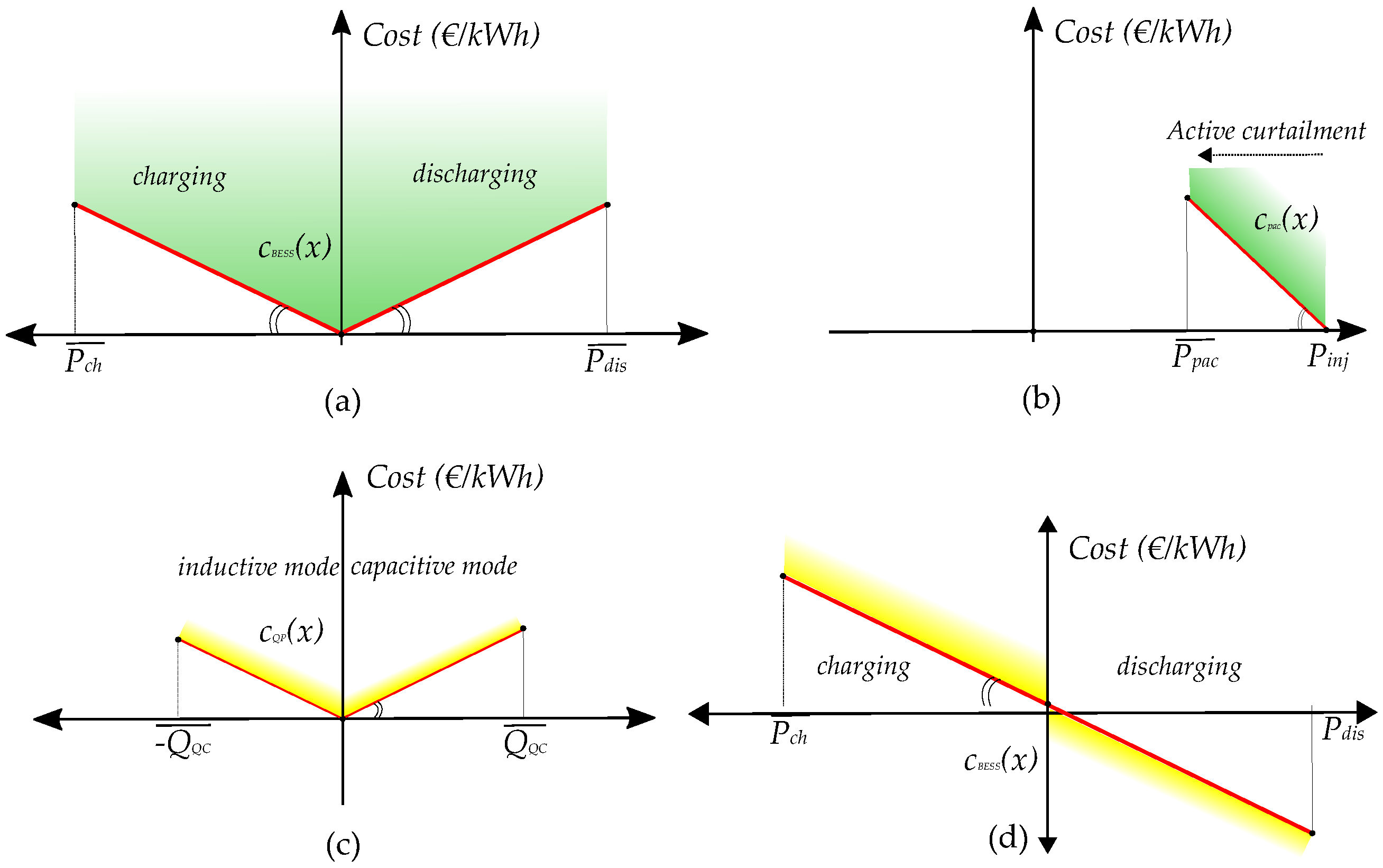
The costs for the controllable resources such as BESS and PVs follow a conditional operation regarding their mode of operation. The cost function, for instance, of charging a BESS is expressed by a linear convex function depending on the quantity of energy consumed—see the Figure 3a scenario when charging and discharging are equally priced. Any time step (e.g., charging or discharging) is dealt by imposing a Cost Constrained Variable (CCV) to represent the proper cost. The piecewise linear cost function c B E S S ( x ) —owned by the DSO—represented by the red line on Figure 3a—is substituted by an auxiliary variable y B E S S and a set of linear constraints. These linear constraints form a convex region with the c B E S S ( x ) , setting the y B E S S always to lie in the epigraph of the cost function. This auxiliary variable is onwards reflected to the objective function:
c B E S S ( x ) = π B E S S · x if x 0 ( discharging ) , π B E S S · x else x < 0 ( charging ) ,
where π B E S S corresponds to price of utilizing the BESS either for charging or discharging. The necessary linear constraints for the auxiliary variable are the following:
y B E S S π B E S S · x , y B E S S π B E S S · x .
Accordingly, the cost functions and their subsequent auxiliary variables are defined. Note that, for EV or domestic BESS, their cost function can have an arbitrage regime, in the sense that charging has a profitable impact on the objective function while discharging is penalizing it—Figure 3d. Note that all Figure 3 are indicative for a particular period τ ; different functions might be regarded for different time steps implementing demand response schemes based on variable pricing schemes.

4. Case Study Synopsis

The network selected as a case study to perform the validation of the proposed scheme belongs to the IEEE benchmarked LV European network [
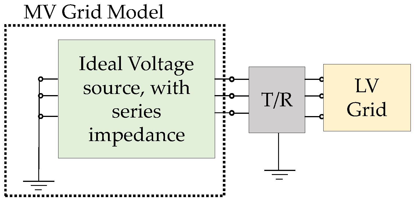
51]. The network corresponds to a real British low voltage feeder connected to the MV grid through a transformer of nominal power 800 kVA (
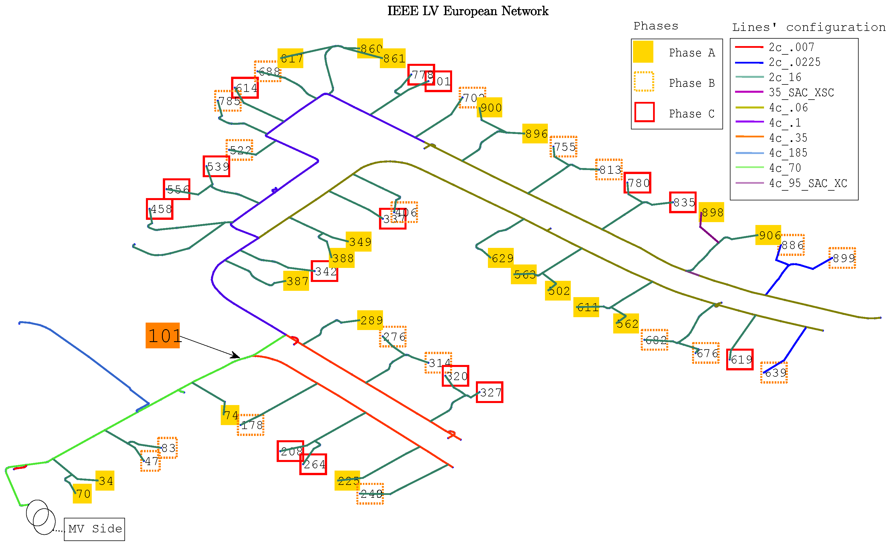
Figure 4). The transformer is modified and considered to be 20 kV to 400 V with nominal power of 150 kVA, since only one feeder is considered in the benchmark as well. The service cables to the 55 end-consumers are also included in the grid representation.
In all scenarios, a three-phase centralized BESS is assumed to be connected at node 101 (Figure 4). The BESS capacity is 90 kWh and the maximum charging and discharging rate is 45 kW. This BESS is assumed to have an initial SoC of 0.40 with S o C ̲ = 0.1 and, at the end of the optimization horizon, it has to be equal to the initial, S o C H τ = 0.40. The power factor of BESS 101 is considered as unitary for all the simulated cases and its charging and discharging efficiency is η c h , η d c h = 0.95, [52].
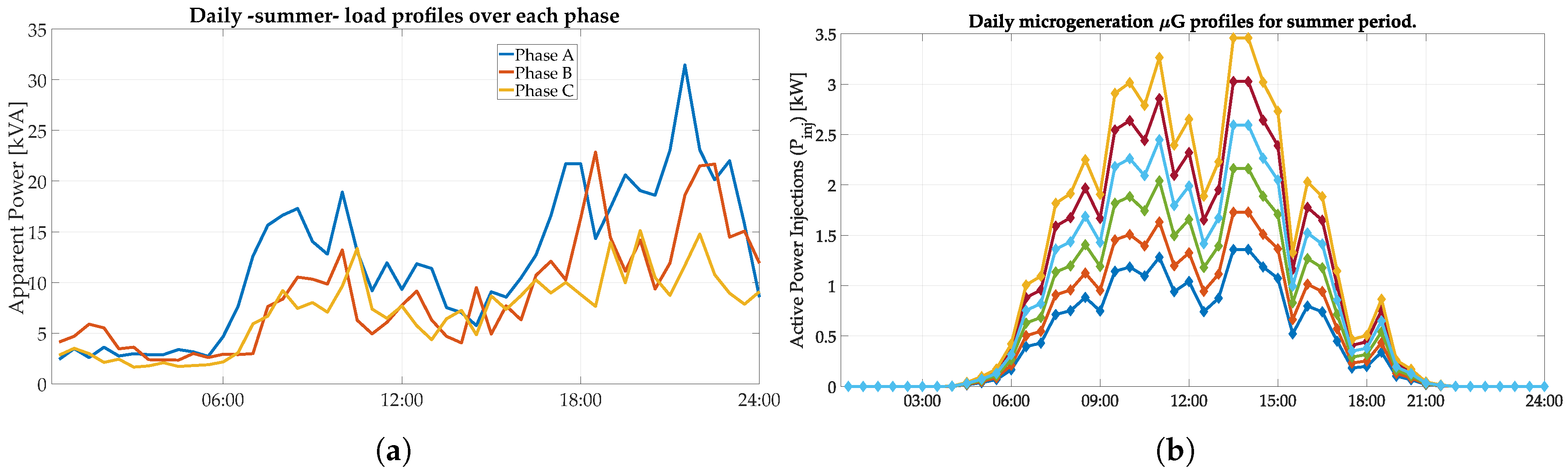
The load and the microgeneration profiles used correspond to daily data for a summer period, which are extrapolated from a realistic data pool provided for the benchmarked grid, which can be in [51]. All the consumers are single-phase and their phase connection is depicted in Figure 4. All the microgeneration units are considered as single-phase PV rooftop installations that are connected to the same phase as the respective residential user. The simulation day corresponds to a representative summer week day where typically peak loading conditions occur, where the load and generation profiles are illustrated in Figure 5a,b, accordingly.
Four EV models considered are based on four different EV models Nissan Leaf, Chevrolet Volt, BMW i3, Tesla S, which present different technical features regarding the Battery Capacity and charging power, in addition to their driving efficiency, which are considered from [53]. Their characteristics are listed in Table 1. All Tesla S and BMW i3 models are charged with an Efacec HomeCharger 7.4 kVA, while the rest of the EVs through an Efacec HomeCharger 3.4 kVA [54]. Therefore, the maximum charging power of each EV is limited and driven by the home charger used.
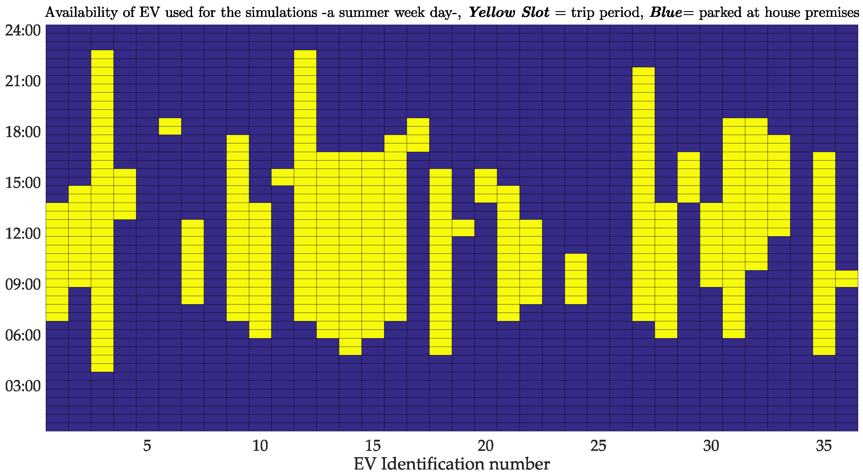
Concerning the EV usage, a routine is built to emulate credible scenarios, which are fed with public statistical data by [
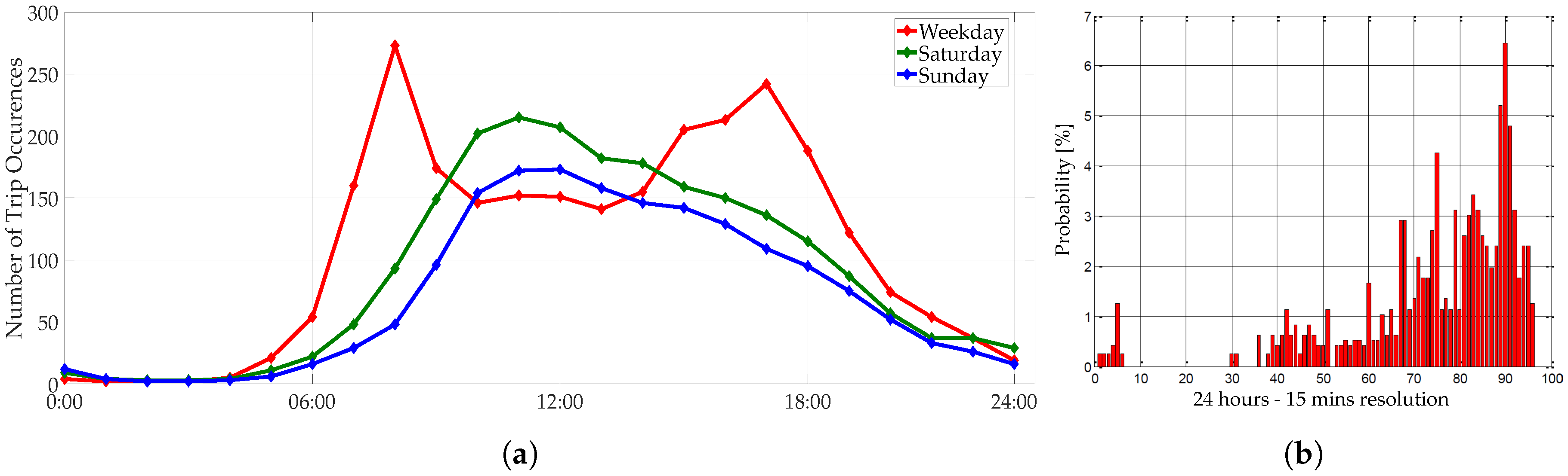
55]. This routine aims to capture patterns pertaining the EV usage upon different trip purposes as well as the trip duration (minutes) and length (km). The resulting data reflect a realistic response for the EV behavior during a day of operation, standing on the assertion that EVs charge exclusively at home. Nonetheless, the available statistical data do not explicitly provide information if the trip is from or to a destination. Therefore, the data as suggested in [56] are split into starting a trip and ending a trip, and it is assumed that a driver starts and ends every trip at home; hence, the cumulative data of trips for different days among different purposes are illustrated in Figure 6a. To assess the SoC change per each EV model used, averaged values for the purpose of each trip is used and correlated with each EV model’s driving efficiency (Table 1).
The following assumptions are also regarded for the EV:
  • Initial SoC for all EV models is S o C 0 = 0.5, which is meant to be the same at the end of the horizon S o C H τ = S o C 0 .
  • The charging efficiency and discharging—when V2G—efficiency are considered 85% for all EV models.
Two EV charging strategies are considered in this study:
  • “Dumb” charging or uncontrolled charging where the EVs are not incorporated within the proposed operational scheme. Such uncontrolled charing profiles are extracted using the data in probability density function presented in Figure 6b.
  • “Smart” charging, where the EV owner communicates relevant data (i.e., flexibility as defined above) regarding their commute and accordingly its availability to be charged according to the proposed tool. The V2G mode services enable the option to utilize the EV essentially for grid services. These constraints are automatically incorporated in the multiperiod-OPF scheme as the generalized set of Equations (13d)–(13e), whenever the availability of the EV allows it. The availability of the EV to charge is considered along the day during their idle periods (i.e., parked at the owner’s house).
Concerning the case where EVs follow the dumb charging, their charging occurs based on the distribution function given by [57]. The time departure and arrival as well as the daily distance traveled by each are randomly selected for a summer week day as presented in Figure 7.
According to the standard EN-50160, the 10 min mean r.m.s voltages shall not exceed the statutory limits during 95% of the week. Meanwhile, all 10 min mean r.m.s voltages shall not exceed the range of the Vn% + 10% and Vn% − 15% (which corresponds to 253 V and 195.5 V for most European grids). Given the fact that the proposed control scheme uses 30-min averaged data resolution, the voltage limits are set in [0.95, 1.05] p.u.values [58].
The percentage of PV and EV integration refers to the proportion of end users that own such units. For instance, 35% of EV penetration (i.e., 30 EVs), where the charging point of the EV are indicated in the last column of Table 1.
The use of DER is prioritized through the weighted terms c k ( τ ) , in the sense that the operational tool attempts to manage the flexibilities by addressing any voltage issues and respects the secondary transformer’s rated power with the controllable DER assigned with the more economical combination of c k ( τ ) . These c k ( τ ) can be attributed with real operational cost values to reflect monetary values for the use of flexibility. For this study, the weighted terms for the use of flexibility for each type of DER derive a merit order scheme settled as c B E S S < c E V < c V 2 G < c Q R < c A P C , which present respectively the price of using the BESS, incorporating an EV in the coordinated charging, the use of V2G mode and finally the use of reactive and active power by the microgeneration. In this way, the tool prioritizes the use of the centralized BESS that is owned by the DSO, avoids excessive active power curtailments, and the presence of the EVs restrains the dispatch of reactive power by the PVs, which is rather not effective for addressing voltage issues in LV grids (i.e., R > X ). Note that, in this study, the V2G operation is set slightly cheaper than any control of the microgeneration (i.e., APC or QR).
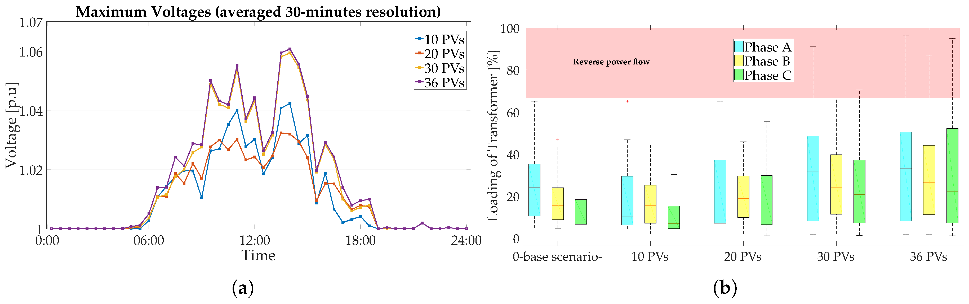
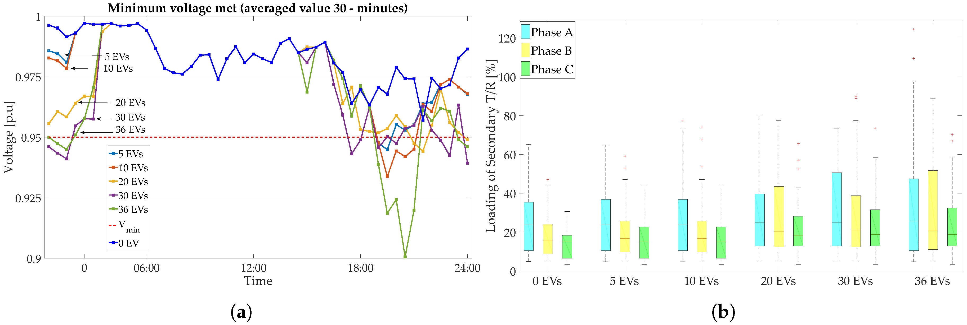
Prior to the presentation of the results within the proposed control approach, an exploration of discrete incremental integrations of PV and EV are given. For both cases, no control was deployed. In Figure 8a, the impact in voltage magnitudes is depicted; notable voltage drops can be observed for an EV integration about 35% (i.e., 20 EVs). Higher EV integration of 55–65% present severe voltage drops as well as the overloaded condition for the secondary substations (see Figure 8b). In Figure 9a, the analogous scenario for PV integration is presented. Overvoltages appear in scenarios with more than 35% of PV integration, where the reverse power flow towards the secondary substation can be also viewed through Figure 9b. One can notice that, in a mixed scenario with PVs and EVs, overvoltages will typically appear during morning and evening hours, whereas voltage sags will arise at late hours when most regular charging of EVs occur (see Figure 6a).
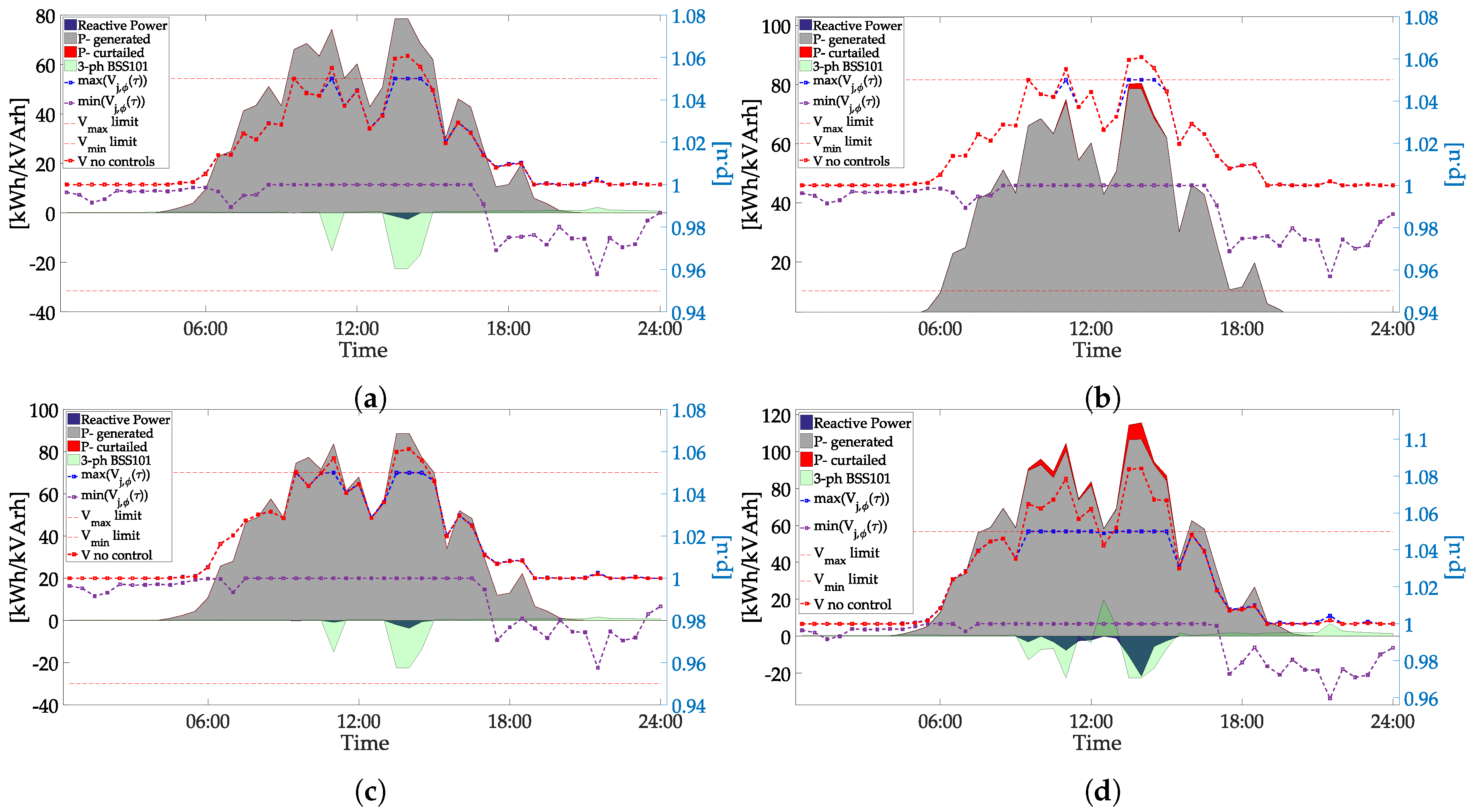
The explored scenarios in which the proposed control scheme is validated are defined in Table 2. Analytical information regarding the points of connection for the micro-generation and EVs are given in Appendix A. The scenarios are selected in order to validate that the MACOPF could allow high integration of microgeneration avoiding overvoltages and overloading of the transformer; secondly, mixed scenarios of DER integration including EVs are assessed by the coordinated control amongst them.

5. Results

The assessment of the proposed control framework takes places in all the scenarios for a day-ahead deterministic planning of operation with a time-step of Δ τ = 30 min, (i.e., 48 time steps). The available active measures for operational purposes are active power control of the centralized three-phase BESS, the coordinated charging of the EVs in addition to V2G mode of operation where both are considered once the EV is available (i.e., parked at house premises), and the control active and reactive power of the microgeneration. The setup for the controller considers minimum power factor for microgeneration 0.9 and maximum allowed curtailment 15% of the injected power by each unit.

5.1. Cases C01–C03

In scenario C01, with 65% (36 PV units) overvoltages (up to 1.062 p.u) do arise along the grid due to notable active power injections. Additionally, reversed power flow is also present, increasing the loading conditions of the secondary transformer up to about 90%. In Figure 10a, the actions taken along the horizon period are illustrated. Among the decisions, BESS 101 is essentially charged during sunny periods, reducing the reversed flows to the substation and restraining the voltages. Ultimately, the voltages issues are addressed in coordination with reactive power dispatch by the microgeneration (Figure 10a). Note that, for the same scenario, the use of the control approach solely with APC derives 5.3 kWh enabled, which corresponds to minimum curtailments since the controller is centralized (Figure 10b); hence, dealing with local P–V droop control would lead to higher curtailments since there is no topological confluence among PV and the decisions are merely based on the voltage at the point of connection of the inverter.
Scenario 02 refers to the point of PV integration where overvoltages and secondary substation are within admissible bounds without curtailing any active power by the PV units. The subsequent controls derived in this case refer to the coordinated operation of the centralized BESS with reactive power dispatch of a set of microgeneration units. The control setpoint of the BESS and its SoC for the day of operation are illustrated in Figure 11a–c.
Given the selected options for the controller (i.e., minimum PF = 0.9 and maximum APC 15%), the proposed control is capable of mitigating overvoltages and ensuring rated power for the secondary substation up to 85% of PV integration. Analytically, the actions taken for this scenario are illustrated in Figure 10d. Table 3 presents the anticipated curtailed power and dispatch reactive power within the day of operation for C01–C03.
Figure 12 presents all cases C01–C03 and the corresponding transformer loading conditions if the decision derived by the MACOPF are followed. It is noted that in all cases the MACOPF delivers actions which restrain the reversed power to the secondary substation. Only in scenario C03 is there a slight relaxation of the respective constraint since all of the active measures have been optimally utilized.
Excessive active power curtailment may indirectly mean high compensation costs for the DSO. The installation of a BESS can reduce the need of APC as shown in scenarios 01–03. In particular, scenario 01 presented that, solely based on APC, 5.3 kWh at least would be curtailed with local P–V droop based control. This fact may justify the investment from the DSO side when a high integration of PV prevails.
As a remark stands, the current analysis leans on averaged values of 30-min resolution; therefore, notable overvoltages may appear in higher resolution analysis for less PV integration. The latter justifies the tight limits posed for the voltage magnitudes for the purpose of this study. Concurrently, the importance of coordinated actions will be observable even in scenarios with less PV integration.

5.2. Cases C04–C06

In this part of the study, the EV integration is introduced within the LV grid. Initially, cases 04–05 examine the integration of 20 and 30 EV accordingly. The EV are randomly distributed along the end-consumers, only following the assumption that no more than one EV can be connected at each consumer. The point of connections for each scenario are given in Appendix A.
Case 04 presents voltage drops along the early hours (12:30 a.m. to 4:00 a.m.) but most significantly and below the posed lower limits in the late hours where the peak load is met (9:00 p.m.–10:00 p.m.). In this scenario, the MACOPF derives an optimal scheduling (Figure 13b) of the DSO’s BESS in order to address the undervoltages in the late hours. The coordinated charging for the current case is not deemed to be needed according to the proposed control. Nonetheless, it can be seen from Figure 13a that a slight increase of the peak load (i.e., hereby 6:30 p.m. to 11:00 p.m.) might trigger critical voltage sags and possible transformer loading conditions. It should be stressed that the 35% integration of EV, following dumb charging, leads to an increase of 22% of the peak load compared to the base case.
The following scenario C4 emulates a case with 55% of EV integration. In this case, the importance of multiple DER coordination is stressed since critical voltage sags can be noticed if EVs follow the dumb charging operation. The MACOPF yields a scheduling for the BESS 101 , which essentially supports during the late hours (i.e., 8:00 p.m.–9:30 p.m.) in addition to some EVs that are decided to operate in V2G mode. The peak load conditions along this interval are deteriorated due to the EVs that are added to consumption while returning from their trips. The coordinated charging during the early hours avoids the voltage drop along the distribution feeder, which would be noticed in the uncoordinated charging (Figure 14a).
The centralized BESS 101 is not adequate to entirely mitigate voltage problems due to the fact that some of the EVs are connected to the ending point of the feeder. Therefore, V2G mode of operation (i.e., for EVs that are willing to provide it) and coordinated charging efficiently added to the coordinated operation to maintain the voltages within the bounds. The SoC for all EVs are illustrated in Figure 14b. The V2G mode of operation comprises generally an effective measure to address undervoltages in LV grids due to the fact that active power is purely injected ( R > X ). Nevertheless, proper spatial and temporal distribution of the available EVs to provide such service is necessary. The spatial distribution refers to the bus and the phase of connection of the EV, whereas the temporal distribution to the availability along the horizon.
The following scenario C06 presents a case with increased PV and EV integration (i.e., 55% and 65%, respectively). The presence of PV installation injects notable active power during the sunny period (10:00 a.m. to 3:00 p.m.), whereas, in the rest of the time slots, voltage drops are observed due to the dumb charging. Notice that, in the current study, the PVs and EVs are randomly distributed, in the sense that a PV installation is not necessarily connected at a point where an EV is placed (see Table A1 and Table A2). In addition, the fact that the majority of EVs progress in the sunny hours essentially implies that only a few could be available to be shifted for charging in these time slots. The subsequent results for this case are illustrated in Figure 15a. In this scenario, as it can be seen from the SoC of EVs in Figure 15b, the EVs are charged within a coordinated way from 12:00 a.m. to 5:00 a.m. where light loading conditions prevail in the grid avoiding the undervoltages that are present within the dumb charging. Nonetheless, due to increased charging demand, idle EVs provide support at the slot 5:30 a.m. as well as at 5:00 p.m. to 6:00 p.m., maintaining the voltages within the bounds. Accordingly, during sunny periods, shifted EV charging can be noticed as well.

6. Conclusions

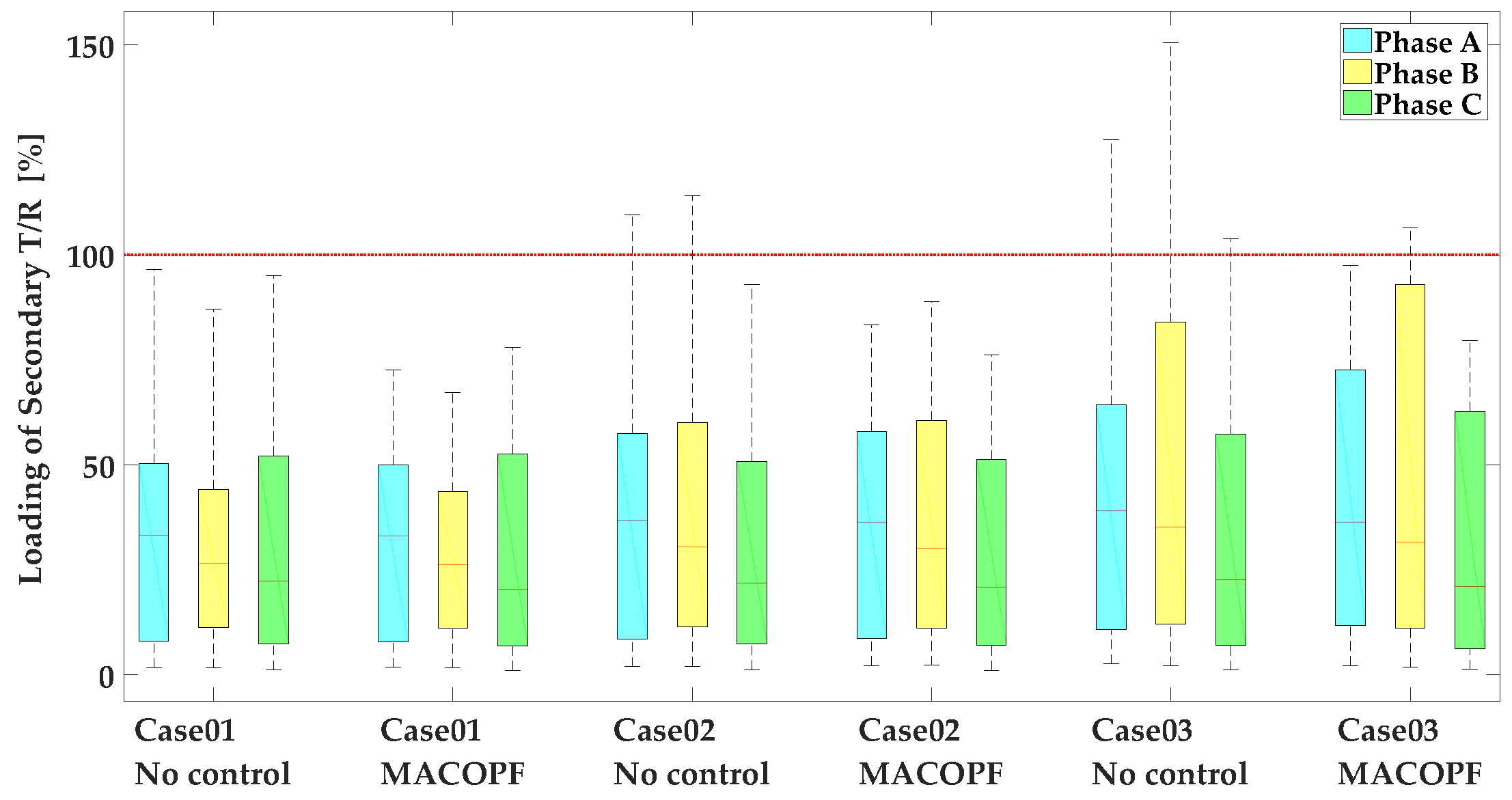
This work presents a tool that is capable of providing support to the DSO decision for the operation of LV three-phase distribution grids with increased integration of DER. The computational techniques proposed based on the explicit calculation of the first and second order derivatives (i.e., Jacobian and Hessian of the Lagrangian and the objective function), in addition to pivotal adjustments in the Jacobian, ensure a tractable optimal control based on the exact AC power flows.
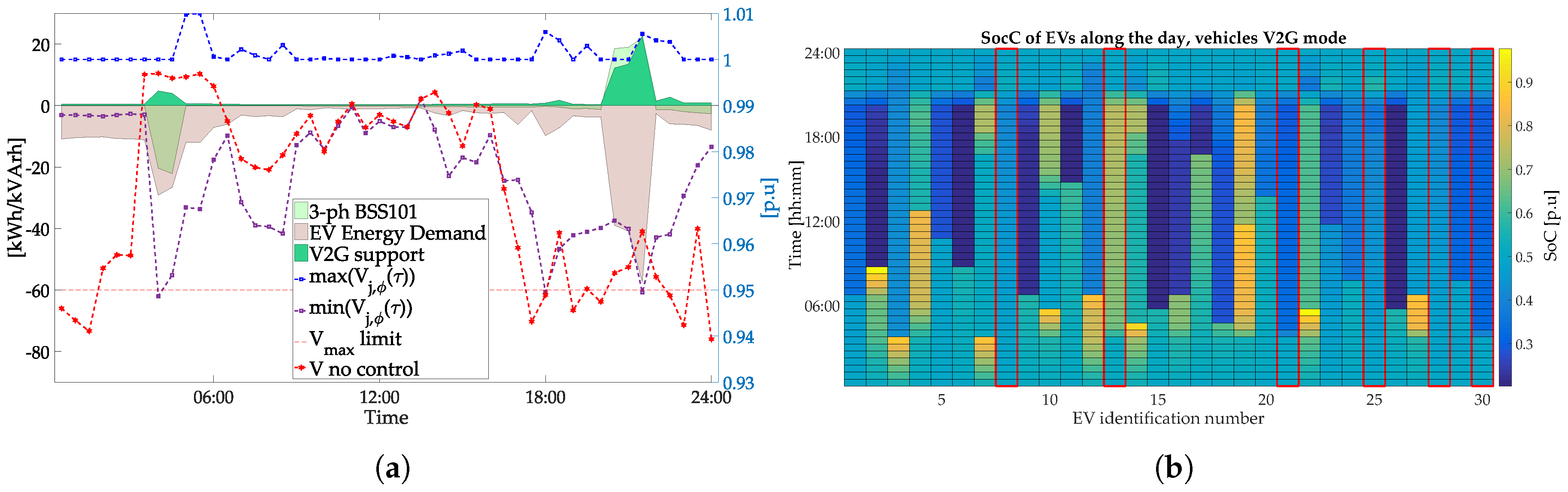
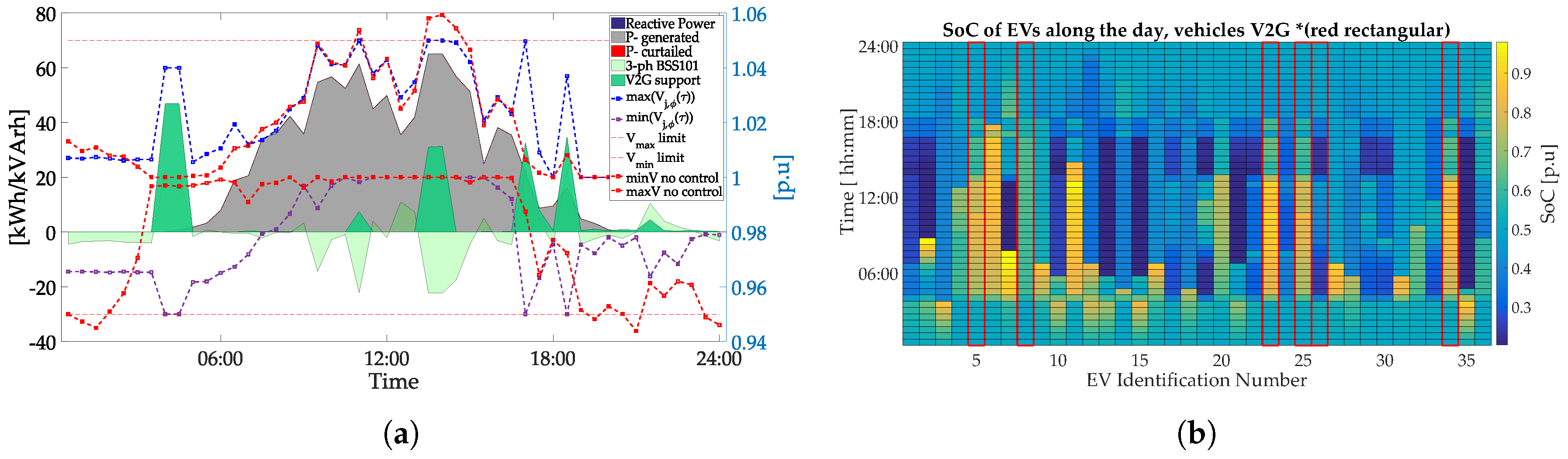
The proposed centralized scheme ensures admissible voltage profiles by minimizing the active power curtailments of microgeneration through the efficient coordination of DER—maximizing, in this sense, the integration of microgeneration. The coordinated operation among the DER units reassures in the presented study up to 73% integration of microgeneration avoiding any curtailment brought by PV units. The EV integration can be also maximized if coordinated charging is adopted within the MACOPF, which essentially can ensure admissible voltages and normal loading condition for the transformer. The V2G mode of operation can be regarded as important when a high integration of EV takes place with increased peak load conditions in the grid.
For all simulated cases, one can conclude that the radial configuration of LV networks present overvoltage issues particularly in buses—electrically—furthest from the substation since the high resistance of the lines leads to the aggravation of them. In addition, distant nodes at the ending point might face significant voltage drops (i.e., if EVs are present) or even overvoltages (i.e., if PVs are present). Therefore, the placement of a BESS in proper location (i.e., adjacent to nodes with voltage issues) along the grid is rather crucial since the installation adjacent to the secondary substation provides mainly reduced loading for the transformer rather than voltage support to the furthest points.
The proposed control scheme is based on deterministic analysis for the planning in a day-ahead scale for the operation of the grid. Meanwhile, the scheme can be deployed only by the subsequent communication technologies (for online implementation), together with forecasted data and power flow-state estimation tools (i.e., if topology is not known).

Author Contributions

Formal analysis, K.K.; Methodology, K.K.; Software, K.K.; Supervision, I.M., N.S. and H.L.; Validation, K.K.; Writing—original draft, K.K.; Writing—review & editing, I.M., N.S. and H.L.

Funding

This project has received funding from the European Unions Horizon 2020 research and innovation programme under the Marie Skodowska-Curie Grant No. 675318 (INCITE).

Conflicts of Interest

The authors declare no conflict of interest.

Abbreviations

The following abbreviations are used in this manuscript:
DERDistributed Energy Resources
LVLow Voltage
OPFOptimal Power Flow
PVPhotovoltaic
BESSBattery Storage System
EVElectric Vehicles
DSODistribution System Operator
A-DMSAdvanced Distribution Management Systems
CLControllable Loads
OLTCOn Load Tap Changer
MACOPFMultiperiod AC-OPF
IPInterior-Point
SoCState-of-Charge
V2GVehicle-to-Grid
APCActive Power Curtailment
QRReactive Power Control
BFSBackward-Forward Sweep
KKTKarush–Kuhn–Tucker
LICQLinear Constraint Qualification
CQConstraint Qualification
CCVCost Constrained Variable

Appendix A. Complementary Data for Case Study

Table A1. SPoints of PV Connections for the Presented Scenarios.
Points of PV
connections
522.2/388.1/178.2/
676.2/639.2/337.3/
701.3/614.3/562.1/
682.2/70.1/556.3/
629.1/47.2/349.1/
563.1/264.3/458.3/
249.2/289.1
611.1/74.1/320.3/
73.1/276.2/225.1/
327.3/387.1/619.3/
702.2
702.2/502.1/342.3/
208.3/539.3/
688.2/406.2
248.2/83.2/314.2/
896.1/785.2/900.1/
899.2/755.2/780.3/
898.1/813.2
Scenarios
[% of PV]
30%
55%
65%
85%
Table A2. Points of EV Connections for the Presented Scenarios.
Points of EV connections327.3/835.3/785.2/563.1/
755.2/249.2/225.1/47.2/
886.2/898.1/314.2/208.3/
906.1/861.1/320.3/682.2/
780.3/406.2/817.1/248.2
619.3/860.1/702.2/
458.3/899.2/264.3/
178.2/83.2/337.3/
556.3
73.1/349.1/701.3/
522.2/342.3/289.1
Scenarios [% of EV]30%
55%
65%

Appendix B. First and Second Order Derivatives for Multi-Variable Function

In this section, a brief description of the calculations of the first and second order gradients for the nonlinear constraints and the objective function. In general, for a scalar function f : R k R of a real vector X = [ x 1 , x 2 , , x k ] T , the Jacobian matrix that corresponds to the first-order derivatives is given as:
f X = f x 1 f x k .
The Hessian matrix of f that corresponds to the second-order derivatives is:
2 f X 2 = X f X T = 2 f x 1 2 f x 1 2 x k 2 f x k x 1 2 f x x k 2 .
For a vector function G : R k R m of a vector X, the first derivatives that form the Jacobian matrix is:
G X = G X = g 1 x 1 g 1 x k g m x 1 g m x k .

References

  1. Eid, C.; Codani, P.; Perez, Y.; Reneses, J.; Hakvoort, R. Managing electric flexibility from Distributed Energy Resources: A review of incentives for market design. Renew. Sustain. Energy Rev. 2016, 64, 237–247. [Google Scholar] [CrossRef] [Green Version]
  2. Lotfi, M.; Monteiro, C.; Shafie-khah, M.; Catalão, J.P.S. Evolution of Demand Response: A Historical Analysis of Legislation and Research Trends. In Proceedings of the 2018 Twentieth International Middle East Power Systems Conference (MEPCON), Cairo, Egypt, 18–20 December 2018; pp. 968–973. [Google Scholar] [CrossRef]
  3. Ochoa, L.F.; Mancarella, P. Low-carbon LV networks: Challenges for planning and operation. In Proceedings of the 2012 IEEE Power and Energy Society General Meeting, San Diego, CA, USA, 22–26 July 2012; pp. 1–2. [Google Scholar]
  4. Bruno, S.; La Scala, M. Unbalanced Three-Phase Optimal Power Flow for the Optimization of MV and LV Distribution Grids. In From Smart Grids to Smart Cities: New Challenges in Optimizing Energy Grids; Wiley: Hoboken, NJ, USA, 2016; pp. 1–42. [Google Scholar] [CrossRef]
  5. Control and Management Architectures. Smart Grid Handbook; Wiley: Hoboken, NJ, USA, 2016. [Google Scholar] [CrossRef]
  6. Karagiannopoulos, S.; Roald, L.; Aristidou, P.; Hug, G. Operational Planning of Active Distribution Grids under Uncertainty. Available online: http://eprints.whiterose.ac.uk/120043/ (accessed on 7 January 2018).
  7. Bruno, S.; Lamonaca, S.; Rotondo, G.; Stecchi, U.; La Scala, M. Unbalanced three-phase optimal power flow for smart grids. IEEE Trans. Ind. Electron. 2011, 58, 4504–4513. [Google Scholar] [CrossRef]
  8. Faria, P.; Spínola, J.; Vale, Z. Distributed Energy Resources Scheduling and Aggregation in the Context of Demand Response Programs. Energies 2018, 11, 1987. [Google Scholar] [CrossRef]
  9. Soares, T.; Silva, M.; Sousa, T.; Morais, H.; Vale, Z. Energy and Reserve under Distributed Energy Resources Management—Day-Ahead, Hour-Ahead and Real-Time. Energies 2017, 10, 1778. [Google Scholar] [CrossRef]
  10. Tonkoski, R.; Lopes, L.A.C.; El-Fouly, T.H.M. Coordinated Active Power Curtailment of Grid Connected PV Inverters for Overvoltage Prevention. IEEE Trans. Sustain. Energy 2011, 2, 139–147. [Google Scholar] [CrossRef]
  11. Weckx, S.; Gonzalez, C.; Driesen, J. Combined Central and Local Active and Reactive Power Control of PV Inverters. IEEE Trans. Sustain. Energy 2014, 5, 776–784. [Google Scholar] [CrossRef]
  12. Demirok, E.; González, P.C.; Frederiksen, K.H.B.; Sera, D.; Rodriguez, P.; Teodorescu, R. Local Reactive Power Control Methods for Overvoltage Prevention of Distributed Solar Inverters in Low-Voltage Grids. IEEE J. Photovolt. 2011, 1, 174–182. [Google Scholar] [CrossRef]
  13. Heleno, M.; Rua, D.; Gouveia, C.; Madureira, A.; Matos, M.A.; Lopes, J.P.; Silva, N.; Salustio, S. Optimizing PV self-consumption through electric water heater modeling and scheduling. In Proceedings of the 2015 IEEE Eindhoven PowerTech, Eindhoven, The Netherlands, 29 June–2 July 2015; pp. 1–6. [Google Scholar] [CrossRef]
  14. Olivier, F.; Aristidou, P.; Ernst, D.; Van Cutsem, T. Active Management of Low-Voltage Networks for Mitigating Overvoltages Due to Photovoltaic Units. IEEE Trans. Smart Grid 2016, 7, 926–936. [Google Scholar] [CrossRef]
  15. Degroote, L.; Renders, B.; Meersman, B.; Vandevelde, L. Neutral-point shifting and voltage unbalance due to single-phase DG units in low voltage distribution networks. In Proceedings of the 2009 IEEE Bucharest PowerTech, Bucharest, Romania, 28 June–2 July 2009; pp. 1–8. [Google Scholar] [CrossRef]
  16. Miranda, I.; Leite, H.; Silva, N. Coordination of multifunctional distributed energy storage systems in distribution networks. IET Gener. Transm. Distrib. 2016, 10, 726–735. [Google Scholar] [CrossRef]
  17. Fortenbacher, P.; Zellner, M.; Andersson, G. Optimal sizing and placement of distributed storage in low voltage networks. In Proceedings of the 2016 Power Systems Computation Conference (PSCC), Genoa, Italy, 20–24 June 2016; pp. 1–7. [Google Scholar] [CrossRef]
  18. Hoppmann, J.; Volland, J.; Schmidt, T.S.; Hoffmann, V.H. The economic viability of battery storage for residential solar photovoltaic systems—A review and a simulation model. Renew. Sustain. Energy Rev. 2014, 39, 1101–1118. [Google Scholar] [CrossRef]
  19. European Union. Directive 2009/72/EC of the European Parliament and of the Council of 13 July 2009 Concerning Common Rules for the Internal Market in Electricity and Repealing Directive 2003/54/EC. Off. J. Eur. Union 2009, 211, 55–93. [Google Scholar]
  20. Efkarpidis, N.; De Rybel, T.; Driesen, J. Optimization control scheme utilizing small-scale distributed generators and OLTC distribution transformers. Sustain. Energy Grids Netw. 2016, 8, 74–84. [Google Scholar] [CrossRef]
  21. Costa, H.M.; Sumaili, J.; Madureira, A.G.; Gouveia, C. A multi-temporal optimal power flow for managing storage and demand flexibility in LV networks. In Proceedings of the 2017 IEEE Manchester PowerTech, Manchester, UK, 18–22 June 2017; pp. 1–6. [Google Scholar] [CrossRef]
  22. Olival, P.C.; Madureira, A.G.; Matos, M. Advanced voltage control for smart microgrids using distributed energy resources. Electr. Power Syst. Res. 2017, 146, 132–140. [Google Scholar] [CrossRef]
  23. Madureira, A.; Gouveia, C.; Moreira, C.; Seca, L.; Lopes, J.P. Coordinated management of distributed energy resources in electrical distribution systems. In Proceedings of the 2013 IEEE PES Conference on Innovative Smart Grid Technologies (ISGT Latin America), Sao Paulo, Brazil, 5–17 April 2013; pp. 1–8. [Google Scholar] [CrossRef]
  24. Kotsalos, K.; Silva, N.; Miranda, I.; Leite, H. Scheduling of operation in Low Voltage distribution networks with multiple Distributed Energy Resources. In Proceedings of the CIRED Workshop, Ljubljana, Slovenia, 7–8 June 2018. [Google Scholar]
  25. Connell, A.O.; Flynn, D.; Keane, A. Rolling Multi-Period Optimization to Control Electric Vehicle Charging in Distribution Networks. IEEE Trans. Power Syst. 2014, 29, 340–348. [Google Scholar] [CrossRef]
  26. Campos, F.; Marques, L.; Kotsalos, K. Electric Vehicle CPMS and Secondary Substation Management. In Proceedings of the 8th Solar & 17th Wind Integration Workshop, Stockholm, Sweden, 16–17 October 2018. [Google Scholar]
  27. Efkarpidis, N.; De Rybel, T.; Driesen, J. Technical assessment of centralized and localized voltage control strategies in low voltage networks. Sustain. Energy Grids Netw. 2016, 8, 85–97. [Google Scholar] [CrossRef]
  28. Sperstad, I.B.; Marthinsen, H. Optimal Power Flow Methods and Their Application to Distribution Systems with Energy Storage: A Survey of Available Tools and Methods; SINTEF Energi. Rapport; SINTEF: Trondheim, Norway, 2016. [Google Scholar]
  29. Sereeter, B.; Vuik, K.; Witteveen, C. Newton Power Flow Methods for Unbalanced Three-Phase Distribution Networks. Energies 2017, 10, 1658. [Google Scholar] [CrossRef]
  30. Karagiannopoulos, S.; Aristidou, P.; Hug, G. Co-optimisation of Planning and Operation forActive Distribution Grids. In Proceedings of the 2017 IEEE Manchester PowerTech, Manchester, UK, 18–22 June 2017. [Google Scholar]
  31. Christakou, K.; Tomozei, D.C.; Le Boudec, J.Y.; Paolone, M. AC OPF in radial distribution networks–Part I: On the limits of the branch flow convexification and the alternating direction method of multipliers. Electr. Power Syst. Res. 2017, 143, 438–450. [Google Scholar] [CrossRef]
  32. Ciric, R.M.; Feltrin, A.P.; Ochoa, L.F. Power flow in four-wire distribution networks-general approach. IEEE Trans. Power Syst. 2003, 18, 1283–1290. [Google Scholar] [CrossRef] [Green Version]
  33. Cheng, C.S.; Shirmohammadi, D. A three-phase power flow method for real-time distribution system analysis. IEEE Trans. Power Syst. 1995, 10, 671–679. [Google Scholar] [CrossRef]
  34. Bazrafshan, M.; Gatsis, N. Comprehensive Modeling of Three-Phase Distribution Systems via the Bus Admittance Matrix. IEEE Trans. Power Syst. 2018, 33, 2015–2029. [Google Scholar] [CrossRef] [Green Version]
  35. Gorman, M.; Grainger, J. Transformer modelling for distribution system studies. II. Addition of models to Y/sub BUS/and Z/sub BUS. IEEE Trans. Power Deliv. 1992, 7, 575–580. [Google Scholar] [CrossRef]
  36. Shirmohammadi, D.; Hong, H.W.; Semlyen, A.; Luo, G.X. A compensation-based power flow method for weakly meshed distribution and transmission networks. IEEE Trans. Power Syst. 1988, 3, 753–762. [Google Scholar] [CrossRef]
  37. Kourounis, D.; Fuchs, A.; Schenk, O. Towards the Next Generation of Multiperiod Optimal Power Flow Solvers. IEEE Trans. Power Syst. 2018. [Google Scholar] [CrossRef]
  38. Nocedal, J.; Wright, S.J. Numerical Optimization, 2nd ed.; Springer: New York, NY, USA, 2006; pp. 497–528. [Google Scholar]
  39. Zhu, J. Optimization of Power System Operation; John Wiley & Sons, Inc.: Hoboken, NJ, USA, 2015; pp. 1–12. [Google Scholar] [CrossRef]
  40. Wachter, A. An Interior Point Algorithm for Large-Scale Nonlinear Optimization with Applications in Process Engineering. Ph.D. Thesis, Carnegie Mellon University, Pittsburgh, PA, USA, 2003. [Google Scholar]
  41. Hauswirth, A.; Bolognani, S.; Hug, G.; Dörfler, F. Generic Existence of Unique Lagrange Multipliers in AC Optimal Power Flow. arXiv, 2018; arXiv:1806.06615. [Google Scholar] [CrossRef]
  42. Torres, G.L.; Quintana, V.H. An interior-point method for nonlinear optimal power flow using voltage rectangular coordinates. IEEE Trans. Power Syst. 1998, 13, 1211–1218. [Google Scholar] [CrossRef]
  43. Wächter, A.; Biegler, L.T. On the implementation of an interior-point filter line-search algorithm for large-scale nonlinear programming. Math. Program. 2006, 106, 25–57. [Google Scholar] [CrossRef]
  44. Coleman, T.; Branch, M.A.; Grace, A. Optimization toolbox. In For Use with MATLAB. User’s Guide for MATLAB 5, Version 2, Relaese II; MATLAB, MathWorks: Natick, MA, USA, 1999. [Google Scholar]
  45. Zimmerman, R.D. AC Power Flows, Generalized OPF Costs and Their Derivatives Using Complex Matrix Notation; Report; PSERC: Tempe, AZ, USA, 2010. [Google Scholar]
  46. Frank, S.; Rebennack, S. An introduction to optimal power flow: Theory, formulation, and examples. IIE Trans. 2016, 48, 1172–1197. [Google Scholar] [CrossRef]
  47. Wood, A.J.; Wollenberg, B.F.; Sheblé, G.B. Power Generation, Operation, and Control, 3rd ed.; John Wiley & Sons: Hoboken, NJ, USA, 2013; book section 8. [Google Scholar]
  48. Gilbert, J.C.; Josz, C. Plea for a Semidefinite Optimization Solver in Complex Numbers. Available online: https://hal.inria.fr/hal-01497173/document (accessed on 28 January 2018).
  49. Baker, K.; Hug, G.; Xin, L. Inclusion of inter-temporal constraints into a distributed Newton-Raphson method. In Proceedings of the 2012 North American Power Symposium (NAPS), Boston, MA, USA, 4–6 August 2011; pp. 1–6. [Google Scholar] [CrossRef]
  50. Baker, K.; Zhu, D.; Hug, G.; Li, X. Jacobian singularities in optimal power flow problems caused by intertemporal constraints. In Proceedings of the 2013 North American Power Symposium (NAPS), Manhattan, KS, USA, 22–24 September 2013; pp. 1–6. [Google Scholar] [CrossRef]
  51. Espinosa, A.N. Dissemination Document “Low Voltage Networks Models and Low Carbon Technology Profiles”; The University of Manchester: Manchester, UK, 2015. [Google Scholar]
  52. Palizban, O.; Kauhaniemi, K. Energy storage systems in modern grids—Matrix of technologies and applications. J. Energy Storage 2016, 6, 248–259. [Google Scholar] [CrossRef]
  53. Osório, G.; Shafie-khah, M.; Coimbra, P.; Lotfi, M.; Catalão, J. Distribution system operation with electric vehicle charging schedules and renewable energy resources. Energies 2018, 11, 3117. [Google Scholar] [CrossRef]
  54. Efacec. EV Homecharger. Available online: http://electricmobility.efacec.com/wp-content/uploads/2016/10/CS195I1404C1_HC.pdf (accessed on 16 November 2018).
  55. Survey, N.T. National Travel Survey: England 2016; Report; National Travel Survey: Great Britain, UK, 2016.
  56. Pedersen, R.; Sloth, C.; Andresen, G.B.; Wisniewski, R. DiSC: A simulation framework for distribution system voltage control. In Proceedings of the 2015 European Control Conference (ECC), Linz, Austria, 15–17 July 2015; pp. 1056–1063. [Google Scholar]
  57. Richardson, P.; Moran, M.; Taylor, J.; Maitra, A.; Keane, A. Impact of electric vehicle charging on residential distribution networks: An Irish demonstration initiative. In Proceedings of the 22nd International Conference and Exhibition on Electricity Distribution (CIRED 2013), Stockholm, Sweden, 10–13 June 2013; Volume 2013, pp. 1–4. [Google Scholar] [CrossRef]
  58. Masetti, C. Revision of European Standard EN 50160 on power quality: Reasons and solutions. In Proceedings of the 2010 14th International Conference on Harmonics and Quality of Power (ICHQP), Bergamo, Italy, 26–29 September 2010; pp. 1–7. [Google Scholar]
Figure 1. Configuration for interconnection of MV with the LV grid.
Energies 12 01182 g001
Figure 2. Structure of optimization variables; discriminated by state vector, control variables and the auxiliary variables per each time step.
Energies 12 01182 g002
Figure 3. Cost function functions. (a) cost function for utilizing a BESS-owned by the DSO; (b) cost of active power curtailment; (c) cost function of reactive power control for microgeneration; (d) cost function of an EV with V2G operation.
Energies 12 01182 g003
Figure 4. The IEEE European LV benchmark network. Fifty-five consumers are connected to this case network.
Energies 12 01182 g004
Figure 5. Data profiles: (a) load profiles; and (b) micro-generation profiles using seasonal (e.g., summer profiles) and regional data.
Energies 12 01182 g005
Figure 6. Data profiles: (a) trips in progress along a week. and (b) probability density function for EV charging demand, used for the dumb charging scenarios (source: [57]).
Energies 12 01182 g006
Figure 7. State of the trip for Electric Vehicles used along the simulation period. Profiles were extracted for a summer week day.
Energies 12 01182 g007
Figure 8. Incremental integration of EV scenarios: (a) minimum voltage range over all phases and buses and (b) secondary transformer loading for each case of EV integration (the increase in loading is observed up to 120%).
Energies 12 01182 g008
Figure 9. Incremental integration of EV scenarios: (a) minimum voltage range over all phases and buses and (b) secondary transformer loading for each case of EV integration (the increase in loading is observable up to 120%).
Energies 12 01182 g009
Figure 10. Incremental integration of PV, Cases 01–03: (a) Case 01; (b) Case 01, solely APC was selected within the controller; (c) Case 02; (d) Case 03.
Energies 12 01182 g010
Figure 11. Control set-points and SoC derived by the MACOPF for centralized three-phase BESS 101 for: (a) Case 01; (b) Case 02; (c) Case 03.
Energies 12 01182 g011
Figure 12. Secondary transformer loading conditions for Cases 01–03, overloaded conditions are noticed due to reversed power injected by microgeneration units; admissible conditions are obtained applying the proposed coordinated operation.
Energies 12 01182 g012
Figure 13. Case 04: (a) resulting voltage ranges and actions yielded for BESS 101 ; (b) control set-points and SoC for BESS 101 .
Energies 12 01182 g013
Figure 14. Case 05: (a) resulting voltage ranges, coordinated charging in comparison with dumb charging; BESS 101 scheduling of operation and V2G actions; (b) SoC for all EVs; circled by red line correspond to V2G mode of operation.
Energies 12 01182 g014
Figure 15. Case 06: (a) resulting voltage ranges, coordinated charging in comparison with dumb charging; BESS 101 scheduling of operation and V2G actions; (b) SoC for all EVs, circled with a red line, correspond to V2G mode of operation.
Energies 12 01182 g015
Table 1. Electric Vehicles’ models and characteristics.
EV ModelBattery Capacity
[kWh]
Charging Power
[kW]
Driving Efficiency
(km/kWh)
End-User Owner
Nissan Leaf2446.7249.2/861.1/264.3/522.2
Chevrolet Volt163.753.75327.3/755.2/886.2/906.3/780.3/
619.3/899.2/337.3/701.3
BMW i322117.2785.2/225.1/314.2/320.3/
817.3/702.2/178.2/73.1/342.3
Tesla S60116.7563.1/47.2/208.3/682.2/406.2/
248.2/458.3/83.2/349.1/289.1
Table 2. Scenarios’ description.
ScenarioCase 01 (C1)Case 02 (C2)Case 03 (C3)Case 04 (C4)Case 05 (C5)Case 06 (C6)
EV [%]000355565
PV [%]5573850055
BESS 101
Table 3. Resulting curtailed active power and dispatched reactive power for the microgeneration units.
ScenarioCurtailed Energy
[kWh]
Reactive Energy
[kVArh]
Case 0103.94
Case 0207.43
Case 0334.559.3

