Estimating On-Road Vehicle Fuel Economy in Africa: A Case Study Based on an Urban Transport Survey in Nairobi, Kenya

Abstract

In African cities like Nairobi, policies to improve vehicle fuel economy help to reduce greenhouse gas emissions and improve air quality, but lack of data is a major challenge. We present a methodology for estimating fuel economy in such cities. Vehicle characteristics and activity data, for both the formal fleet (private cars, motorcycles, light and heavy trucks) and informal fleet—minibuses (matatus), three-wheelers (tuktuks), goods vehicles (AskforTransport) and two-wheelers (bodabodas)—were collected and used to estimate fuel economy. Using two empirical models, general linear modelling (GLM) and artificial neural network (ANN), the relationships between vehicle characteristics for this fleet and fuel economy were analyzed for the first time. Fuel economy for bodabodas (4.6 ± 0.4 L/100 km), tuktuks (8.7 ± 4.6 L/100 km), passenger cars (22.8 ± 3.0 L/100 km), and matatus (33.1 ± 2.5 L/100 km) was found to be 2–3 times worse than in the countries these vehicles are imported from. The GLM provided the better estimate of predicted fuel economy based on vehicle characteristics. The analysis of survey data covering a large informal urban fleet helps meet the challenge of a lack of availability of vehicle data for emissions inventories. This may be useful to policy makers as emissions inventories underpin policy development to reduce emissions.

1. Introduction

One approach to mitigating the impacts of air pollution on human health, and impacts of greenhouse gases (GHGs) on climate, is to reduce the growth of vehicle fuel consumption by improving fuel economy [1,2,3,4,5,6]. Since fuel economy is a good indicator of GHG emissions it has become an important metric to assess trends and allow comparisons in GHG emissions between different vehicles as well as between vehicle fleets from different world regions. It is also a key indicator by which vehicle manufacturers assess compliance with GHG emission targets. As such, making reliable assessments of fuel economy for in-use vehicle fleets is an important policy tool for helping to target emission reduction policy [6].

Globally, governments have developed and implemented fuel economy policy and standards that specifically target fuel consumption to reduce GHGs. Such policies and standards, have been implemented in four of the largest vehicle markets: USA, China, EU, and Japan [1,6,7,8]. Policies and standards in other major global markets (Australia, Brazil, India, Mexico and South Korea) tend to harmonize with these larger markets [6]. Typically, these vehicle manufacturers declare fuel economy for new vehicles determined by chassis dynamometer testing of representative vehicles under laboratory conditions [8,9]. However, there is usually a discrepancy between laboratory tests and on-road values as laboratory conditions cannot reflect real-world driving conditions during a vehicle’s lifetime [6,8,9,10,11,12,13]. Furthermore, the underestimation of actual fuel economy in laboratory type-approval testing directly affects achievable GHGs reductions [14]. Measuring on-road fuel economy has been undertaken using portable emission measuring monitoring systems (PEMS), but this is expensive and time consuming as measurements are only provided for a single vehicle over a short time period [9]. Therefore, real-world fuel efficiency emission data are often lacking, especially in developing countries [10,15].

Estimating fleet fuel economy of in-use vehicles is difficult as it varies with a number of other factors such as: the number of vehicles, fleet composition, vehicle characteristics, vehicle activities, fuel type and quality, congestion, driving style, road type, inspection and maintenance and degradation [16,17]. Prior studies have noted the importance of determining in-use fleet fuel economy especially with vehicles with accumulated mileage over 500,000 km [18,19]. USA and European environmental agencies factor in deterioration rates for vehicles under this mileage, but engines now last over 800,000 km before requiring the first rebuild of the engine [19]. These very high mileages are typical in vehicle fleets in Africa, and the costliness of studies and limited resources are even more of a hindrance when determining in-use fuel economy. Where these data are available, they can be used to estimate current GHG emissions, establish baseline emissions and explore future emission scenarios for a changing vehicle fleet. As such, knowledge of current emissions is crucial to the development and implementation of emission reduction policy measures which are currently lacking in Africa [20]. In addition, lack of vehicle activity data in formulating Intended Nationally Determined Contribution (INDC) for the transport sector [21], as set out by United Nations Framework Convention on Climate Change mitigation [22], has been identified by national governments in Africa as a major challenge in determining priorities in transport mitigation options.

To estimate in-use fuel economy of a vehicle fleet in a typical sub-Saharan African (SSA) city such as Nairobi, one needs data to describe the fleet composition, characteristics and activity for in-use vehicles. Moreover, these data need to include the total number of vehicles disaggregated by vehicle type, fuel type, age, emission technology and annual mileage (i.e., vehicle kilometres travelled (VKT) per year [23,24,25]. These data may be found in vehicle registries but these are often incomplete, inaccurate, inconsistent and outdated in developing countries [7,9,10]. Often national vehicle registries do not portray actual vehicle distribution on city roads, for example, vehicles registered in Nairobi may be in circulation elsewhere [26]. A particular challenge arises from the growing use of informal transport in SSA such as the use of matatus [27,28,29], bodabodas [30,31] and tuktuks [32]. These vehicles tend to be unregistered (making it difficult to use standard fleet inventory methods to capture their contribution to urban traffic) as well as being old, poorly maintained and overloaded during use, all factors that will increase tail-pipe emissions resulting in enhanced air pollution [32,33]. Therefore, in SSA the high composition of such vehicle fleets may be a source of uncertainties [34]. Thus, developing methodologies that can capture this unique but important component of the vehicle fleet in SSA cities is crucial for the development of representative assessments of the contribution of the transport sector to the atmospheric pollution burden. To address these data shortages, traffic video and parking lot surveys are often conducted and these data used as input for traffic models [23,24,25,34,35]. These types of survey however, face various challenges, for example, in determining VKT, type of vehicle, age and emission technologies on the vehicle [35,36,37]. To overcome some of these challenges, previous studies in Nairobi, have made certain assumptions which no longer hold, such as, the belief that licence plate data may serve as a proxy for the age and mileage of the vehicle [37].

Mathematical models for predicting fuel economy have been developed using vehicle physical characteristics such as engine size, maximum vehicle power, vehicle torque, vehicle weight, wheelbase and cross-sectional area [38,39,40]. The development of one such model required a large detailed historical dataset of new light duty vehicles, n = 6246, with highway fuel economy data and corresponding vehicle characteristics [39]. In that study, the fuel economy was assumed to be as declared by the manufacturers as per corporate average fuel economy (CAFÉ) standards. This level of quality and quantity of data is rarely available, especially for developing countries [41]. Furthermore, the fuel economy declared for new vehicles is extremely unlikely to be transferable to the majority of the in-use, often old and second-hand, vehicle fleet in developing countries [42].

Vehicle fuel economy and consumption are terms that are often used interchangeably in the literature [5,6,8,14,39,43,44,45,46]. Within this study, fuel economy will refer to volume of fuel consumed per distance (L/100km) and fuel consumption will refer to volume of fuel consumed over time (L/day). Kenya does not have fuel economy standards [21]. A previous study estimated Kenyan fuel economy to be near equivalent to European and Japanese standards lagged by 8 years [47]. In that study an assumption was made in the absence for in-use vehicle activity data for the Kenyan fuel economy fleet to be equivalent to European fleets of the same year of manufacture; in addition, the study only covered light-duty newly registered vehicles.

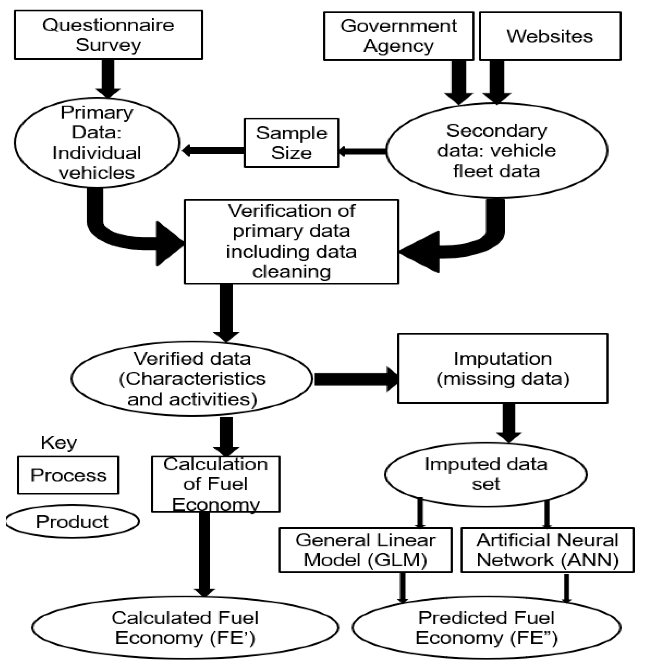
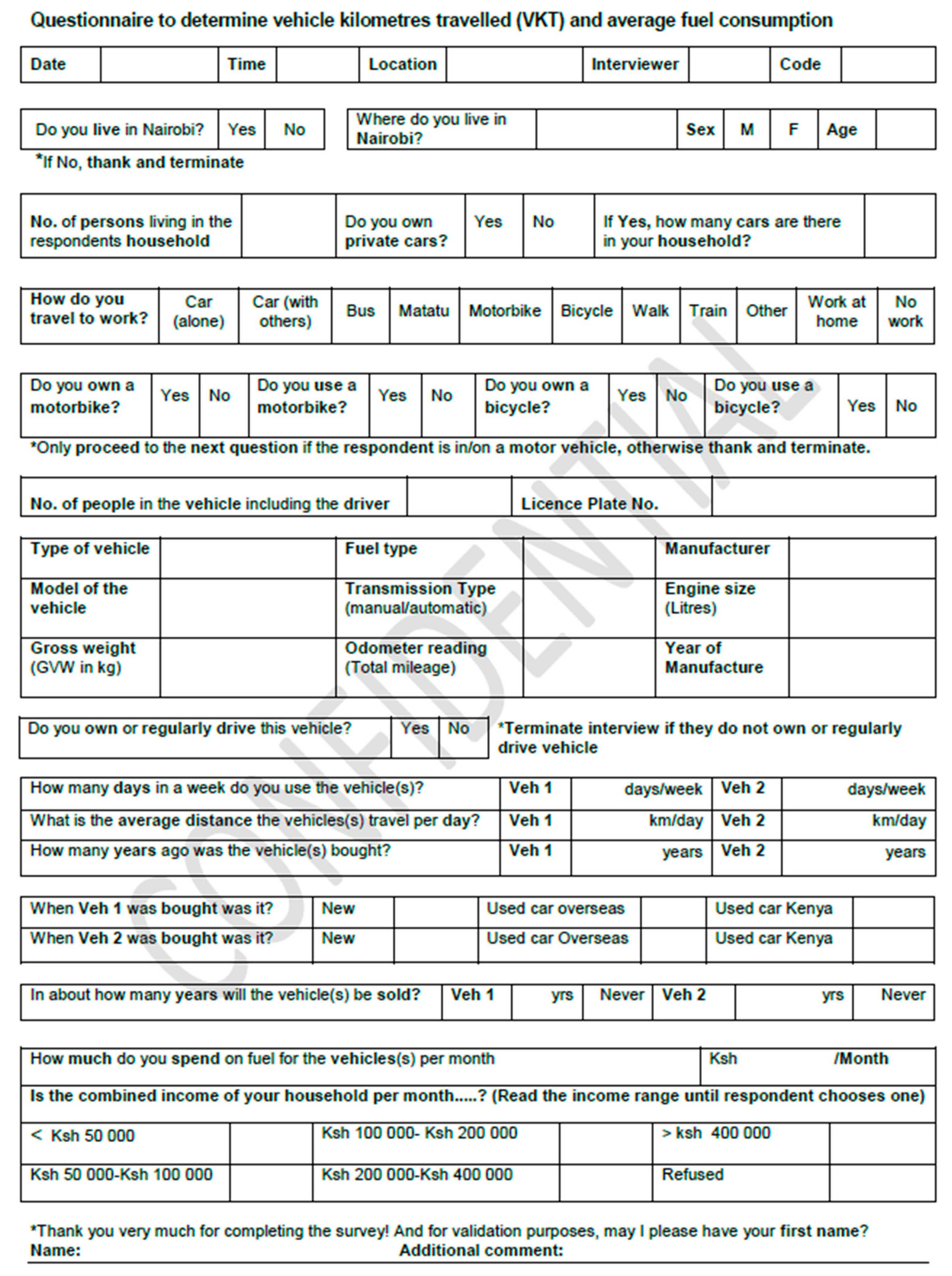
The overall objective of this paper is to develop a vehicle fleet questionnaire survey and associated procedure whose applicability is demonstrated for Nairobi Metropolitan Region (NMR), Kenya, allowing for the collection of primary data that includes characteristics such as engine size, weight of vehicle, mileage, money spend on fuel, transmission, age of vehicle, fuel type and vehicle utility. These primary data (mileage and the money spend on fuel) are used to calculate fuel economy. We also use a statistical method, multiple imputation, to deal with missing data [48], a common problem with surveys. To the authors’ knowledge, this approach for dealing with missing data has not previously been applied in vehicle survey data. The secondary data, obtained from existing literature, are used to determine the total number and composition of vehicles as well as to verify primary data describing vehicle characteristics. These verified primary data, when used in conjunction with secondary data, gives a baseline of real-world vehicle characteristics and activity for in-use vehicles. Further, this paper demonstrates how to use previously applied methodologies to build mathematical models to predict fuel economy; here we use and compare generalized linear models (GLM) and artificial neural networks (ANNs) [39,49]. These methods have the potential to be rapidly deployed in other SSA cities and regions which suffer from similar data limitations and resources and importantly can capture the variability in the vehicle activity and emission data that exists both in the formal and informal vehicle fleets.

2. Materials and Methods

Nairobi and the larger NMR was chosen as the site of the study as Nairobi is a typical SSA city in terms of socioeconomic status, size and population growth [50]. Figure 1 describes the data combinations required to develop the NMR vehicle fleet dataset and how this is then used to estimate fuel economy using the three different modelling approaches: calculated fuel economy, GLM and ANN. The modelling approaches used to estimate in-use fuel economy (FE) for the on-road vehicle fleet in Nairobi require data describing vehicle characteristics and vehicle activity as listed in Figure 1. Primary data were collected using a questionnaire survey (see Appendix A Figure A1). Secondary data were used to determine the total number of vehicles and fleet composition as well as to verify the fleet compositions and characteristics derived from the questionnaire survey primary data collection (i.e., vehicle characteristics: vehicle weight, engine size).

2.1. Secondary Databases

The total number of vehicles and fleet composition for vehicles in Kenya were obtained from the Kenya National Bureau of Statistics (KNBS) [51]. The composition of the vehicles in NMR were obtained from a transport feasibility surveys [52,53]. Vehicle registration data for all light duty vehicles in Kenya from 2010–2012 were obtained from a global fuel economy initiative (GFEI) between the Partnership for Clean Fuels and Vehicles (PCFV) of United Nations Environment Program (UNEP) and the Energy Regulatory Commission of Kenya (ERC) [47]. Data describing the total number of vehicles was used to determine the sample size required for the questionnaire survey. The NMR fleet composition was used to determine the sample weighting of the different vehicle categories for the field survey.

2.2. Questionnaire Survey

A questionnaire-based quantitative vehicle fleet survey was developed to collect data for the 18 variables describing vehicle characteristics and vehicle activity and trialled in Nairobi (see

Table 1. 18 variables identified from questionnaire survey data divided into two categories: numerical data and categorical data.

Numerical Data	Categorical Data
Unique vehicle identifier code	Type of vehicle
Engine size (cc)	Fuel type
Gross vehicle weight (kg)	Manufacturer
Odometer reading	Model
Year of vehicle manufacture	Transmission
Day per week the vehicle travels (days/week)	Vehicle ownership (owns or drives vehicle)
Average distance vehicle travels a day (km/day)	Condition (new/used) in which vehicle was bought
Year(s) ago vehicle was bought (Years)
Average money spend on fuel per vehicle (Ksh/month)
Number of seats in a vehicle
Litres of fuel used per vehicle (L/month)

). These variables provided information on fleet composition, fuel consumption, technology, age of the vehicle, VKT, occupancy, and passenger load from data gathered from pedestrians and drivers.

The face-to-face questionnaire survey interviews were conducted from December 2014 to January 2015. Interviews were conducted by two trained interviewers between 10:00–17:00 h at 15 sites across NMR. These sites were selected for their high vehicle density and pedestrian populations and included sites in parking lots, shopping centres, markets, matatu stops, matatu and bus terminals, city centre, and residential areas. The location of the NMR field sites is shown in Figure 2. To ensure the survey responses were as representative as possible, sites were also selected to include high, medium and low-income groups; with a stratified sample of vehicle users from different socio-economic classes being interviewed as they arrived randomly. The stratification on socio-economic basis ensured representatives of vehicle characteristics, car ownership and vehicle activity as affluent neighbourhoods have been shown to have more expensive, bigger engine size cars, shorter mileage and less affluent neighbourhoods have less expensive, smaller engine size, higher mileage cars [54].

The secondary data describing the population of registered cars in Kenya [51] was used to estimate that 67% of vehicles are located in the NMR [56], this amounts to 1.35 million vehicles. Following the procedure [57] a target sample size of n = 1284 for the questionnaire survey was required to obtain a 95% confidence interval with a ±5% margin of error assuming a conservative estimate of mail survey response rate of 30% [58]. Out of the 836 persons invited to participate in the survey, 824 responded (98.6% response rate), this surpassed the response rate and the sample size was deemed to be sufficient.

Table 1 summarises the 18 data variables the survey was designed to collect, divided into continuous data (with numerical specifications) and categorical data (with qualitative attributes). The questionnaire response was split by vehicle types as follows: passenger cars comprising private cars, company cars and taxis (243), matatus (250), bodabodas (233), motorcycles for personal use (11), tuktuks (16), light goods vehicles (58), and heavy goods vehicles (13). The descriptions of these vehicle types are found in

Table 2. Vehicle classification and categories for Kenyan vehicle fleet based on vehicle weight, engine size and utility of the vehicle. Bodaboda: two-wheeler used to ferry passengers and goods, matatu: minibus/bus taxi used to ferry passengers, tuktuk: three-wheeler used to ferry passengers and goods, AskforTransport: informal vans and truck for hire. Vehicle categories that often include informal transport types are identified in bold type.

EMEP/EEA Classification			Kenyan Class	Sample (Total)	Description	General
Light Duty Vehicle	Passenger vehicle: <8 seats	M1	AfritypeM1	243	Passenger cars <8	Includes private cars, company cars and taxis formal/informal
			AfritypeM1A	0	small car engine size < 800 cc
			AfritypeM1B	21	medium car engine size 800–1400 cc
			AfritypeM1C	152	medium car engine size 1400–2000 cc
			AfritypeM1D	63	large car engine size >2000 cc
	Light goods vehicles	N1	AfritypeN1	51	GVW ≤ 3500 kg	Pickups, small trucks, AskforTransport
Heavy Duty Vehicle	Passenger vehicles >8 seats	M2	AfritypeM2	84	1250 kg < GVW < 3500 kg	Matatu 14 seater
		M3	AfritypeM3A	22	3500 kg < GVW < 6000 kg	Matatu >14 seater–26 seater
			AfritypeM3B	137	6000 kg < GVW < 8000 kg	Matatu 29 seater–33 seater
			AfritypeM3C	7	8000 kg < GVW < 12,000 kg	Matatu >33 seater–51 seater
			AfritypeM3D	0	GVW > 12,000 kg	Matatu 62–67 seater
	Heavy Goods vehicle	N2	AfritypeN2	9	3500 kg ≤ GVW ≤ 12,000 kg	Trucks, AskforTransport
		N3	AfritypeN3	1	GVW > 12,000 kg	Trucks, AskforTransport
Motorcyle and Moped	Two-wheel	L1e	AfritypeL1e	0	Engine size <50 cc	Motorbikes and bodaboda
	Three-wheel	L2e	AfritypeL2e	16	GVW > 270 kg	Tuktuk
	Two-wheel	L3e	AfritypeL3e	244	Engine size >50 cc	Motorbikes and bodaboda

.

2.3. Verification of Vehicle Characteristics

Secondary data from various second-hand sales websites [59,60,61,62] and information from vehicle manufacturers [63,64,65,66,67] were used to verify and adjust: weight, engine size and year of manufacture for the vehicles in the survey sample. The questionnaire responses relating to the manufacturer and model type were adjusted according to the information available on the manufacturers’ and second-hand sales websites, to reduce inconsistencies in the data. For instance, certain vehicle makes and models are manufactured for a specific year or period and these websites have the vehicle specifications for the vehicles on sale such as weight, engine size, transmission, these data were used to ensure survey responses were correct for those categories that could be verified.

2.4. Statistical Descriptive Analysis by Vehicle Class

To help describe, summarize and compare the different vehicle types, the questionnaire survey data were divided into subsets split by Kenyan vehicle class. This was achieved by allocating the Kenyan vehicle classes to EU vehicle classes according to the EMEP/EEA classification [68]. These EU classes were used since EU classifications are frequently employed to categorise default emission factors in emission inventories. The use/utility of the vehicles in Kenya are typically different from the EU, for example, 8-seater passenger vans are converted to 14-seater matatus and motorcycles (bodaboda) are used for public transportation. In these instances, we kept certain unique Kenyan vehicle classes that represent the informal vehicle fleet (e.g., matatus, bodabodas, tuktuks, Askfortransport) but related these to an equivalent EU emission class.

Descriptive analyses were conducted to determine statistical parameters of the primary data from the questionnaire field survey using R software [69]. The statistical parameters: mean, median and standard error with 95% confidence interval were calculated for all numerical data.

2.5. Calculated Fuel Economy (FE′) Using Fuel Consumption and Mileage

Three variables from the descriptive analysis: average days per week a vehicle travels (days/week), average distance vehicle travels per day (km/day) and average money spent on fuel per vehicle (Ksh/month), were used to determine fuel consumption (FC) and mileage (VKT), which was in turn was used to calculate fuel economy, denoted as FE′. FC (L/day) was calculated using the amount of money spent on fuel/month per vehicle using a baseline price for 15/November/2015 at the average fuel pump price of Ksh. 84.23 per litre of diesel and Ksh. 93.29 per litre of petrol assuming 30 calendar days per month [70]. FE′ is calculated from the fuel consumption per day (L/day) and the average distance travelled using Equations (1) and (2).

Fuel consumption per day (L/day):

$$FC=\frac{\frac{TFM}{COF}}{NOD}$$

(1)

• FC: Fuel Consumption (L/day)
• TFM: Total money spend on fuel per month (Ksh/month)
• COF: Cost of fuel (Ksh/L)
• NOD: Number of days per month (day/month)

Fuel economy (L/100 km):

$$F{E}^{\prime }=\frac{FC}{VKT}\times 100$$

(2)

• FE′: Calculated fuel economy (FE′) (L/100km)
• FC: Fuel Consumption (L/day)
• VKT: Vehicle Kilometer Travelled (VKT) (km/day)

2.6. Identify and Screen for Implausible Questionnaire Survey Data

Implausible vehicle activity data were identified, screened and excluded based on data in the literature. FE′ for the most and least advanced internal combustion vehicle technology and fuels available in the world was used as a boundary limit [5]. This was based on the assumption that the best internal combustion technologies can only perform to a certain maximum efficiency giving an upper and lower limit for fuel economy for each vehicle. The lowest and highest fuel economy baseline and cut off was set for passenger and goods vehicles at 5 L/100 km and 100 L/100 km [5]; for 2-wheelers for the best and poorest fuel economy to be greater than 1 L/100 km and less than 10 L/100 km [71]. Using these criteria, 19 vehicles whose estimated fuel economy fell outside these acceptable ranges were identified and excluded from the passenger car and 2-wheeler categories. Detailed data of the excluded vehicles is shown in Appendix A

Table A1. A table of the implausible data excluded following the data screening and verification step in 2.6. Vehicle type and utility (VTU); Fuel type (FT); Engine size (CC); Gross Value Weight (GVW); Mileage on the car from cumulated odometer reading (MIL); Age of vehicle (Age); Vehicle Kilometres Travelled (VKT); Condition in which the vehicle was originally purchased (NU); Fuel Consumption (FC); Calculated Fuel Economy (FE′). Private car (PRIV); company car (CCAR); Ask for transport passenger (ASKP); Matatu (MAT); Motorbike (MBK).

Afritype	VTU	FT	CC	GVW	MIL	Age	VKT	NU	FC	FE′
AfritypeM1B	TAXI	PETROL	1300	1200	78,502	9	150	UO	4.29	2.86
AfritypeM1C	PRIV	PETROL	2000	1095	202,957	13	10	UK	21.44	214.39
AfritypeM1C	PRIV	PETROL	1600	1100	180,000	18	350	UK	3.22	0.92
AfritypeM1C	PRIV	PETROL	2000	1580	96,430	10	300	UO	3.86	1.29
AfritypeM1C	PRIV	PETROL	2000	1500	NA	9	7	UO	10.72	153.13
AfritypeM1D	PRIV	PETROL	4500	2600	92,282	15	10	NN	40.02	400.19
AfritypeM1D	TAXI	PETROL	2400	1716	84,000	10	10	UO	10.72	107.19
AfritypeM1D	CCAR	DIESEL	3200	1900	20,430	2	300	NN	3.64	1.21
AfritypeN1	ASKP	DIESEL	NA	NA	NA	NA	30	NA	48.53	161.75
AfriypeM2	MAT	DIESEL	2200	1650	54,100	NA	550	NA	30.33	5.51
AfritypeM2	MAT	DIESEL	1600	2660	322,940	17	14	UO	22.65	161.75
AfritypeM2	MAT	DIESEL	2500	1650	NA	26	15	UK	25.48	169.84
AfritypeL3e	MBK	PETROL	150	175	65,123	1	400	NN	3.72	0.93
AfritypeL3e	BOD	PETROL	100	120	74,640	4	100	NN	21.44	21.44
AfritypeL3e	BOD	PETROL	100	109	NA	NA	500	NN	2.14	0.43
AfritypeM1D	PRIV	DIESEL	2500	1575	200,648	NA	10	UO	12.13	121.32
AfritypeM1D	PRIV	DIESEL	2400	1890	238,742	17	10	NN	12.13	121.32
AfritypeM1D	PRIV	DIESEL	3000	2700	15,004	2	4	NN	11.00	274.98
AfritypeM1D	PRIV	PETROL	3000	2025	83,527	11	5	NN	8.93	178.65

.

2.7. Predicted Fuel Economy (FE″) Modelled Using a General Linear Model (GLM) and Artificial Neural Network (ANN)

The methodology used for light duty vehicles in the USA [39] was built on and extended detailed as follows. Slavin et al. [39] predicted FE using a detailed historical data set of n = 6246 vehicles. Their dataset contained fuel economy data allowing evaluation of a model that estimated FE” from corresponding vehicle characteristics: engine size, engine power, torque, vehicle weight, wheel base and cross-sectional area. A least squares regression model and an ANN model was then applied to create a more accurate predictive FE″ model. In the absence of fuel economy data per vehicle category in secondary data in Kenya, Equations (1) and (2) were used together with primary data from the questionnaire to calculate FE′. ANN and GLM was then applied to create a model that is capable of more accurate prediction of FE according to vehicle characteristics.

Our vehicle fleet questionnaire data collected in NMR was dissimilar in that it was for the entire fleet, a smaller data set n = 824 and it missed some of the vehicle physical parameters unlike a dataset from vehicle manufacturer such as the case with the CAFÉ standards [72]. These data collected in NMR (shown in Table 1) included vehicle characteristics and activity data for in-use fleet: light duty vehicles, heavy duty vehicles, two-wheelers and three-wheelers. Given the differences in data, the Slavin et al. [39] methodology was altered to first calculate fuel economy using Equations (1) and (2) and then a GLM used to create a predictive fuel economy model [49]. The accuracy of the GLM model was compared to ANN model.

The equation relating fuel economy in Slavin et al. [39] to vehicle physical parameters was adjusted to incorporate 11 variables to explore variable importance in determining key drivers influencing FE″; the general relation is shown in Equation (3).

$$F{E}^{″}=f\left(VTU, FT, TT, CC, GVW, MIL, Age, DPW, YBT, NU, NOS\right)$$

(3)

• Modelled Fuel Economy (FE″)
• Vehicle type and utility (VTU)
• Fuel type (FT)
• Transmission Type (TT)
• Engine size (CC)
• Gross value weight (GVW)
• Mileage on the car from cumulated odometer reading (MIL)
• Age of vehicle as a proxy for technology (Age)
• Days per week vehicle used (DPW)
• Vehicle turnover from years since vehicle bought by current owner (YBT)
• Condition in which the vehicle was originally purchased (NU)
• Number of seats on vehicle (NOS)

Vehicle type and utility (VTU) were re-coded into three dummy variables representing three broad classes: passenger cars, 2-wheelers and 3-wheelers and light commercial vehicles. Heavy duty vehicles were used as a reference category. Fuel type (FT), transmission (TT), and condition of the vehicle when it was originally purchased (NU) were similarly recoded. In recoding the NU variable, vehicles bought new (NN) were used as a reference category. The dependent variables were then transformed using natural logarithm.

While a GLM fits only linear and direct associations between the set of predictor variables and the dependent variables, ANNs are more flexible and deal with non-linearity more accurately [73]. The final model depends on trying a range of different network configurations and comparing their predictive power, therefore the whole process depends on guarding against over-fitting, which is described in detail in the Appendix A.3. This includes a detailed description of the following processes: imputation, split to obtain evaluation dataset, GLM and ANN model, cross validation.

3. Results

3.1. Vehicle Class, Type and Attributes

Using the EMEP/EEA classification [68], 16 segment Kenyan vehicle classes were developed using the sample data based on vehicle weight, engine size and utility shown in Table 2. The distribution of the questionnaire data to these broad vehicle categories is also shown in Table 2. The category that had the largest number of questionnaire returns was matatu, followed by bodaboda and then private cars comprising of 250, 233 and 194 vehicle specific questionnaire response, respectively.

3.2. Vehicle Characteristics

A portion of the descriptive statistics for the vehicle characteristics (before imputation) is shown in Figure 3. The vehicle characteristics presented are gross vehicle weight (GVW) (kg), engine size (cc) and vehicle age (years) which is determined from the year the vehicle was manufactured. These data are shown for 11 of the 16 segments defined in

Table 3. Unstandardized regression coefficients of the GLM fitted to the 75% and imputed data set.

Variable	Estimate	Standard Error	t Value	Pr(>|t|)
(Intercept)	0.01	0.03	0.54	0.59
CC	0.48	0.20	2.43	0.02
GVW	0.22	0.13	1.74	0.08
MIL	−0.03	0.04	−0.95	0.34
Age	−0.05	0.05	−0.95	0.34
DPW	0.00	0.03	−0.10	0.92
YBT	−0.01	0.04	−0.29	0.77
NOS	0.00	0.06	−0.08	0.94
AfritypeL2e/L3e	−0.12	0.16	−0.76	0.45
AfritypeN1	−0.03	0.04	−0.67	0.50
passenger	−0.07	0.08	−0.87	0.39
FT	−0.06	0.07	−0.95	0.34
TT	0.02	0.06	0.32	0.75
NN (Missing)	0.00	0.04	0.10	0.92
UK	0.07	0.04	1.85	0.06
UO	0.07	0.04	1.67	0.09

since there was insufficient data from the questionnaire data for the remaining four segments; engine size and weight were also missing for some of the vehicle categories.

The oldest vehicle average age is for the type AfritypeM2 (14 seater matatus) at 16.9 ± 0.2 years, and the lowest average age is AfritypeLe (three wheeler tuktuks) at 2.2 ± 0.8 years, although AfritypeL3e (two wheeler bodabodas and private motorbikes) are also relatively new with an average age of 2.7 ± 0.4 years. Of the different vehicle classes, AfritypeM3C (33–51 seater matatus) showed the highest variability in age.

Engine size and vehicle weight are key vehicle characteristics in determining vehicle class together with the utility of the vehicle. Vehicle weight and engine size are predetermined from manufacture and grouped according to the Kenyan classes shown in Table 2. The heaviest vehicle weight and biggest engine size is for the type AfritypeM2C (33–51 seater matatus) and the least weight and engine size were the AfritypeL23e, the bodabodas and private motorbikes. Highest variability for weight was AfritypeN2 (heavy duty trucks) and for engine size was AfritypeM3C (33–51 seater matatus).

3.3. Vehicle Activity

A portion of descriptive statistics for vehicle activity is shown in Figure 4. The vehicle activities shown are daily mileage calculated as vehicle kilometres travelled (VKT) per day (km), fuel consumption per vehicle (L/day), and the fuel economy (L/100 km), for 11 of the 16 segments. The highest mean VKT (215.7 ± 60.5 km/day) and highest fuel consumption (63.2 ± 9.9 L/day) were both recorded for AfritypeM3C (33–51 seater matatu). The highest mean FE′ was found for AfritypeM3A (37.4 ± 5.4 L/100km), 14–26 seater matatu. The highest variability among the vehicle classes for fuel consumption and fuel economy was AfritypeN2 (heavy duty trucks) while the highest variability in VKT was found for AfritypeM3C (33–51 seater matatu).

The differences in FE′ between the vehicle classes as presented in Figure 4, were tested for statistical significance using Analysis of Variance (ANOVA). The variables compared in the test were the Afritype classification and the default classes from the questionnaires. FE′ was found to be statistically highly significant p < 0.001 for N = 707, the table of results of the p values resulting from this comparison is presented in

Table A2. A table of Afritype vehicle classes tests on significant differences between the means of the calculated fuel economy (FE′) before imputation of the dataset. p < 0.001 for N = 707.

Variable	Estimate	Standard Error	t Stat	P Value
(Intercept)	8.73	4.61	1.90	0.06
AfritypeL3e	−4.18	4.75	−0.88	0.38
AfritypeM1C	10.08	4.85	2.08	0.04
AfritypeM1D	31.91	5.17	6.17	<0.001
AfritypeM2	14.47	5.06	2.86	<0.001
AfritypeM3A	28.66	5.89	4.86	<0.001
AfritypeM3B	27.29	4.87	5.60	<0.001
AfritypeM3C	23.75	7.98	2.98	<0.001
AfritypeN1	13.00	5.35	2.43	0.02
AfritypeN2	18.33	6.14	2.98	<0.001
AfriypeM1B	7.26	6.01	1.21	0.23

and

Table A3. A table of vehicle classes (with typical names) tests on significant differences between the means of the calculated fuel economy (FE′) before imputation of the dataset. p < 0.001 for N = 707.

Variable	Estimate	Standard Error	t Stat	P Value
(Intercept)	30.11	3.92	7.69	<0.001
ASKP	−9.58	4.49	−2.13	0.03
BOD	−25.55	4.02	−6.35	<0.001
CCAR	−19.24	5.54	−3.47	<0.001
MAT	1.88	4.03	0.47	0.64
MBK	−26.04	5.98	−4.35	<0.001
PKP	−14.63	6.45	−2.27	0.02
PRIV	−5.49	4.06	−1.35	0.18
TAXI	−20.13	4.68	−4.30	<0.001
TUK	−21.38	5.34	−4.01	<0.001

.

3.4. Fuel Economy Model

3.4.1. Imputation

The data set before imputation is presented in Figure 5 which shows the map of missing values. The nine variables shown in columns in Figure 5 correspond with variables from Equation (3) as follows: Age, MIL, YBT, GVW, DPW, CC, TT, FT, NOS. The first three: Age, MIL and YBT have the most missing variables. Before imputation only 36% of the dataset had a value for every variable, this improved to 89% after imputation with fuel economy not being imputed (which accounted for the remaining 11%).

A plot of the diagnostics for the imputation is presented in Figure 6; the performance of the prediction algorithm of the imputation is compared with that based only on the observed data obtained from the survey. The dots in Figure 6 each represent an observed data point in the dataset and the mean imputed value that would be used in the analysis if this value had been a missing value. The x-axis orders these points according to their observed value while the y-axis presents this mean imputed value. The 90% confidence intervals around the means are based on 20 ‘overimputations’ [48]. The line in each plot presents the line of agreement, i.e., with perfect information all points would lie on this line (equivalence of observation and imputation) and we would expect 90% of dots to show an overlapping confidence interval with that line in each panel of the figure. The colours code the fraction of the missing values on the other covariates for that specific observed value. Thus, the results in Figure 6 show that the imputation worked reasonably for most variables with Engine Size (CC) and weight (GVW) being better imputed than Days per Week (DPW), which tend to be overestimated for the relatively few respondents who use their cars on four days or less. It is also worth noting that DPW had more missing values than CC.

3.4.2. ANN Exploratory Phase

A range of different ANN model configurations was explored in the training data set (a random 75% split of the data). The networks were confined to two layers because increasing the number of layers or the number of neurons did not improve the information criteria or mean square error (MSE) values. The top panel of Figure 7 depicts AIC and BIC values for the tested two-layer architecture, lower values indicating better fit. As the number of nodes in the first and second layer decreased, the AIC and BIC numbers decreased. The minimal value was reached for both criteria at a NN4.1, indicating that this was the model with the lowest number of parameters while showing the highest likelihood based on the test data. Comparing the MSE values of the ANN and GLM model, the GLM model generally performed better.

The ANN models to be tested in the validation step were determined to be NN4.1 (lowest AIC, BIC and MSE in test data), NN4 (testing whether the layer with one node is needed) and NN3.1 (testing whether four nodes are needed). Figure 7 also shows the predictions made based on the GLM and the NN4.1 in the test data (random complementary 25% split of the data set). As the figure shows, both models identified the general distribution of the observed fuel economy data fairly well. This is also mirrored by the correlations between the calculated fuel economy (observed data) and the predicted fuel economy values from the GLM (r = 0.77, p < 0.001), the respective correlation between observed and predicted for the ANN (r = 0.73, p < 0.001) and finally the correlation between the predicted values from both models (r = 0.92, p < 0.001).

3.4.3. Cross Validation

The results of the cross validation from the iterative bootstrap of all four models is shown in Figure 8. Figure 8I–IV show the difference in AIC and BIC values of the originally best fitting model (NN4.1) compared to its two closest competitors (NN4, NN3.1). Positive differences in each panel indicate that NN4.1 had a worse fit in a cross-validation run (i.e., larger values than the competitor), negative differences indicate evidence against the competitor model. We can see that for both information criteria and both comparison models the overwhelming majority of differences indicates that the simpler model shows a better fit to the data than NN4.1 (NN3.1: AIC 99.7% BIC 100%; NN4: AIC 62.7% BIC 92.2%).

V–VII of Figure 8 shows the difference in MSE values between the GLM predictions in training/test data splits and the three network models. Negative differences indicating that the GLM was performing better than an ANN (larger MSE for ANN and vice versa for negative ones). The GLM consistently performed better than ANN for all the models as the difference between MSE GLM values and ANN MSE values was again negative for the overwhelming majority validation runs (NN4.1 worse MSE in 99.0%; NN4 in 99.1%; NN3.1 in 98.3% of cross validation runs).

3.4.4. Interpretation of the GLM

Fitting the GLM to the whole data set results in a significant omnibus test statistic (deviance = 376.42, df = 15, p < 0.001), indicating that the chosen predictors together inform fuel economy statements given by the respondents. Table 3 presents the estimated coefficients. Engine size is the only coefficient that is deemed significant based on the conventional nominal alpha level of p < 0.05: per standard deviation increase in engine size, the fuel consumption of a vehicle is increased by 0.48 standard deviations of L/100 km. Three variables showed marginally significant relationships with fuel consumption, which were the weight of the vehicle (GVW), whether the vehicle was bought in Kenya (UK) and whether it was used overseas (UO), the latter two indicating that these cars consumed more fuel than the newly bought cars.

The model reveals that CC (engine size of the vehicle) is the only significant predictor of fuel economy. The coefficient of [0.48] means that by increasing the engine size of a vehicle by one standard deviation (i.e., x cc), the fuel economy is increased by 0.48 SD (i.e., y L/100 km).

To test for collinearity variance inflation factors (VIF) were calculated and found to be between 5 and 10, showing the predictor variables CC and GVW being highly correlated with the other predictors. To explore the effect of this, both variables were in turn removed from the model. Collinearity was not resolved by dropping GVW, (VIF remained between 5 and 10), but without GVW, FE′ may also depend on AfritypeL2e/3e, fuel type (FT) and the state the vehicle was bought if new or old (NN), as the p-value < 0.05 (

Table A4. A table of GLM model results with GVW dropped from the data set to test for collinearity effect.

Variable	Coefficient	Standard Error	t Stat	P Value
(Intercept)	1.03	0.19	5.48	<0.001
CC	0.10	0.05	2.16	0.03
MIL	−0.02	0.04	−0.36	0.72
Age	0.00	0.01	−0.04	0.97
DPW	0.03	0.03	1.17	0.24
YBT	−0.03	0.03	−1.05	0.29
NOS	0.14	0.06	2.51	0.01
AfritypeL2e/3e	−0.99	0.19	−5.14	<0.001
AfritypeN1	−0.14	0.17	−0.81	0.42
passenger	−0.03	0.19	−0.15	0.88
FT	−0.38	0.12	−3.18	<0.001
TT	−0.38	0.15	−2.48	0.01
NN (missing)	0.58	0.12	4.71	<0.001
UK	0.08	0.08	0.95	0.34
UO	−0.26	0.11	−2.29	0.02

). Dropping engine size (CC) increased collinearity (VIF > 10), it emerged FE′ may also depend on AfritypeL2e/3e and the state the vehicle was bought if new or old (NN;

Table A5. A table of GLM model results with CC dropped from the data set to test for collinearity effect.

Variable	Coefficient	Standard Error	t Stat	P Value
(Intercept)	0.94	0.20	4.67	<0.001
GVW	0.29	0.13	2.26	0.02
MIL	0.00	0.01	−0.05	0.96
Age	0.00	0.01	0.19	0.85
DPW	0.04	0.03	1.33	0.18
YBT	−0.02	0.03	−0.83	0.41
NOS	0.05	0.07	0.62	0.53
AfritypeL2e/3e	−0.78	0.23	−3.40	0.00
AfritypeN1	−0.11	0.16	−0.68	0.49
passenger	−0.06	0.20	−0.32	0.75
FT	−0.32	0.13	−2.46	0.01
TT	−0.39	0.16	−2.51	0.01
NN (missing)	0.59	0.12	4.86	<0.001
UK	0.10	0.08	1.15	0.25
UO	−0.25	0.11	−2.20	0.03

). These results indicate that there are several groups of vehicle features that are highly correlated and can be used as proxies for each other. This could be explored in future studies to increase the efficiency of which features to collect in surveys.

4. Discussion

This study has shown that for cities such as Nairobi, with limited or low-quality data and a large informal transport component (tuktuk, matatu, bodaboda, Askfortransport); questionnaire survey data can be reliably used to determine fuel economy of an urban fleet. A statistical test, ANOVA, comparing the calculated fuel economies among the various vehicle categories in Table A1, shows that the mean values for the chosen vehicle categories, even for the informal sector, were statistically significantly different from each other. Thus, the Afritype vehicle categories may be used as the classification for vehicle fleets with a large component of informal fleets with similar profiles.

There was however constraint due to the sample size: the total sample disaggregated to vehicle categories for heavy goods vehicles (HGVs) for example reduced the sample to N = 10 (see Table 2), affecting the level of confidence of the results in this category. This is because the trucks and lorries are kept out of the city centre and replaced with smaller trucks, hence their sample was much smaller than that for the passenger vehicles.

A distinct methodological limitation was the collinearity detected amongst the predictor variables, for example between weight of the vehicle and engine size. Removing these highly correlated variables from the model did not show improvement in the collinearity. Collinearity is on the one hand a statistical problem, since it reduces the precision with which the regression coefficients of linear models are estimated. On the other hand, this shows that several of these variables could be used as proxies for each other and high correlations help with imputation of missing values (although more complete data would be preferable in any case). This could be explored in future studies to increase the efficiency of which features to collect in surveys. However even with these limitations, we can conclude fuel economy and vehicle activity developed for formal transport in developed countries’ sectors do not map the complexity of the informal sector in developing countries due to differences in vehicle types and utility of the vehicles.

4.1. Comparison across Countries

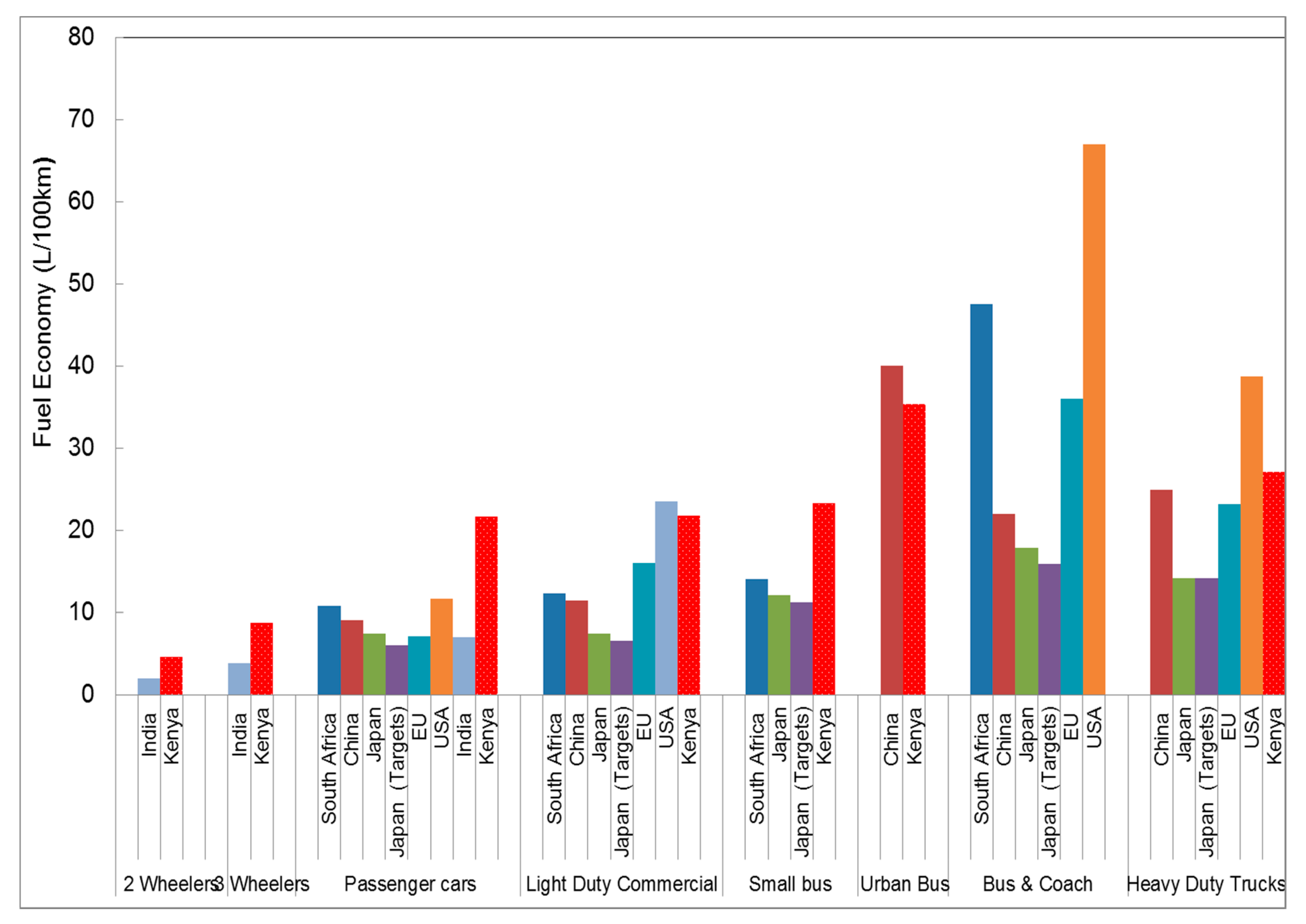
Major vehicle manufacturers (Japan, USA, EU and China) have fuel economy policies [6]. Figure 9 compares the various studies conducted to estimate vehicle fleet fuel economy compared to the current fuel economy values of this study. The Kenyan passenger cars have three times poorer/lower fuel economy compared to the Japanese, EU and Indian fleets and two times lower than the South Africa, Chinese and USA fleets. For the Kenyan light duty commercial vehicles, fuel economy was up to three times poorer compared to the Japanese fleet or targets. Fuel economy of the two-wheelers and three-wheelers of the Kenyan fleet (named bodaboda and tuktuk, respectively) were two times poorer than the corresponding Indian fleet. The matatu 14 seater was determined to be the equivalent to the Japanese small bus (a vehicle designed to carry 11 or more passengers and with GVW up to 3500 kg) and the South African minibus taxi. In this category the Japanese fleet was two times and South Africa fleet was 1.7 times more fuel economic than the matatu 14 seater.

In Kenya, 90% all imported and registered light duty vehicles between 2010–2012 were from Japan and Europe [47]. Japan has very stringent fuel economy standards to meet their 2015 targets [74], yet when the Kenyan fleet is compared to the Japan in-use vehicle fleet in 2004, overall fleet fuel economy was two to three times worse. The comparison in Figure 9 is made on the assumption that other studies have similar or smaller confidence intervals. The confidence interval for the Kenyan study (see Figure 4), ranges from 7–54% with an average of 24%.

The passenger car fuel economy for USA includes light duty trucks [76], while for other countries light duty trucks were a separate category. This may contribute to the seemingly poor fleet fuel economy for passenger cars in the USA, even when the technology and fuels meet the latest equivalent current European and Japanese standards.

The light duty commercial fleet in-use in Nairobi was typically AskforTransport vans and trucks, an informal van and truck hire within the city and in residential areas. This category had the second highest age, as “retired” older vehicles are not scrapped but are repurposed. The fuel economy of this category is better than USA fuel economy for the same category, but USA fleet for this category is heavier (weight of this category in USA includes trucks up to 3800 kg, whilst the other fleets are less than 3500 kg) and bigger engines [6,76].

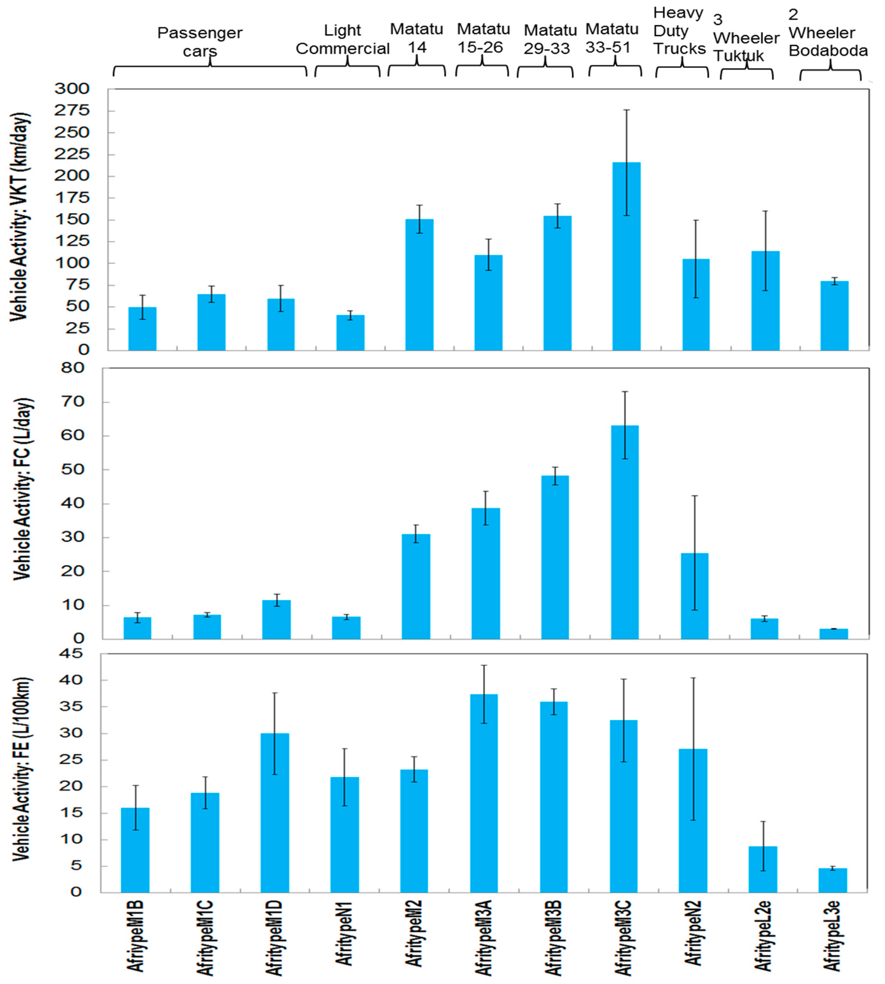
Bodabodas and tuktuks are mainly imported from Asia: India, Indonesia, Thailand, and China, as they are cheaper compared to European imports [30,33]. Motorcycles are used as public transport in India and Vietnam as they are in Kenya, but they have twice the average mileage compared to Kenya, 79.7 ± 4.3 km/day [24,77]. In Asian cities they have a lower daily mileage because they represent a larger share of the urban vehicle fleet, the reason being that motorcycles are often used in Asian cities to avoid congestion, for instance motorcycles represent 90% of the vehicle fleet in Hanoi [77]. Kenyan motorcycles were in this study (see Figure 3) found to be mainly 150 cc engine and 4-stroke engine compared to motorcycles in West Africa that are 50 cc engines and two stroke [33]. Given the trend in increasing numbers of motorcycles in SSA [30,33], the average daily mileage for motorcycles may also decrease. The study also highlighted high intensity vehicle usage, indicated by an average vehicle mileage, VKT, for other vehicle types such as passenger cars (61.04 ± 7.18 km/day), and matatu 151.55 ± 10.42 km/day.

South Africa has a strong domestic vehicle manufacturing industry and restricts imports of second-hand cars [78] and is therefore unlike Kenya where 99% of vehicles are second-hand [47]. Their vehicles perform better than Kenya’s, though reliable minibus taxi data (equivalent to matatu) is often not available. Kenyan matatu 14 seaters are old (16.9 ± 0.2 years) and are originally 9 seater vans converted into 14 seater; overloading and old age is a large component of the fleet; this likely accounts for the poorer fuel economy compared to South Africa. The bigger matatus, equivalent to urban buses, are relatively new and have a better fuel economy comparable to the Chinese fleet. However with expected vehicle technology deterioration [79] further aggravated by poor road conditions, low fuel quality and lack of inspection and maintenance (I/M) programmes this advantage in fuel economy may not be maintained.

The age of the vehicle is normally an indicator of the emission control technology and hence emissions from the vehicle [24,80]. This may hold true for countries that enforce emission compliance checks when importing vehicles and have regular I/M programs [19]. Imported vehicles with emissions control technology often have these removed or they malfunction without an enforceable I/M program [19]. The vehicle fleet average age for four wheelers is often high in Kenya: passenger cars 11.1 ± 0.57 years, matatu 8.80 ± 1.24 years. However, age may not to be a good indicator for emission technology on light duty vehicles in Kenya as a previous study [37] has shown. This is because in Lents et al. [37] the vehicles had the required technology but the fuel quality (unleaded petrol) required may not meet standards for emission reduction devices (catalytic converters) to function. 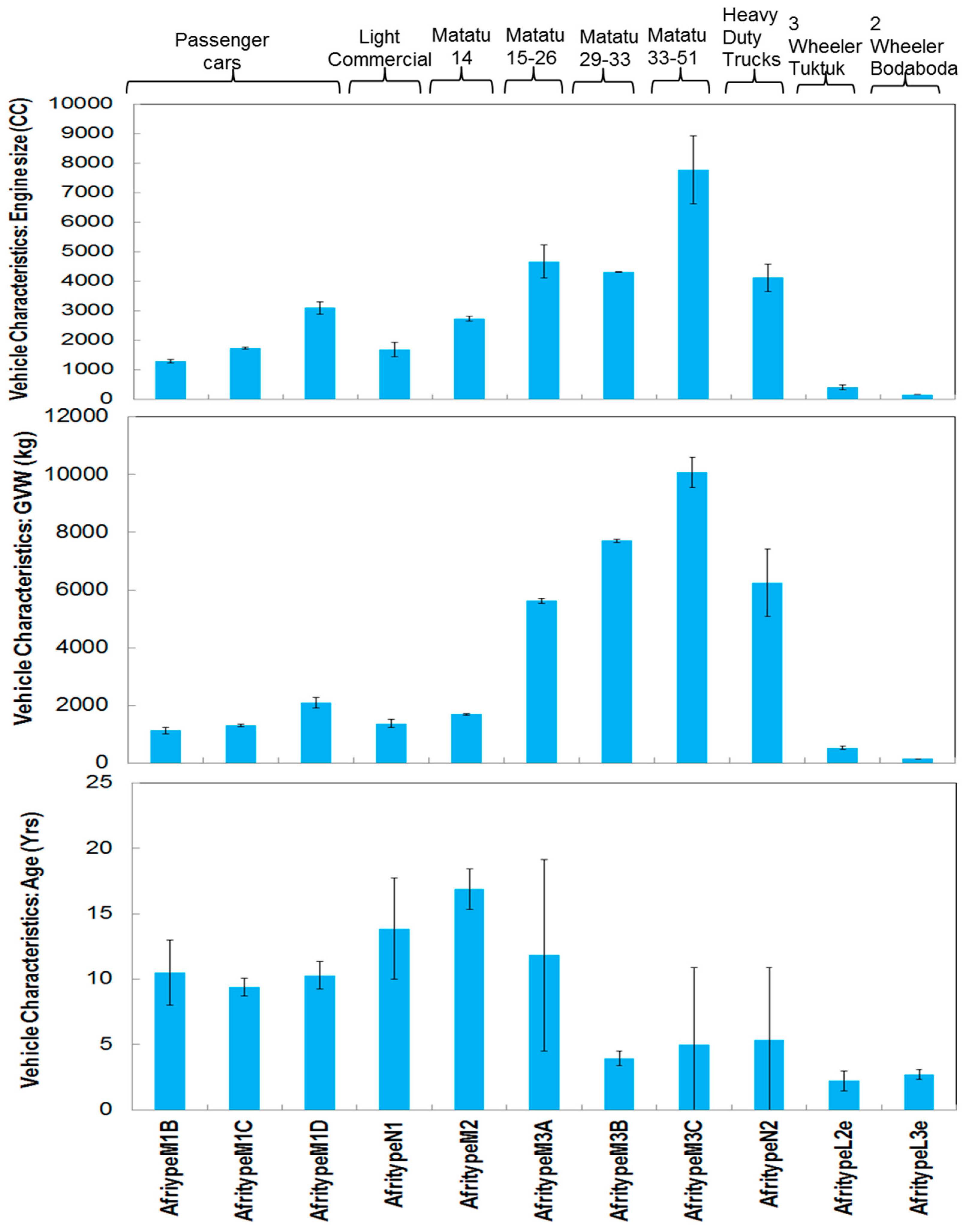Age is also not a good indicator for the technology of emission reduction on HDVs as the original equipment manufacturers (OEMs) are not responsible for the final vehicle configuration other than the powertrain, chassis and cab [81]. This is supported by the findings of this study of a significant variance in the age of HDV (75%), shown in Figure 3: AfritypeM3C and AfritypeN2 differ by 118% and 105% respectively. In Kenya most HDV, such as trucks, are imported as engine chassis and cab and built in the country for various uses: matatus, buses and heavy commercial trucks. However, the sample size for the HDVs for this study was limited, this is because HDVs (trucks and lorries) have limited geographical areas of circulation in Nairobi. Thus, the HDV variance should be viewed cautiously until further studies are conducted with a bigger sample size.

Comparing FE values from different parts of the world is rather uncertain. The studies from which data were compared in Figure 9, had both diesel and petrol vehicles of similar capacity, mass and power specifications. However, identical average properties were not possible for some countries (for example the USA) due to different categories for vehicle weight and engine size. Even when vehicles had identical properties to fleets in other parts of the world, their utility, especially those of the informal sector, were different. To overcome this challenge, developing country fleets (India, South Africa and Thailand) were sought for comparison as their fleets included an informal sector and had similarity in utility. But the informal transport sector in SSA is usually poorly organized and the industry is often deregulated unlike Asia [24,30,33]. The methods to measure FE also differed; real-world exhaust measurement were sought as these were deemed to be most accurate [74,76,82,83] but few such studies are undertaken, thus other in-use vehicle studies were also included [24,29,75]. The year the study was undertaken may also have contributed to the uncertainty as that may change the technology the vehicles may have and the fuel quality. To reduce this effect, the comparator studies were limited to years between 2010–2015. Furthermore, fuel consumption becomes extremely high under traffic congestion [17,84] which is a severe and worsening reality in Nairobi, as in most developing cities [50,85,86,87,88]. Therefore, traffic congestion ought to be factored into FE studies although often, this is not the case [16]. However even with these limitations, we can conclude vehicle activity and thus fuel economy developed for formal transport sectors does not map the complexity of the informal sector due to different vehicle types and utility of the vehicles

4.2. Imputation

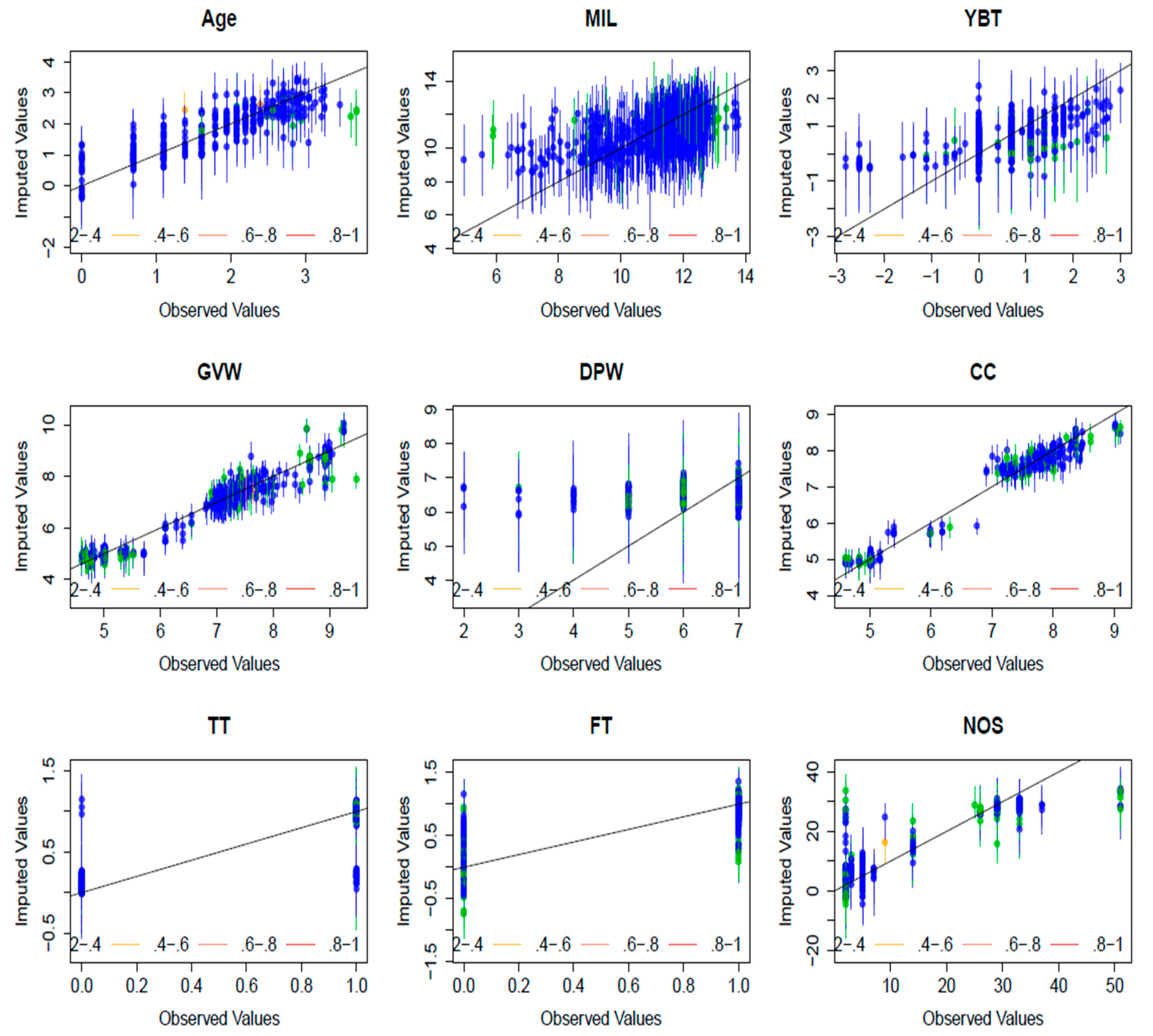
Multiple imputation of incomplete multivariate data was successfully applied to the vehicle fleet data. The diagnostics of the imputation in Figure 6 shows around 90% of the confidence intervals for the variables CC, GVW, Age, MIL, DPW, YBT, TT, FT and NOS contain the y = x line, which means that the true observed value falls within this range, and therefore the imputation was effective in predicting the missing values. The result of the imputation is a bigger data complement than if only those observations for which every variable measured were to be included. The imputation for Engine Size (CC) was a better imputation than Days per Week (DPW). Engine size of the vehicle was verifiable through second-hand vehicle websites and linked to other variables such as GVW, transmission, type of fuel and number of seats. Also, the number of times a vehicle is driven per week (DPW) may be strongly linked to variables not sought after in the questionnaire such as type of job, distance from home or work, fuel price change.

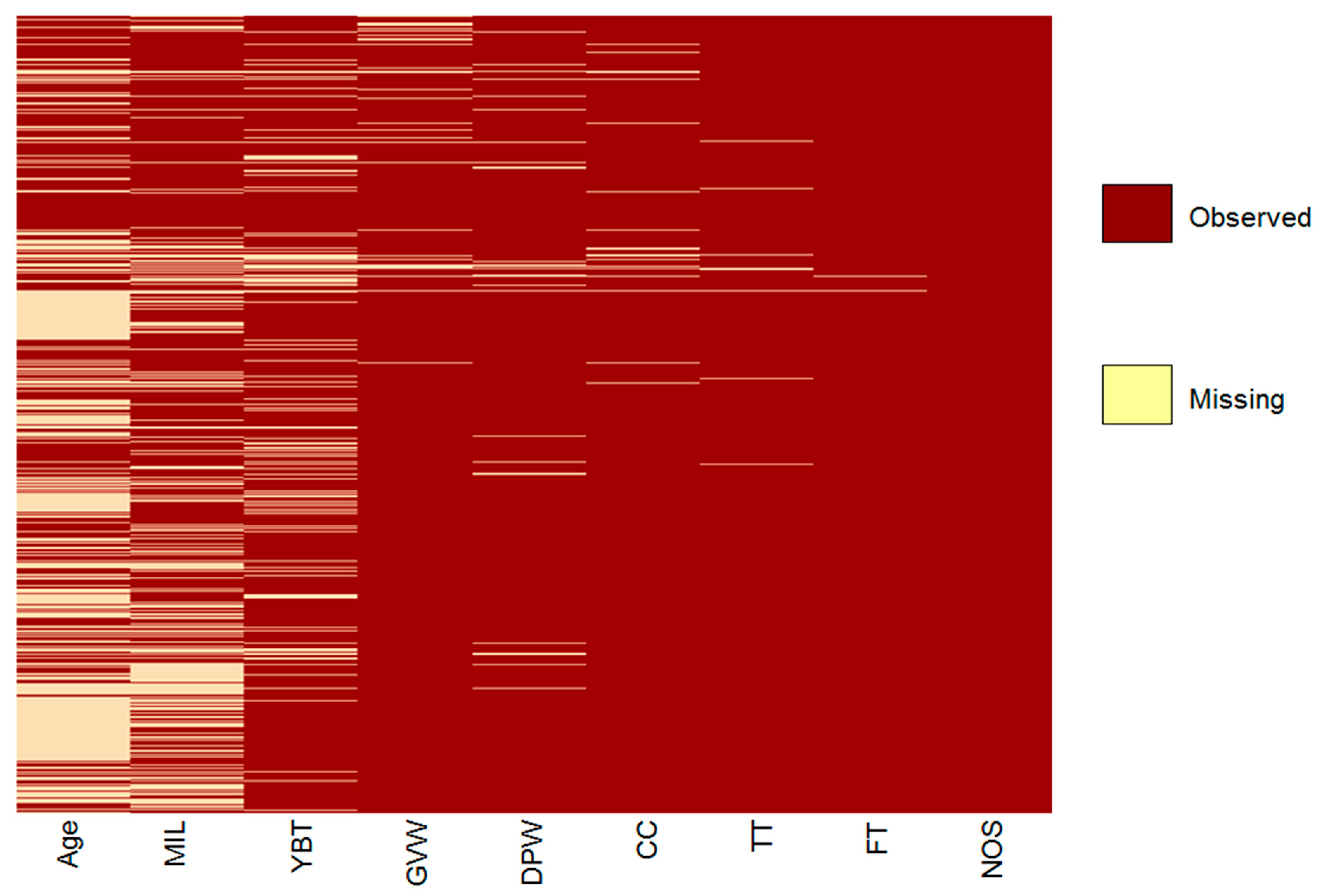
The map of the missing values in Figure 5 shows the variable Age has the most missing values, 46%. This is because during the interviews, if the driver of the vehicle was not the owner, they often did not have the vehicle logbook, thus the age of vehicle, when the vehicle was bought, engine size and weight was not verifiable on site. Secondary data from vehicle sales websites were used to verify and supplement this information where possible. A previous traffic survey in Nairobi was not able to directly ascertain the age of the vehicle and relied on odometer readings as a proxy for the age of vehicles the [36]. This is because at the time vehicle imports were restricted to new vehicles so this proxy worked, in 2015, 99% of vehicles imported are second-hand [47]. MIL, which is the odometer reading, had the second highest missing values, 29%. Drivers of bodabodas, tuktuks, matatus and taxis openly admitted to tampering with the odometers. This finding was supported by a previous study which had very low mileage from a multiple regression methodology to determine average mileage, and concluded that tampering had occurred [36]. Engine size (CC) and GVW were still verifiable via websites thus the missing values were less in the original dataset before the imputation.

4.3. Fuel Economy Model

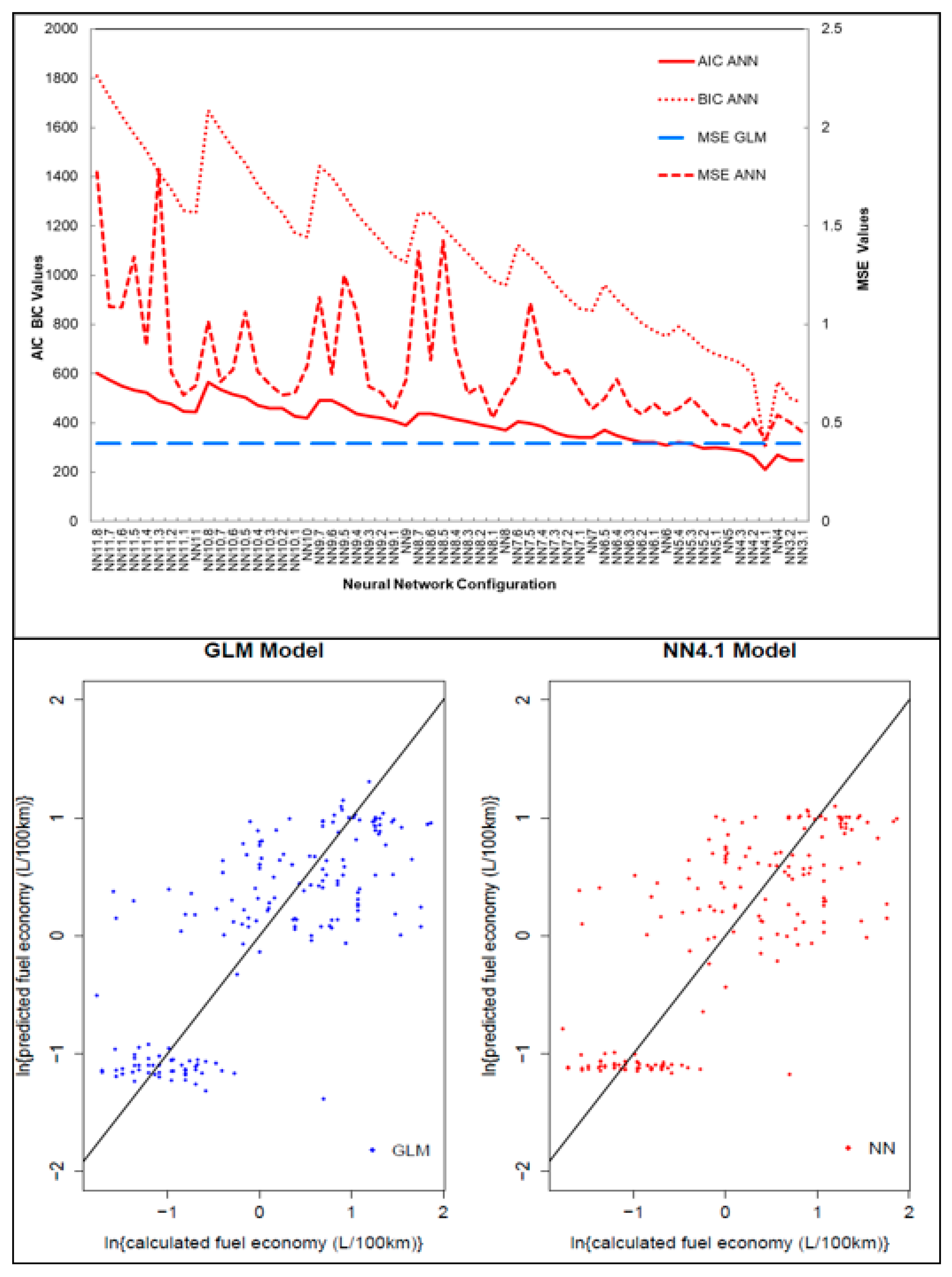
In assessing the comparative statistics in Figure 8, the GLM model consistently performed better than ANN model, engine size was deemed to be most significant in predicting FE. We chose a cross-validation approach to guard our predictor selection approach against over-fitting [39,49,89]. The cross-validation procedure supports our analysis with regards to this goal in three ways. First, the use of information criteria (AIC, BIC) uses indices that provide a numerical summary that takes into account both the fit to the observed data as well as the number of parameters (here layers of the ANN). Unduly complex models were therefore penalised and less likely to end up in our final set of potential models (NN4, NN4.1, NN3.1). Secondly, the use of the MSE in a test sample ensures that if a model is prone to over-fitting the training dataset it will produce worse MSEs in this sample and would again be less likely to be selected. Thirdly, running this analysis as a bootstrap (incl. repeated multiple imputation of missing data adding further robustness) allows us to compare the potential for over/fitting as well as adequate fit in one go. 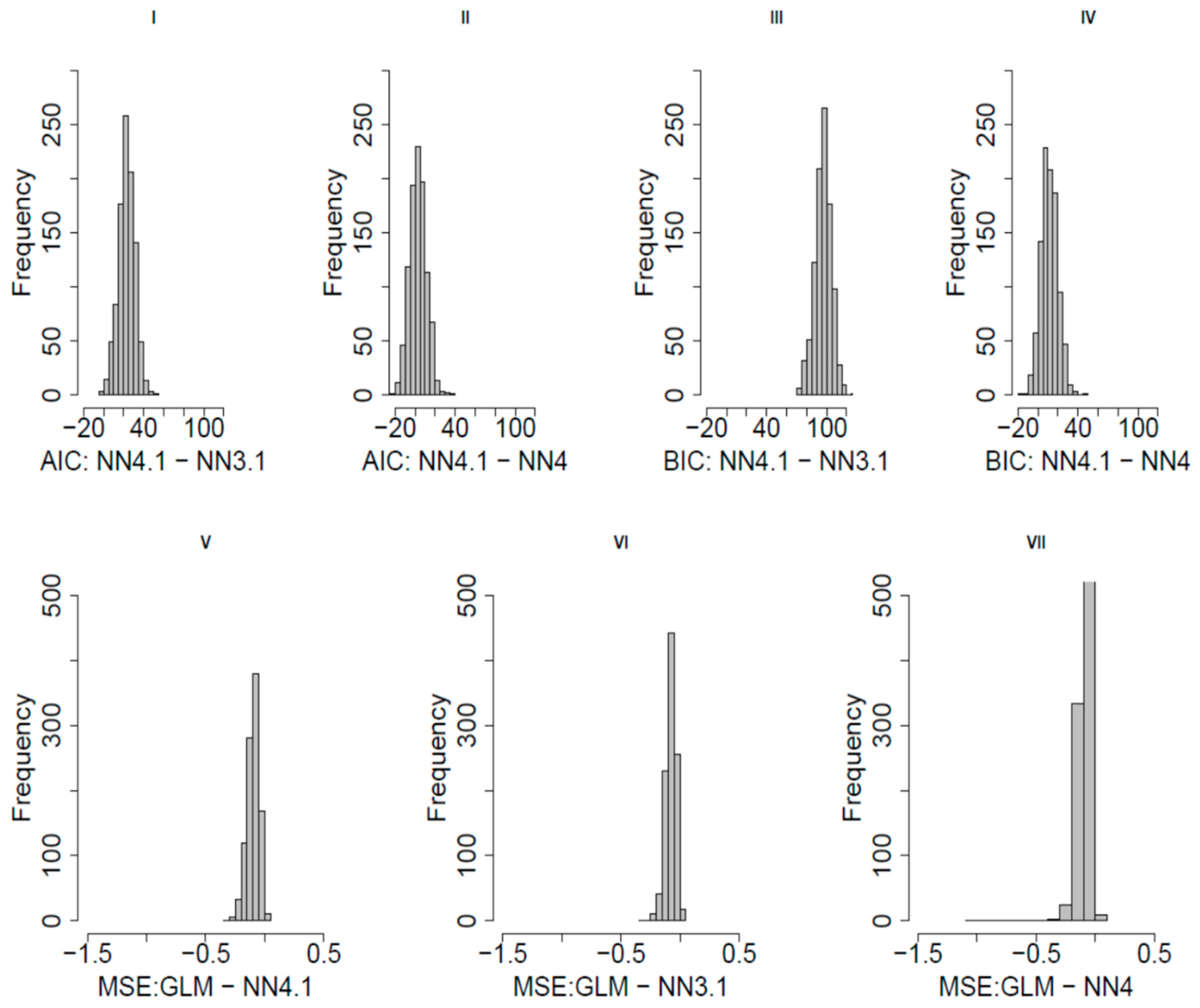Figure 7 shows that the overwhelming majority of the bootstrap runs actually support the fit of simpler neural networks than NN4.1 (NN3.1: AIC in 99.7% and BIC in 100% of runs; NN4: AIC 62.7% BIC 92.2%, respectively) and the MSE supported the GLM consistently (NN4.1 worse than MSE in 99.0%; NN4 in 99.1%; NN3.1 in 98.3% of cross validation runs). The model performance and prediction of the GLM achieved higher accuracy, this finding is contrary to a fuel economy study that compared regression models to ANN, ANN model achieved higher accuracy [39]. This may be because the success of the ANN relies on reliable input and output data to train the algorithm and bigger datasets are better for ANN model precision in prediction for instance Slavin et al. [39] and Alice et al. [49]. Limited and incomplete vehicle fleet data is often a challenge in SSA, so while ANN is a powerful tool in modelling complex relations and systems [39,90,91], due to the smaller dataset it was not the better predictive model when compared to GLM model.

Engine size was deemed to be most significant although three other variables also showed significant relationships with fuel economy: weight of the vehicle (GVW), whether the vehicle was bought in Kenya (UK) and whether it was used overseas (UO), the latter two indicating that these cars consumed more fuel than the newly bought cars. Thus, the study was able to identify aspects of the vehicle fleet character (especially engine size and weight of the vehicle) are key to predicting fuel economy changes, thus providing a focus on those parameters that are vital to obtain while conducting questionnaire surveys in order to derive an accurate estimate of fleet fuel economy.

5. Conclusions

This paper presents a novel methodology that develops a questionnaire and uses the survey data from the questionnaire to develop models to estimate in-use vehicle fleet fuel economy for cities with limited or low-quality data, and that have a large informal transport fleet, such as Nairobi. The vehicle fleets FE in NMR was determined to be 2–3 times worse compared with Japan, Europe, India and China, for example, for the Kenyan passenger vehicles to meet the Japanese fuel economy targets of 5.95 L/100km would require almost a 4-fold improvement in the Kenyan FE. FE models were presented that were based on survey questionnaire data; first data multiple imputations were successfully used to fill in missing data, then modelling performance of different ANN models were compared to a GLM model. The GLM model consistently performed better than the ANN model. Engine size was deemed to be most significant factor in predicting FE.

In cities such as Nairobi that are experiencing a rapid growth in transport emissions, predicting fuel economy changes in response to changes in vehicle characteristics and activity can help inform effective transport policies that rely on the availability of robust data and the application of sound assessment methods. A baseline measure of fuel economy for both the formal and informal vehicle fleet in NMR has now been established for 2015. This identifies the substantial contribution the informal vehicle fleet is currently making to the air pollution and GHG burden. This is particularly important given the trends in this fleet component which suggest a continued increase in size of this informal transport sector with no new regulations. Application of these methods can help identify the rise of informal transport as a particularly polluting component of the transport sector and help target fuel economy improvements in changing vehicle fleets in the future. It also identifies the need to take further action to address informal transport from an air quality management and GHG emission perspective. Furthermore, vehicle activity data presented here would improve Kenya’s NDC formulation for the transport sector. Ultimately, this will aid sustainable road transport policy implementation, which will lead to a reduction in fuel consumption and improvement of FE, leading tor reductions in GHGs emissions and improvements in air quality.

References

1. Ribeiro, K.; Kobayashi, S.; Beuthe, M.; Gasca, J.; Green, D.; Lee, S.D. Contribution of Working Group III to the Fourth Assessment Report of the Intergovernmental Panel on Climate Change. In Climate Change 2007: Mitigation; Metz, B., Davidson, O.R., Bosch, P.R., Dave, R., Meyer, L.A., Eds.; Cambridge University Press: Cambridge, UK; New York, NY, USA, 2007; pp. 324–385. Available online: http://www.ipcc.ch/publications_and_data/ar4/wg3/en/ch5.html (accessed on 7 February 2014).
2. Schipper, L. Automobile use, fuel economy and CO2 emissions in industrialized countries: Encouraging trends through 2008? Transp. Policy 2011, 18, 358–372. [Google Scholar] [CrossRef]
3. IEA. International Comparison of Light-Duty Vehicle Fuel Economy and Related Characteristics. 2011. Available online: http://www.globalfueleconomy.org/Documents/Publications/wp5_iea_fuel_Economy_report.pdf (accessed on 16 June 2014).
4. IEA. Technology Roadmap Fuel Economy of Road Vehicles. 2012. Available online: https://www.iea.org/publications/freepublications/publication/technology-roadmap-fuel-economy-of-road-vehicles.html (accessed on 16 June 2014).
5. Bandivadekar, A.; Miller, J.; Kodjak, D.; Muncrief, R.; Yang, Z.; De Jong, R. Fuel Economy State of the World. 2016. Available online: http://www.globalfueleconomy.org/media/203446/gfei-state-of-the-world-report-2016.pdf (accessed on 15 May 2017).
6. Plotkin, S. Fuel Economy Initiatives: A Worldwide Comparison. In Reference Module in Earth Systems and Environmental Sciences; Elsevier: Amsterdam, The Netherlands, 2016. [Google Scholar]
7. Goel, R.; Guttikunda, S.K.; Mohan, D.; Tiwari, G. Benchmarking Vehicle and Passenger Travel Characteristics in Delhi for on-road Emissions Analysis. Travel. Behav. Soc. 2014, 2, 88–101. [Google Scholar] [CrossRef]
8. Goel, R.; Mohan, D.; Guttikunda, S.K.; Tiwari, G. Assessment of Motor Vehicle use Characteristics in Three Indian Cities. Transp. Res. Part D Transp. Environ. 2015, 44, 254–265. [Google Scholar] [CrossRef]
9. Kholod, N.; Evans, M.; Gusev, E.; Yu, S.; Malyshev, V.; Tretyakova, S.; Barinov, A. A methodology for calculating transport emissions in cities with limited traffic data: Case study of diesel particulates and black carbon emissions in Murmansk. Sci. Total Environ. 2016, 547, 305–313. [Google Scholar] [CrossRef]
10. Agyemang-Bonsu, K.W.; Dontwi, I.K.; Tutu-Benefoh, D.; Bentil, D.E.; Boateng, O.G.; Asuobonteng, K.; Agyemang, W. Traffic-data driven modelling of vehicular emissions using COPERT III in Ghana: A case study of Kumasi. Am. J. Sci. Ind. Res. 2010, 134350, 32–40. [Google Scholar]
11. Ommeh, M.; McCormick, D.; Mitullah, W.; Risper, O.; Preston, C. The Politics Behind the Phasing Out of the 14-seater Matatu in Kenya. University Nairobi Digit Repos. 2015, pp. 1–16. Available online: http://erepository.uonbi.ac.ke/handle/11295/85489 (accessed on 15 May 2017).
12. Behrens, R.; McCormick, D.; Orero, R.; Ommeh, M. Improving paratransit service: Lessons from inter-city matatu cooperatives in Kenya. Transp. Policy. 2017, 53, 79–88. [Google Scholar] [CrossRef]
13. Venter, C.; Mohammed, S. Estimating car ownership and transport energy consumption: A disaggregate study in Nelson Mandela Bay. J. South Afr. Inst. Civ. Eng. 2013, 55, 2–10. [Google Scholar]
14. Kumar, A. Understanding the Emerging Role of Motorcycles in African Cities: A Political Economy Perspective; Discussion Paper; Sub-Saharan Africa Transport Policy Program (SSATP): Washington, DC USA, 2011; Volume 13. [Google Scholar]
15. Kumar, A.; Barrett, F. Stuck in Traffic: Urban Transport in Africa. AICD Backgr Pap 2008. Available online: http://siteresources.worldbank.org/EXTAFRSUBSAHTRA/Resources/Stuck-in-Traffic.pdf (accessed on 22 May 2014).
16. Cervero, R.; Golub, A. Informal transport: A global perspective. Transp. Policy 2007, 14, 445–457. [Google Scholar] [CrossRef]
17. Assamoi, E.-M.; Liousse, C. A new inventory for two-wheel vehicle emissions in West Africa for 2002. Atmos. Environ. 2010, 44, 3985–3996. [Google Scholar] [CrossRef]
18. Doumbia, M.; Toure, N.E.; Silue, S.; Yoboue, V.; Diedhiou, A.; Hauhouot, C.A. Emissions from the Road Traffic of West Africa’s Cities: Assessment of Vehicle Fleet and Fuel Consumption. Energies 2018, 11, 2300. [Google Scholar] [CrossRef]
19. Lents, J.; Davis, N.; Nikkila, N.; Osses, M.; Martinez, H.; Ehsani, S. Measurement of In-Use Passenger Vehicle Emissions in Three Urban Areas of Developing Nations. 2005. Available online: http://www.issrc.org/ive/downloads/reports/VER3Cities.pdf (accessed on 24 November 2014).
20. UC Riverside. Nairobi, Kenya Vehicle Activity Study. 2002. Available online: www.issrc.org/ive/downloads/reports/NairobiKenya.pdf (accessed on 18 July 2014).
21. Lents, J.; Davis, N.; Osses, M.; Nikkila, R.; Barth, M. Comparison of on-road vehicle profiles collected in seven cities worldwide. Transp. Air 2004, 1–24. Available online: http://issrc.org/ive/downloads/presentations/IVE_TAP_2004.pdf (accessed on 16 July 2014).
22. Plotkin, S. Fuel Economy Initiatives: International Comparisons. In Encyclopedia of Energy; Cleveland, C., Ed.; Elsevier: Amsterdam, The Netherlands, 2004; Volume 2, pp. 791–806. [Google Scholar]
23. Tietge, U.; Mock, P.; Franco, V.; Zacharof, N. From laboratory to road: Modeling the divergence between official and real-world fuel consumption and CO2 emission values in the German passenger car market for the years 2001–2014. Energy Policy 2017, 103, 212–222. [Google Scholar] [CrossRef]
24. Hao, H.; Wang, S.; Liu, Z.; Zhao, F. The impact of stepped fuel economy targets on automaker’s light-weighting strategy: The China case. Energy 2016, 94, 755–765. [Google Scholar] [CrossRef]
25. Huo, H.; He, K.; Wang, M.; Yao, Z. Vehicle technologies, fuel-economy policies, and fuel-consumption rates of Chinese vehicles. Energy Policy 2012, 43, 30–36. [Google Scholar] [CrossRef]
26. Haq, G.; Weiss, M. CO2 labelling of passenger cars in Europe: Status, challenges, and future prospects. Energy Policy 2016, 95, 324–335. [Google Scholar] [CrossRef]
27. Slavin, D.; Abou-Nasr, A.; Filev, D.; Kolmanovsky, I. Empirical Modeling of Vehicle Fuel Economy Based on Historical Data. IEEE, 2013; p. 313. Available online: http://ieeexplore.ieee.org/stamp/stamp.jsp?arnumber=6707111 (accessed on 31 March 2016).
28. Ntziachristos, L.; Mellios, G.; Tsokolis, D.; Keller, M.; Hausberger, S.; Ligterink, N.E.; Dilara, P. In-use vs. type-approval fuel consumption of current passenger cars in Europe. Energy Policy 2014, 67, 403–411. [Google Scholar] [CrossRef]
29. TÜV Nord. ICCT Fuel Economy Data Collection Pilot Study. 2013. Available online: http://www.theicct.org/sites/default/files/TNM_ICCT_FE_Data_Collection_Pilot_Study_ProjectReport_Final2.pdf (accessed on 6 June 2016).
30. Cameron, L.; Wurtenberger, L.; Stiebert, S. Kenya’s Climate Change Action Plan: Mitigation Chapter 7: Transportation. 2012. Available online: http://www.kccap.info/index.php?option=com_phocadownload&view=category&id=36 (accessed on 14 June 2016).
31. ERC. Report on Global Fuel Economy Initiative Study in Kenya (GFEI). 2015. Available online: http://www.erc.go.ke/index.php?option=com_content&view=article&id=224&Itemid=721 (accessed on 23 August 2015).
32. Posada, A.F.; German, J. Measuring In-Use Fuel Economy in Europe and the US: Summary of Pilot Studies. 2013. Available online: http://www.theicct.org/measuring-in-use-fuel-economy-summary-pilot-studies (accessed on 23 August 2015).
33. Weiss, M.; Bonnel, P.; Hummel, R.; Provenza, A.; Manfredi, U. On-road emissions of light-duty vehicles in Europe. Environ. Sci. Technol. 2011, 45, 8575–8581. [Google Scholar] [CrossRef] [PubMed]
34. Tiege, U.; Zacharof, N.; Mock, P.; Franco, V.; German, J.; Bandivadekar, A. From Laboratory to Road. 2015. Available online: http://www.theicct.org/sites/default/files/publications/ICCT_LaboratoryToRoad_2015_Report_English.pdf (accessed on 29 August 2016).
35. Pandey, A.; Venkataraman, C. Estimating emissions from the Indian transport sector with on-road fleet composition and traffic volume. Atmos Environ. 2014, 98, 123–133. [Google Scholar] [CrossRef]
36. Zhang, S.; Wu, Y.; Liu, H.; Huang, R.; Un, P.; Zhou, Y.; Fu, L.; Hao, J. Real-world fuel consumption and CO2 (carbon dioxide) emissions by driving conditions for light-duty passenger vehicles in China. Energy 2014, 69, 247–257. [Google Scholar] [CrossRef]
37. Hu, J.; Wu, Y.; Wang, Z.; Li, Z.; Zhou, Y.; Wang, H. Real-world fuel efficiency and exhaust emissions of light-duty diesel vehicles and their correlation with road conditions. J. Environ. Sci. 2012, 24, 865–874. [Google Scholar] [CrossRef]
38. Smit, R.; Brown, A.L.; Chan, Y.C. Do air pollution emissions and fuel consumption models for roadways include the effects of congestion in the roadway traffic flow? Environ. Model Softw. 2008, 23, 1262–1270. [Google Scholar] [CrossRef]
39. Zhang, S.; Wu, Y.; Liu, H.; Ruikun, H.; Yang, L.; Li, Z. Real-world fuel consumption and CO2 emissions of urban public buses in Beijing. Appl. Energy 2014, 113, 1645–1655. [Google Scholar] [CrossRef]
40. Boulter, P.G.; Barlow, T.J.; Mccrae, I.S. Exhaust Mission Factors for Road Vehicles in the United Kingdom. 2009. Available online: https://www.gov.uk/government/uploads/system/uploads/attachment_data/file/4249/report-3.pdf (accessed on 24 March 2018).
41. Pillot, D.; Legrand-tiger, A.; Thirapounho, E.; Tassel, P.; Perret, P. Impacts of Inadequate Engine Maintenance on Diesel Exhaust Emissions. In Proceedings of the Transport Research Arena, Paris, France, 14 April 2014. [Google Scholar]
42. Schwela, D. Review of Urban Air Quality in Sub-Saharan Africa Region-Air Quality Profile of SSA Countries. 2012. Available online: http://www-wds.worldbank.org/external/default/WDSContentServer/WDSP/IB/2012/04/02/000386194_20120402015455/Rendered/PDF/677940WP0P07690020120Box367897B0ACS.pdf (accessed on 31 January 2014).
43. United Nations. United Nations Framework Convention on Climate Change; Fccc/Informal/84; United Nations: New York, NY, USA, 1992; pp. 270–277. [Google Scholar] [CrossRef]
44. Cappiello, A.; Chabini, I.; Nam, E.; Lue, A.; Zeid, A. A Statistical Model of Vehicle Emissions and Fuel Consumption. IEEE, 2002; pp. 801–809. Available online: http://ieeexplore.ieee.org/xpls/abs_all.jsp?arnumber=1041322 (accessed on 02 June 2016).
45. Oh, Y.; Park, J.; Lee, J.; Eom, M.D.; Park, S. Modeling effects of vehicle specifications on fuel economy based on engine fuel consumption map and vehicle dynamics. Transp. Res. Part D Transp. Environ. 2014, 32, 287–302. [Google Scholar] [CrossRef]
46. Ibarra-espinosa, S.; Ynoue, R.; Sullivan, S.O.; Pebesma, E.; Andrade, M.D.F.; Osses, M. VEIN v0.2.2: An R package for bottom-up Vehicular Emissions Inventories. Geosci. Model Dev. Dis. 2018, 11, 2209–2229. [Google Scholar] [CrossRef]
47. Goyns, P.H. Modelling Real-World Driving, Fuel Consumption and Emissions of Passenger Vehicles: A Case Study in Johannesburg; University of Johannesburg: Johannesburg, South Africa, 2008. [Google Scholar]
48. Honaker, J.; King, G.; Blackwell, M. AMELIA II: A Program for Missing Data. J. Stat. Softw. 2011, 45, 1–54. [Google Scholar] [CrossRef]
49. Alice, M. Fitting a Neural Network in R Neuralnet Package. Datascienceplus. 2015. Available online: http://datascienceplus.com/fitting-neural-network-in-r/ (accessed on 13 June 2016).
50. UN-HABITAT. The State of African Cities 2014: Re-Imagining Sustainable Urban Transitions; UN-HABITAT: Nairobi, Kenya, 2014; 278p. [Google Scholar]
51. KNBS. Kenya National Bureau of Statistics Kenya Facts and Figures. 2014. Available online: http://www.knbs.or.ke/index.php?option=com_phocadownload&view=category&id=20&Itemid=1107 (accessed on 23 August 2015).
52. JICA. The Study on Master Plan for Urban Transport in the Nairobi Metropolitan Area in The Republic of Kenya; JICA: Nairobi, Kenya, 2006.
53. JICA. The Project on Integrated Urban Development Master Plan for the City of Nairobi in the Republic of Kenya Final Report; JICA: Nairobi, Kenya, 2014.
54. Lansley, G. Regional Studies, Regional Science Cars and socio-economics: Understanding neighbourhood variations in car characteristics from administrative data Cars and socio-economics: Understanding administrative data. Reg. Stud. Reg. Sci. 2016, 3, 264–286. [Google Scholar] [CrossRef]
55. GRASS Development Team. Geographic Resources Analysis Support System (GRASS) Software. Open Source Geospatial Foundation. 2015. Available online: https://grass.osgeo.org/home/about-us/ (accessed on 20 July 2016).
56. Gachanja, J.N. Evaluating the Impact of Road Traffic Congestion Mitigation Measures in Nairobi Metropolitan Region; Infrastructure and Ecopnomic Services Division: Nairobi, Kenya, 2012. [Google Scholar]
57. Van Dessel, G. How to Determine Population and Survey Sample Size? 2013. Available online: https://www.checkmarket.com/2013/02/how-to-estimate-your-population-and-survey-sample-size/ (accessed on 27 August 2014).
58. Fincham, J.E. Response rates and responsiveness for surveys, standards, and the Journal. Am. J. Pharm. Educ. 2008, 72, 43. [Google Scholar] [CrossRef]
59. Be Foward Co. Japanese Used Cars. 2017. Available online: http://www.beforward.jp/ (accessed on 24 April 2017).
60. Cheki Inc. New and Used Cars for Sale in Kenya. 2017. Available online: https://www.cheki.co.ke/ (accessed on 24 April 2017).
61. Japan Car Direct. The Toyota Hiace Van for East Africa-Japan Car Direct. 2015. Available online: http://www.japancardirect.com/buy-second-hand-cars-from-japan-domestic-market-from-japan-car-direct/the-toyota-hiace-van-for-east-africa (accessed on 17 June 2015).
62. PigiaMe. Cars for Sale in Kenya. 2017. Available online: https://www.pigiame.co.ke/cars (accessed on 24 April 2017).
63. Isuzu Kenya. Isuzu-Kenya Bus Specifications. 2014. Available online: http://www.isuzutrucks.co.ke/33-seater-bus#overview (accessed on 11 December 2014).
64. Toyota. Toyota Global Website. 2017. Available online: http://www.toyota-global.com/ (accessed on 24 April 2017).
65. Toyota Kenya. Toyota Hiace Specifications. 2014. Available online: https://www.toyotakenya.com/products.php?products_id=49 (accessed on 11 December 2014).
66. Toyota Kenya. Toyota Kenya Ltd. 2017. Available online: https://www.toyotakenya.com/ (accessed on 24 April 2017).
67. Nissan Kenya. Nissan. 2017. Available online: http://www.nissankenya.com/ (accessed on 24 April 2017).
68. Kouridis, C.; Samaras, C.; Hassel, D.; Mellios, G.; Mccrae, I.; Zierock, K. Road Transport. In EMEP/EEA Air Pollutant Emission Inventory Guidebook-2016; European Economic Area: Brussels, Belgium, 2016. [Google Scholar]
69. R Core Team. R: A Language and Environment for Statistical Computing; R Foundation for Statistical Computing: Vienna, Austria, 2016. [Google Scholar]
70. ERC. Fuel Prices at the Pump. 2015. Available online: http://www.erc.go.ke/index.php?option=com_content&view=article&id=162&Itemid=666 (accessed on 3 August 2015).
71. Total Motorcycle. Total Motorcyle Fuel Economy Guide in MPG and L/100km; Total Motorcycle: Houston, TX, USA, 2017; pp. 1–2. [Google Scholar]
72. NHTSA. Summary of Fuel Economy Perfomance; U.S. Department of Transportation: Washington, DC, USA, 2014.
73. Nagendra, S.M.S.; Khare, M. Modelling urban air quality using artificial neural network. Clean Technol. Environ. Policy 2005, 7, 116–126. [Google Scholar] [CrossRef]
74. JAMA. 2016 Report on Environmental Protection Efforts Promoting Sustainability in Road Transport in Japan; Japan Automobile Manufacturers Association, Inc.: Tokyo, Japan, 2016. [Google Scholar]
75. Law, K.; Jackson, M.; Chan, M. European Union Greenhouse Gas Reduction Potential for Heavy-Duty Vehicles. 2011. Available online: http://ec.europa.eu/clima/policies/transport/vehicles/heavy/docs/icct_ghg_reduction_potential_en.pdf (accessed on 3 September 2015).
76. EPA. Light-Duty Automotive Technology, Carbon Dioxide Emissions, and Fuel Economy Trends: 1975 Through 2014. 2014. Available online: https://catalog.data.gov/dataset/light-duty-automotive-technology-carbon-dioxide-emissions-and-fuel-economy-trends-data-5ff55 (accessed on 10 June 2015).
77. Oanh, N.T.; Thuy Phuong, M.T.; Permadi, D.A. Analysis of motorcycle fleet in Hanoi for estimation of air pollution emission and climate mitigation co-benefit of technology implementation. Atmos. Environ. 2012, 59, 438–448. [Google Scholar] [CrossRef]
78. UNEP. Status of Fuel Quality and Vehicle Emission Standards: Sub Saharan Africa. 2015. Available online: http://www.unep.org/Transport/new/PCFV/pdf/Maps_Matrices/Africa/matrix/SSAFuels_Veh_matrix_June2015.pdf (accessed on 15 September 2015).
79. Chiang, H.-L.; Tsai, J.-H.; Yao, Y.-C.; Ho, W.-Y. Deterioration of gasoline vehicle emissions and effectiveness of tune-up for high-polluted vehicles. Transp. Res. Part D Transp. Environ. 2008, 13, 47–53. [Google Scholar] [CrossRef]
80. Zachariadis, T.; Ntziachristos, L.; Samaras, Z. The effect of age and technological change on motor vehicle emissions. Transp. Res. Part D Transp. Environ. 2001, 6, 221–227. [Google Scholar] [CrossRef]
81. Hill, N.; Finnegan, S.; Norris, J.; Brannigan, C.; Wyann, D.; Baker, H. Reduction and Testing of Greenhouse Gas (GHG) Emissions from Heavy Duty Vehicles—Lot 1: Strategy. AEA/Ricardo, 2011. Available online: https://circabc.europa.eu/sd/a/bb7ac696-7767-4a49-ab10-0f05f1606599/2010%2520FQM%2520report+&cd=3&hl=en&ct=clnk&gl=hk (accessed on 22 September 2015).
82. Huo, H.; Yao, Z.; He, K.; Yu, X. Fuel consumption rates of passenger cars in China: Labels versus real-world. Energy Policy 2011, 39, 7130–7135. [Google Scholar] [CrossRef]
83. Franco, V.; Kousoulidou, M.; Muntean, M.; Ntziachristos, L.; Hausberger, S.; Dilara, P. Road vehicle emission factors development: A review. Atmos. Environ. 2013, 70, 84–97. [Google Scholar] [CrossRef]
84. Wang, H.; Fu, L.; Zhou, Y.; Li, H. Modelling of the fuel consumption for passenger cars regarding driving characteristics. Transp. Res. Part D Transp. Environ. 2008, 13, 479–482. [Google Scholar] [CrossRef]
85. Kinney, P.L.; Gichuru, M.G.; Volavka-Close, N.; Ngo, N.; Ndiba, P.K.; Law, A. Traffic Impacts on PM (2.5) Air Quality in Nairobi, Kenya. Environ. Sci. Policy 2011, 14, 369–378. Available online: http://www.sciencedirect.com/science/article/pii/S1462901111000189 (accessed on 10 February 2014). [CrossRef]
86. Salon, D.; Aligula, E.M. Urban travel in Nairobi, Kenya: Analysis, insights, and opportunities. J. Transp. Geogr. 2012, 22, 65–76. [Google Scholar] [CrossRef]
87. Gyimesi, K.; Vincent, C.; Lamba, N. Frustration Rising: IBM 2011 Commuter Pain Survey. 2011. Available online: http://www.ibm.com/smarterplanet/us/en/traffic_congestion/ideas/index.html (accessed on 26 February 2014).
88. Petkova, E.P.; Jack, D.W.; Volavka-Close, N.H.; Kinney, P.L. Particulate matter pollution in African cities. Air Qual. Atmos. Heal. 2013, 6, 603–614. [Google Scholar] [CrossRef]
89. Arlot, S.; Celisse, A. A survey of cross-validation procedures for model selection. Stat Surv. 2010, 4, 40–79. [Google Scholar] [CrossRef]
90. Goh, A.T.C. Back-propagation neural networks for modeling complex systems. Artif. Intell. Eng. 1995, 9, 143–151. [Google Scholar] [CrossRef]
91. Molaie, M.; Falahian, R.; Gharibzadeh, S.; Jafari, S.; Sprott, J.C.; Mattei, T.A. Artificial neural networks: powerful tools for modeling chaotic behavior in the nervous system. Comput. Nuerosci. 2014, 8, 40. [Google Scholar] [CrossRef] [PubMed]
92. Horton, N.J.; Lipsitz, S.R. Multiple imputation in practice: Comparison of software packages for regression models with missing variables. Am. Stat. 2001, 55, 244–254. [Google Scholar] [CrossRef]
93. Kenward, M.G.; Carpenter, J. Multiple imputation: current perspectives. Stat. Methods Med. Res. 2007, 16, 199–218. [Google Scholar] [CrossRef] [PubMed]
94. Azur, M.J.; Stuart, E.A.; Frangakis, C.; Leaf, P.J. Multiple imputation by chained equations: What is it and how does it work? Int. J. Methods Psychiatr. Res. 2011, 20, 40–49. [Google Scholar] [CrossRef] [PubMed]
95. Burton, A.; Billingham, L.J.; Bryan, S. Cost-effectiveness in clinical trials: using multiple imputation to deal with incomplete cost data. Clin. Trials. 2007, 4, 154–161. [Google Scholar] [CrossRef] [PubMed]
96. Biering, K.; Hjollund, N.H.; Frydenberg, M. Using multiple imputation to deal with missing data and attrition in longitudinal studies with repeated measures of patient-reported outcomes. Clin. Epidemiol. 2015, 7, 91–106. [Google Scholar] [CrossRef] [PubMed]
97. Fritsch, S.; Guenther, F.; Suling, M.; Mueller, M.S. Training of Neural Networks. Available online: https://cran.r-project.org/web/packages/neuralnet/neuralnet.pdf (accessed on 7 February 2019).
Figure 1. The data combinations required to develop the NMR vehicle fleet dataset and estimate fuel economy using the three different modelling approaches: calculated fuel economy, GLM and ANN.
Energies 12 01177 g001
Figure 2. A map of the 15 field sites where the questionnaire survey interviews were conducted in the NMR. The map was created using GRASS software [55].
Energies 12 01177 g002
Figure 3. Vehicle characteristics from questionnaire data, mean with 95% confidence interval for vehicle age, engine size, and weight.
Energies 12 01177 g003
Figure 4. Vehicle activity from questionnaire data, mean and 95% confidence interval about the mean of the vehicle kilometres travelled (VKT), fuel consumption (FC) and Fuel Economy (FE′) for Kenyan classes.
Energies 12 01177 g004
Figure 5. A map of missing values. The variables in columns correspond with those from Equation (3) as follows: Age (age of vehicle as proxy for technology), MIL (mileage on the car from cumulated odometer reading), YBT (vehicle turnover from years since vehicle bought by current owner), GVW (gross value weight), DPW (days per week vehicle used), CC (engine size), TT (transmission type), FT (fuel type), NOS (number of seats on vehicle). The y-axis presents the count of the different variables.
Energies 12 01177 g005
Figure 6. Diagnostic graph of observed variables plotted against the imputed values.
Energies 12 01177 g006
Figure 7. A comparison of GLM and various configurations ANN model and then the best NN model (two layers, four and one neuron) is compared to the GLM model. NNij denotes the network configuration of the neural network with i, the number of nodes in the first layer and j the number of nodes in the second layer. All the values in these plots are log-normal transformed. The plot on the bottom half of the figure, x-axis represents calculated fuel economy (FE′) and the y-axis is predicted fuel economy (FE″).
Energies 12 01177 g007
Figure 8. Plot of the comparative statistics of the bootstrap. AIC, BIC, MSE of the three top ANN models (NN4.1, NN3.1, NN4) and the GLM model. I, II, III, IV comprises of AIC and BIC comparisons of ANN and V, VI, VII comprises of MSE comparisons of GLM and ANN.
Energies 12 01177 g008
Figure 9. Fuel economies for different countries from various sources: India [24], Kenya (current study), South Africa [29], China [44], Japan [74], EU [14,75], USA [75,76].
Energies 12 01177 g009