Article

Impedance Estimation with an Enhanced Particle Swarm Optimization for Low-Voltage Distribution Networks

1
School of Electrical Engineering, Kyungpook National University, Daegu 41566, Korea
2
School of Mechanical Engineering, Keimyung University, Daegu 702701, Korea
3
Department of Creative IT Engineering, Pohang University of Science and Technology, Pohang 37673, Korea
*
Author to whom correspondence should be addressed.
Energies 2019, 12(6), 1167; https://doi.org/10.3390/en12061167
Submission received: 14 February 2019 / Revised: 18 March 2019 / Accepted: 21 March 2019 / Published: 26 March 2019
(This article belongs to the Special Issue Machine Learning and Optimization with Applications of Power System)

Abstract

:
Many researchers in recent years have studied voltage deviation issues in distribution networks. Characterizing the impedance between consuming nodes in a network is the key to controlling the network voltage. Existing impedance estimation methods are faced with three challenges: time synchronized measurement, a generalization of the network model, and convergence of the optimization for objective functions. This paper extends an existing impedance estimation algorithm by introducing an enhanced particle swarm optimization (PSO). To overcome this method’s local optimum problem, we propose adaptive inertia weights. Also, our proposed method is based on a new general model for a low voltage distribution network with non-synchronized measurements. In the case study, the improved impedance estimation algorithm realizes better accuracy than the existing method.

1. Introduction

With the increasing penetration of residential and commercial photovoltaic systems (PVs) in distribution networks, PV power generation can cause reverse power flow through the distribution system. Significant reverse power flow may cause operational issues such as overvoltage on the feeders, increased short circuit current, or excessive operation of control equipment to keep the voltage and current within required bounds [1]. PVs are recognized as major contributors to network voltage deviation, especially in low voltage distribution networks. This characteristic of PVs is one of the greatest barriers to increasing the general penetration of PVs in low-voltage distribution networks [2] and is even more prominent in rural networks [3].
Various existing studies have addressed the voltage deviation problem caused by PVs. Case studies in [1] were performed pertaining to voltage stabilization in primary and secondary feeders that integrate PVs. For primary feeders, reactive power generated by PV inverters and an on-load tap changer (OLTC) were coordinated for voltage regulation in [4]. In [5], OLTCs together with reactive power from wind turbines were used in coordination to control the occurrence of overvoltage. In [6], the author compared centralized applications with decentralized applications for reactive power control based on distributed energy resources (DERs) for voltage regulation. The work in [7] introduced a reactive power control method based on voltage sensitivity analysis. In [8], the authors proposed an optimal inverter dispatch framework for voltage regulation. Here, the optimal set-points of inverters’ real and reactive power were computed under a centralized control scheme. Similarly, a decentralized scheme was studied by the authors of [9] to mitigate the problems arising in centralized voltage regulation. The decentralized approach was proposed in anticipation of future business models that will enable customers to actively participate in distribution-system markets. In [10], the authors proposed a real-time coordinated voltage control method that uses a voltage regulator controller to determine the maximum and minimum voltage at the connection points of the devices. In addition, the concept of utilizing public charging facilities for electric vehicles (EVs) for voltage regulation was proposed in [11]. This method utilizes the idle energy storage in EVs at a charging facility for voltage regulation.
Regardless of the type of voltage regulation method, all existing strategies depend on knowledge of the internode impedance between DERs in the operation. However, the distribution system operators (DSOs) who are responsible for preventing voltage deviations rarely identify internode impedance between DERs, especially in low-voltage distribution networks. This is because most DERs are installed, removed, and managed individually by independent firms or individual customers. As a result of this, especially in low-voltage distribution networks for residential services, it is difficult for DSOs to identify the change in actual internode impedance between DERs. It can be a costly task for DSOs to directly measure and update actual impedance parameters with time-consuming human effort. Some recent studies have looked at impedance estimation in low-voltage distribution networks. The authors in [12] focused on the off-line estimation of time-invariant service transformers and secondary feeder impedances. The impedance parameters were estimated with the measured voltage and power by advanced metering infrastructures (AMI), but the voltage and power measured at each terminal customer could not be synchronized with other customers’ measurements. The proposed method in [12] does not address the estimation error due to asynchronous measurement data. Furthermore, in [12], the upper stream voltage, such as seen on the primary side of a pole transformer, is always required to estimate impedance, an impractical assumption for real systems. Another method presented in both [13,14] constructed V-θ state vectors and corrected suspicious impedances in the same manner. The simulation results in [13] show high accuracy with an estimated error of less than one percent, but this method requires exactly synchronized measurement data to construct an accurate V-θ state vector. In [15], line impedance in a high voltage distribution network was estimated using measurements by a phasor measurement unit (PMU) at terminal nodes, but PMUs are costly to introduce in a low-voltage distribution network. In [16], the author estimated impedance using the secondary voltage on pole transformers. The impedance was obtained from circuit theory equations. Only active power was considered, however, and the concept of phasor difference between measurement units was out of consideration. In another impedance estimation method, the authors propose in [17] realized sufficient accuracy for voltage regulation from the asynchronous voltage and current measurement at smart meters. The work in [17] puts forward a practical impedance estimation method for radial secondary voltage feeders. Internode impedance is estimated based on measured data at the connecting node of each secondary consumer. The method requires voltage, current, and power consumption. In summary, here are the existing challenges for the impedance estimation methods introduced above:
(i)
Time synchronized voltage, current, and power measurements in low-voltage networks cannot be obtained simultaneously at different points. The methods referenced above (except [17]) assume that the measurement data are exactly synchronized or ignore phasor differences among measurement equipment such as smart meters.
(ii)
Generalization of the network model [12] assumes a topology that may be applicable to almost all low voltage distribution networks, but operational data such as the secondary voltage at pole transformers are not always available. On the other hand, in [17], the model topology is limited so it does not require accurate measurement of pole transformer secondary voltages. As network models become more general, information required for impedance estimation becomes more demanding.
(iii)
Convergence of optimization approaches may fail. In [16], the network impedances are obtained from simultaneous equations, but in the case study, it is shown that optimization by linear programming (LP) sometimes does not converge when there are network topology errors or even power theft. A weighted least squares (WLS) state estimator approach was adopted in [13] but WLS is only effective when the measurement data is exactly synchronized. Conventional WLS cannot be utilized for non-synchronized datasets.
Each impedance estimation method introduced above has drawbacks and cannot overcome the three problems in points of (i), (ii) and (iii) by one method alone. Therefore, in this paper, the authors propose a single method to overcome these three problems. The proposed method is a natural continuation of the previous work on impedance estimation in [17]. The method in [17] overcomes the first problem, time synchronized measurement, but does not solve the other two problems (ii) and (iii). With respect to problem (ii), a generalization of the network model, the previous methods cannot work on network topologies having junction points between pole transformers and terminal nodes. The specific assumption that the line extends from a pole transformer and connects to a terminal node without junction points is necessary to estimate impedance for the whole network. The proposed method in this paper improves the formulation and can be utilized for any linear topology. With respect to problem (iii), the convergence of optimization problem, the previous methods merely search for the solution using conventional particle swarm optimization (PSO) algorithms with a constant inertia value for the particles while the solutions are condensed in a specific area. As a result, most of the solving time is wasted attempting to converge to the solution area, and the final result is less accurate because large inertia weight causes overshoot close to the solution. To improve the estimation accuracy of the PSO algorithm, this paper proposes an adaptive inertia weighting method for PSO. A case study demonstrates the effectiveness of using this version of PSO for impedance estimates. In summary, this paper’s proposal:
  • solves the problem (ii) above by implementing a modified general model that considers the distance from pole transformer to secondary consuming node, making impedance estimation more practical.
  • solves the problem (iii) above by improving the accuracy of estimation with an enhanced PSO algorithm having an adaptive inertia weighting method.
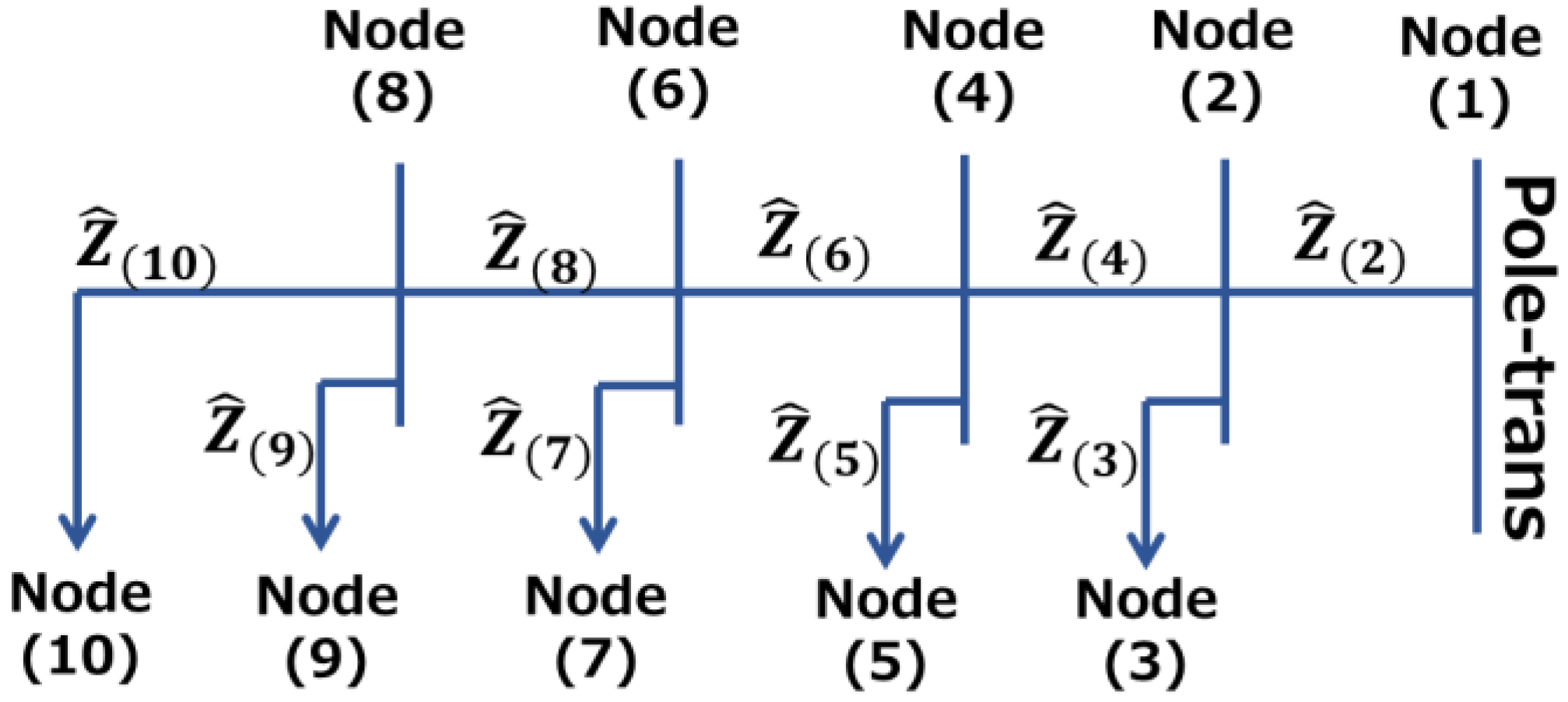
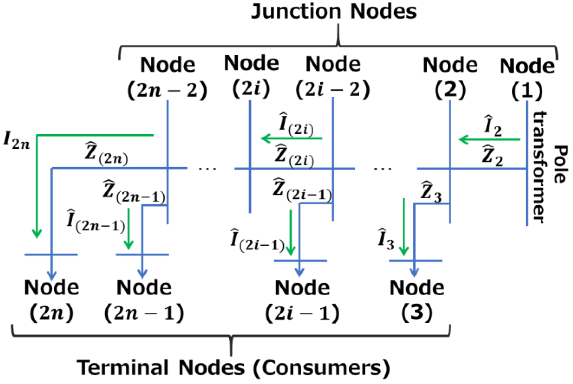
The rest of this paper is organized as follows: Section 2 elaborates on a model of a low-voltage distribution network and the modified equations used to estimate impedance. We describe a modified objective function used to estimate impedance and an enhanced PSO algorithm in Section 3. In Section 4, we show the effectiveness of the modified impedance estimation method through comparisons with a conventional impedance method.

2. Simulation Model

Figure 1 shows a typical distribution network that includes the connections of terminal consumers. Two kinds of nodes are shown in this figure: junction nodes (J-nodes) and terminal nodes (T-nodes). All T-nodes are at the ends of the branch and each T-node is connected to a household that consumes active and/or reactive power. J-nodes are connection points between each J-node and T-node, meaning that J-nodes do not directly connect to households. The configuration of the model starts from the first junction node that has a pole transformer and is named Node(1) and extends to the terminal nodes that are ends of a line. The model presented in this paper follows the assumptions below, the same premises upon which [17] is based:
  • The topology and order of all nodes are already known.
  • Every T-node where a consumer connects has a device, such as a smart meter, to measure the current, voltage, and power factor.
  • Each device indicates how much active and reactive power it consumes at any point in time, but cannot be exactly time synchronized across multiple consumers. Thus, information about phase differences between users cannot be shared.
  • Each device can measure and share only the rms values of voltage and current. The information measured by each device is shared among all consumers to enable impedance estimation.
In this model, the node numbers are incremented by one from Node(1). The supplied power flows from Node(1) to the farthest node named Node(2n). The range of i is 1 < in. The case where i = 1 is uniquely defined because this model uses a distance between Node(1) and Node(2) that considers the practical situation in the field. The conventional impedance estimation method in [17] expediently assumes that Node(1) has a T-node. However, it is more reasonable to use the distance from the node that has a pole transformer to the subsequent node. This paper proposes a method that estimates the expanded line between Node(1) and Node(2) in Figure 1. We make the following assumptions with respect to Node(1):
  • A device that measures current, voltage, and active and reactive power, including phase information, does not exist on Node(1).
  • The pole transformer properties are unknown, so the transformer’s secondary voltage is unknown, but is stable. Here “stable” implies that the voltage magnitude remains constant so that all devices can measure the voltage synchronously. Normally, one second would be enough of a window for this measurement since we are collecting only the rms voltage without its phase.
The discussion in [17] outlines the conventional formulation of equations used to obtain impedance. This paper details an improved formulation of impedance equations based on [17]. Each complex set of impedances is recurrently calculated starting from the case where i = n ( 2 n ) , the end of the network in Figure 1. We define this case as follows:
f ( 2 n ) ( Z ^ ( 2 n ) , Z ^ ( 2 n 1 ) ) = | V ( 2 n 1 ) | | V ( 2 n ) + Z ^ ( 2 n ) I ( 2 n ) Z ^ ( 2 n 1 ) I ^ ( 2 n 1 ) |
V ( 2 n ) is not expressed with “^” because the phase of V ( 2 n ) is zero; thus, V ( 2 n ) is the reference point for the other nodes from which current and voltage is determined. Also, I ( 2 n ) is not expressed with “^” because the current and voltage at each node is derived from the power that is measured at each node. I ^ ( 2 n 1 ) containing the phase difference observed from V ( 2 n ) cannot be measured directly. According to [17], I ^ ( 2 n 1 ) is expressed with impedances and known values as follows:
I ^ ( 2 n 1 ) = ( S ( 2 n ) + Z ^ ( 2 n ) | I ( 2 n ) | 2 + S ( 2 n 1 ) + Z ^ ( 2 n 1 ) | I ( 2 n 1 ) | 2 V ( 2 n ) + Z ^ ( 2 n ) I ( 2 n ) ) * I ( 2 n )
Equations (1) and (2) are expressed in known values, which can be measured. Next, we consider the following unconstrained minimization function:
m i n   f ( 2 n ) ( Z ^ ( 2 n ) , Z ^ ( 2 n 1 ) )
We determine the optimal complex solution set Z ^ ( 2 n ) and Z ^ ( 2 n 1 ) , which, if ideal, would make the function (3) zero. The details with respect to achieving the optimal solution are discussed in Section 4. Using the estimated Z ^ ( 2 n ) as (3), we obtain V ^ ( 2 n 2 ) as follows:
V ^ ( 2 n 2 ) = V 2 n + Z ^ ( 2 n ) I ( 2 n )
The case where i = 1 has a different equation than (1). The voltage V ^ ( 2 ) and current I ^ ( 2 ) injected into Node(2) are already calculated for the case where i = 1. The voltage on Node(1) is represented as follows:
V ^ ( 1   ) = V ^ ( 2 ) + Z ^ ( 2 ) I ^ ( 2 )
From (5), the function to obtain impedance Z ^ ( 2 ) is defined as follows:
f ( 1 ) ( Z ^ ( 2 ) ) = | V ^ ( 1   ) | | V ^ ( 2 ) + Z ^ ( 2 ) I ^ ( 2 ) |
In (6), | V ^ ( 1   ) | is assumed constant because it is defined as the voltage of the secondary side of a pole transformer. V ^ ( 2 ) and I ^ ( 2 ) including the phase difference from the other nodes are calculated based on the impedance, current, and voltage with reference to the case where i = 1. Now, the following unconstrained minimization problem is considered:
m i n   f ( 1 ) ( Z ^ ( 2 ) )
Z ^ ( 2 ) is obtained as the solution, which ideally makes (7) equal zero in the same way as (3). For the case where i = n − 1, Node(2n − 2) can be regarded as a node in the same way as Node(2n) because the current and voltage at Node(2n − 2) are already detailed in (4). All impedances can be recurrently calculated in the range of 2 i n . The following contributes to the work in [17]. According to (1), the function of Z ^ ( 2 i ) and Z ^ ( 2 i 1 ) is defined as:
f ( 2 i ) ( Z ^ ( 2 i ) , Z ^ ( 2 i 1 ) ) { | V ( 2 i 1 ) | | V ^ ( 2 i ) + Z ^ ( 2 i ) I ^ ( 2 i ) Z ^ ( 2 i 1 ) I ^ ( 2 i 1 ) | ,       2 i n | V ( 2 i 1 ) | | V ^ ( 2 i ) + Z ^ ( 2 i ) I ^ ( 2 i ) | ,       i = 1
Using (8), we can consider various load patterns. Load patterns at T-nodes are measured for all users at the same point in time. For example, when load patterns are acquired ten times, the ten patterns of measured voltage at Node(2i − 1) are expressed respectively as V ( 2 i 1 ) ( 1 ) ,   V ( 2 i 1 ) ( 2 )   V ( 2 i 1 ) ( 10 ) . The ten patterns of measured current and apparent power at Node(2i − 1) are expressed as I ( 2 i 1 ) ( 1 ) ,   I ( 2 i 1 ) ( 2 )   I ( 2 i 1 ) ( 10 ) and S ( 2 i 1 ) ( 1 ) ,   S ( 2 i 1 ) ( 2 )   S ( 2 i 1 ) ( 10 ) . Thus, (8) can be redefined for the jth load pattern as:
e ( i ) ( j ) = { | V ( 2 i 1 ) ( j ) | | V ^ ( 2 i ) ( j ) + Z ^ ( 2 i ) I ^ ( 2 i ) ( j ) Z ^ ( 2 i 1 ) I ^ ( 2 i 1 ) ( j ) | ,       2 i n | V ( 2 i 1 ) ( j ) | | V ^ ( 2 i ) ( j ) + Z ^ ( 2 i ) I ^ ( 2 i ) ( j ) | ,       i = 1
We define load patterns as lj, where j is the jth load pattern. e ( i ) ( j ) represents an error from load pattern l j . The conclusive cost function f ( 2 i ) ( Z ^ ( 2 i ) , Z ^ ( 2 i 1 ) ) , which should be minimized, is
f ( 2 i ) ( Z ^ ( 2 i ) , Z ^ ( 2 i 1 ) ) = m a x ( C ( e ( i ) ( j ) ) )
where categorized cost C ( e ( i ) ( j ) ) is defined as
C ( e ( i ) ( j ) ) =   { | e | ,       σ e σ e 4 ,       o t h e r w i s e
and
0 σ 1
In (9), each load pattern l j , produces an error e ( i ) ( j ) . Each error obtained from (9) is classified based on its range into a categorized cost C ( e ( i ) ( j ) ) . The maximum categorized cost obtained from the error list e ( i ) ( 1 ) , e ( i ) ( 2 ) e ( i ) ( x ) e ( i ) ( j ) is found alongside the xth load pattern l x that produced it as in (10). Tolerance σ can take any real value in the range shown in (12). Generally, the tolerance should be decided based on the requirements or restrictions of the problem. In this paper, we assume that the measuring devices at each T-node resolve two digits after the decimal point, so we take the tolerance σ to be 0.01.

3. The Enhanced PSO

In Section 2, we defined the conclusive cost functions in Equation (10). We now consider the following unconstrained minimization problem:
m i n   f ( 2 i ) ( Z ^ ( 2 i ) , Z ^ ( 2 i 1 ) )
The idea is to find the optimal complex solution set that provides a zero-cost value. According to the previous work in [17], the two functions that relate to the real and imaginary part of the power at T-node(2i) and T-node(2i − 1) are required to achieve this. In contrast, the new impedance estimation method we propose in this paper does not employ those functions.
In order to solve the optimization problem in (13), we implement an enhanced PSO algorithm. For this paper, the enhanced PSO was manually coded in Matlab rather than being implemented in packaged software. The original PSO algorithm is a well-known parallel evolutionary computation technique based on a social behavior metaphor [18]. The standard PSO algorithms mentioned in [19,20] are expressed as:
x ( k ) = c x ( k 1 ) + d v ( k )
v ( k ) = a v ( k 1 ) + b 1 r 1 ( P b e s t , ( k 1 ) x ( k 1 ) )   + b 2 r 2 ( G b e s t , ( k 1 ) x ( k 1 ) )
At iteration k, the velocity v ( k ) is updated based on its current value affected by a momentum factor a and on a term that attracts the particle towards previously found personal best P b e s t , ( k 1 ) and global best G b e s t , ( k 1 ) . One issue with PSO is how we select the coefficients a , b 1 , b 2 , c , and d . According to [20], the following assertions hold:
(1)
Coefficients b 1 and b 2 can be combined as b while maintaining the reliability of the model to obtain optimal solutions.
(2)
The coefficients a and b are major contributors to an optimal solution. The other coefficients c and d are fixed arbitrarily to enable the model to generalize.
Previous research shows that a value of inertia weight a between 0.4 and 0.9 yields the best results [21,22]. A larger value of inertia weight a is essential for a global search and a smaller value is essential for a local search. If we choose a larger value for inertia weight a , the PSO algorithm puts more emphasis on searching new areas rather than local areas. Hence, a PSO algorithm with a large inertia weight a might fail to find the optimal solution even though near to it. On the other hand, if a smaller value of inertia weight a is chosen, potential solutions could be limited to local solutions, which might be far from the optimal solution. The balance between global and local searches is critical in an attempt to find an optimal solution [23,24]. For these reasons, when the cost derived from a potential solution is still high, which means a potential solution is far from the true optimal solution, inertia weight a should be larger to search a larger area. On the other hand, when the cost is small, which means potential solutions are close to the true optimal solution, inertia weight a should be smaller to concentrate around the potential solutions.
The next problem is how to control the inertia weight a while considering the cost derived from potential solutions during each iteration. The cost function is nonlinear and is calculated by the proposed method in (11). Also, the cost may dynamically change during each iteration as shown in (10). Therefore, the inertia weights should be changed to reflect the cost during each iteration. Existing studies proposed some adaptive inertia weights [24,25,26,27]. All these studies modified adaptive inertia weights based on P b e s t and/or G b e s t at each iteration. In this paper, our objective is to estimate impedance with a small margin of error based on measured data at each secondary consuming node including consideration of measuring device accuracy. We use an adaptive inertia weight that is updated from the cost given by (11) at each iteration. We define the adaptive inertia weight as
a ( k ) = a m a x ( a m a x a m i n ) ϵ m a x ( ϵ , f ( 2 i ) ( Z ^ ( 2 i ) , Z ^ ( 2 i 1 ) ) )
where a ( k ) is the inertia weight at the kth iteration (updated for each iteration), ϵ is a constant defined as a criterion of cost, a m a x and a m i n are the maximum and minimum constants of inertia weight, f ( 2 i ) ( Z ^ ( 2 i ) , Z ^ ( 2 i 1 ) ) is the cost at the (k − 1)th iteration in (10). When the cost at the (k − 1)th iteration is larger than criterion ϵ , all potential solutions are still far from the optimal solution, with the result that the inertia weight at the kth iteration increases towards a m a x so that particles broaden their search space in search of the optimal solution. On the other hand, when the cost is smaller than criterion ϵ , potential solutions are near the optimal solution. As the cost decreases, the fractional part of (17) approaches a value of 1, and the inertia weight at the kth iteration approaches a m i n . In this paper, criterion ϵ is defined as 1, which is a hundred times the tolerance σ in (11), and a m a x and a m i n are defined as 0.9 and 0.4.

4. Case Study

In this case study, these T-nodes are defined: Node(3), Node(5), Node(7), Node(9) and Node(10). Each T-node has a measurement device that can measure voltage, current, and power consumption in synchronization with the others. (Note that phase level synchronization is not available). Internodal impedance is notated with a subscript. For example, the impedance between Node(2) and Node(1) is labeled Z ^ ( 2 ) .
The simulation procedure is as follows:
(1)
Power consumption is measured at each consuming node in time intervals as shown in Table 1. In this simulation, six consumption patterns (load patterns) are given. In a real situation, the number of the load patterns will be as many as needed because the consumption pattern will innately vary over time and the measuring devices continuously take data.
(2)
Voltage and current at each node are calculated based on Figure 2 using circuit theory with the respective load patterns, and these impedances are shown as actual impedances in Table 2.
(3)
Impedance is estimated without regard to phase differences of voltage and current between nodes since it is considered unknown. The impedances are estimated by recursively solving (13).
Previous estimation methods, as explained in [17], often cause errors in estimated impedance. Two concepts introduced herein improve the accuracy of the imaginary part of Z ^ ( 2 i ) and Z ^ ( 2 i 1 ) . The differences between the conventional method and the one proposed herein are:
(1)
The cost function in (11) reacts strongly when the error e is larger than 0.01.
(2)
The adaptive inertia weight a ( k ) in (16) improves the PSO algorithm accuracy.
Estimated impedances are the average of 50 estimates to verify the robustness of the PSO. The results from the PSO are not always the same given the same input data because of randomness derived from the PSO. In the PSO, the first potential solutions and inertia r 1 and r 2 in (15) are randomly selected in a specific range.
Figure 3 shows the estimation results from previous methods, the proposed method, and actual impedance calculations. The figure visualizes the results as indicated in the figure’s key with a whisker indicating the 95% confidence interval. In Figure 3a, the impedance real part estimate averages are acceptable and their confidence interval is very narrow. This narrow confidence interval provides a preferred estimate set. On the other hand, in Figure 3b, the previous method shows a wider confidence interval for imaginary part impedance than the proposed method, especially about Z ^ ( 7 ) and Z ^ ( 9 ) . The proposed method has a much smaller error than the previous method about Z ^ ( 3 ) ,   Z ^ ( 5 ) ,   Z ^ ( 7 ) , and Z ^ ( 9 ) .
The error between the estimated and actual impedance is shown in Figure 4. Figure 4a (real part) shows that in most cases the proposed method estimates impedances with a smaller error and narrower confidence interval than the previous method. Figure 4b (imaginary part) also shows that the proposed method estimates impedances with less error and a narrower confidence interval in all cases except for Z ^ ( 4 ) .
Table 2 shows the actual impedance, the estimated impedance from the previous method, and the estimated impedance from the proposed method. The estimated impedance is the average of the 50 simulations. The percentages in the estimated impedance indicate error rate compared with actual impedance. Re and Im are the real and imaginary impedance parts. As Table 2 shows, in most cases the estimated impedances using the proposed method are superior to the estimated impedance by the previous method. However, the proposed method also has a huge error rate in the imaginary part of Z ^ ( 5 ) and Z ^ ( 7 ) , which is visualized in Figure 4b as the gap between the actual and estimated impedance. In Figure 4b, the confidence intervals of Z ^ ( 5 ) and Z ^ ( 7 ) estimated by the proposed method are wider than the other parts. This means that the solution provided by the proposed PSO algorithm varies at every estimation. Two causes can be considered: the parameters such as weights for the velocity of the PSO are not appropriately tuned up, or some different solution sets can be the global optimal solution to minimize the cost of the objective function. The first cause can be rejected because the other parts, such as the imaginary part of Z ^ ( 3 ) and Z ^ ( 9 ) , show a reasonable error rate in Table 2. If the parameters are not properly adjusted, the other parts should also have the error as the imaginary part of Z ^ ( 5 ) and Z ^ ( 7 ) . The second cause mentioned above may be the combination of load patterns as in Table 1. The load patterns form non-linear simultaneous equations to solve the PSO, but some of the simultaneous equations can be very similar because similar load patterns derive similar equations. This problem can be solved by collecting enough measurements for load patterns.

5. Conclusions

This paper proposed an improved impedance estimation method for low-voltage distribution feeders. The proposed method overcomes three problems in existing impedance estimation methods for a low-voltage network: time synchronized measurement, a generalization of the network model, and convergence of the optimization. The previous method, which can deal with non-synchronized measurement data, is improved in this paper. A generalized network model that considers the distance between the pole transformers and inter-connecting nodes has been adopted. The formulation for a generalized model has also been developed. A conventional PSO algorithm was modified by employing an adaptive inertia weight. The accuracy of the impedance estimation was validated in the case study as follows:
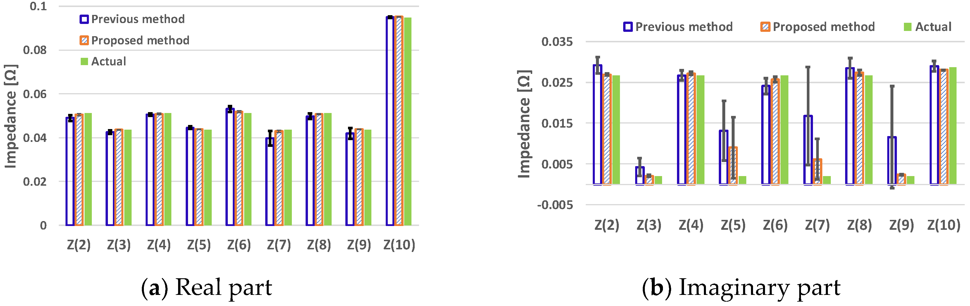
  • The proposed method estimates an extended part of the low-voltage distribution feeder, Z ^ ( 2 ) , with reasonable error. The average error rate of the real part was 1.4% and that of the imaginary part was 0.8%.
  • The proposed method estimates impedance as well as or better than the previous method in terms of estimation average and confidence intervals of the estimation.
  • The proposed method still has a huge error rate on the imaginary part of Z ^ ( 5 ) and Z ^ ( 7 ) even though the accuracy is improved over the previous method. The appropriate load patterns are needed to obtain better accuracy on Z ^ ( 5 ) and Z ^ ( 7 ) .
The proposed impedance estimation scheme would be helpful for developing new applications such as voltage regulation using DERs.

Author Contributions

S.H. (Sekyung Han) and S.H. (Soohee Han) conceived of the presented idea. D.K., J.P. and S.Y.K. developed the theory and performed the computations. S.H. (Sekyung Han) supervised the findings of this work. All authors discussed the results and contributed to the final manuscript.

Funding

This work was supported by the National Research Foundation of Korea (NRF) grant funded by the Korea government (MSIT) (No.2017R1A1A1A05001357).

Conflicts of Interest

The authors declare no conflict of interest.

Nomenclature

The symbols that are expressed with ‘^’ mean that they are not measurable directly with equipment.
nreal number, 2 ≤ n
ian index of nodes, 1 ≤ in
V ^ ( 2 i ) node voltage at Node(2i)
I ^ ( 2 i ) line current injected to Node(2i) from Node(2i − 2)
S ^ ( 2 i ) injected apparent power to Node(2i)
Z ^ ( 2 i ) impedance between Node(2i) and Node(2i − 2)

References

  1. Liu, E.; Bebic, J. Distribution system voltage performance analysis for high-penetration photovoltaics distribution system voltage performance analysis for high-penetration photovoltaics. In Proceedings of the 2008 IEEE Energy 2030 Conference, Atlanta, GA, USA, 17–18 November 2008. [Google Scholar]
  2. Kordkheili, R.A.; Bak-Jensen, B.; R-Pillai, J.; Mahat, P. Determining maximum photovoltaic penetration in a distribution grid considering grid operation limits. In Proceedings of the 2014 IEEE PES General Meeting Conference Exposition, National Harbor, MD, USA, 27–31 July 2014; pp. 1–5. [Google Scholar]
  3. Masters, C.L. Voltage rise: The big issue when connecting embedded generation to long 11 kV overhead lines. Power Eng. J. 2002, 16, 5–12. [Google Scholar] [CrossRef]
  4. Kabiri, R.; Holmes, D.G.; McGrath, B.P.; Meegahapola, L.G. LV grid voltage regulation using transformer electronic tap changing, with pv inverter reactive power injection. IEEE J. Emerg. Sel. Top. Power Electron. 2015, 3, 1182–1192. [Google Scholar] [CrossRef]
  5. Salih, S.N.; Chen, P. On coordinated control of OLTC and reactive power compensation for voltage regulation in distribution systems with wind power. IEEE Trans. Power Syst. 2015, 31, 4026–4035. [Google Scholar] [CrossRef]
  6. Vovos, P.N.; Kiprakis, A.E.; Wallace, A.R.; Harrison, G.P. Centralized and distributed voltage control: Impact on distributed generation penetration. IEEE Trans. Power Syst. 2007, 22, 476–483. [Google Scholar] [CrossRef]
  7. Demirok, E.; González, P.C.; Frederiksen, K.H.B.; Sera, D.; Rodriguez, P.; Teodorescu, R. Local reactive power control methods for overvoltage prevention of distributed solar inverters in low-voltage grids. IEEE J. Photovolt. 2011, 1, 174–182. [Google Scholar] [CrossRef]
  8. Dall’Anese, E.; Dhople, S.V.; Giannakis, G.B. Optimal dispatch of photovoltaic inverters in residential distribution systems. IEEE Trans. Sust. Energy 2014, 5, 487–497. [Google Scholar] [CrossRef]
  9. Dall’Anese, E.; Dhople, S.V.; Giannakis, G.B. Decentralized optimal dispatch of photovoltaic inverters in residential distribution systems. IEEE Trans. Sust. Energy 2014, 29, 957–967. [Google Scholar] [CrossRef]
  10. Elkhatib, M.E.; El-Shatshat, R.; Salama, M.M.A. Novel coordinated voltage control for smart distribution networks with DG. IEEE Trans. Smart Grid 2011, 2, 598–605. [Google Scholar] [CrossRef]
  11. Marra, F.; Yang, G.Y.; Traeholt, C.; Larsen, E.; Ostergaard, J.; Blazic, B.; Deprez, W. EV charging facilities and their application in LV feeders with photovoltaics. IEEE Trans. Smart Grid 2013, 4, 1533–1540. [Google Scholar] [CrossRef]
  12. Peppanen, J.; Reno, M.J.; Broderick, R.J.; Grijalva, S. Distribution system model calibration with big data from AMI and PV inverters. IEEE Trans. Smart Grid 2016, 7, 2497–2506. [Google Scholar] [CrossRef]
  13. Castillo, M.R.M.; London, J.B.A.; Bretas, N.G. Network branch parameter validation based on a decoupled state/parameter estimator and historical data. In Proceedings of the 2009 IEEE Bucharest, Bucharest, Romania, 28 June–2 July 2009. [Google Scholar]
  14. Castillo, M.R.M.; London, J.B.A.; Bretas, N.G. An approach to power system branch parameter estimation. In Proceedings of the 2008 IEEE Electric Power Energy Conference, Vancouver, BC, Canada, 6–7 October 2008. [Google Scholar]
  15. Wu, Z.; Zora, L.T.; Phadke, A.G. Simultaneous transmission line parameter and PMU measurement calibration. In Proceedings of the IEEE Power & Energy Society General Meeting, Denver, CO, USA, 26–30 July 2015. [Google Scholar]
  16. Berrisford, A.J. A tale of two transformers: An algorithm for estimating distribution secondary electric parameters using smart meter data. In Proceedings of the 26th IEEE Canadian Conference on Electrical and Computer Engineering (CCECE), Regina, SK, Canada, 5–8 May 2013. [Google Scholar]
  17. Han, S.; Kodaira, D.; Han, S.; Kwon, B.; Hasegawa, Y.; Aki, H. An automated impedance estimation method in low-voltage distribution network for coordinated voltage regulation. IEEE Trans. Smart Grid 2016, 7, 1012–1020. [Google Scholar] [CrossRef]
  18. Kennedy, J.; Eberhart, R. Particle swarm optimization. In Proceedings of the Sixth International Symposium on Micro Machine and Human Science, Nagoya, Japan, 6 August 2002. [Google Scholar]
  19. Han, S.; Kodaira, D.; Han, S.; Baek, J. Practical impedance estimation in low-voltage distribution network. IFAC-PapersOnLine 2015, 48, 312–315. [Google Scholar] [CrossRef]
  20. Trelea, I.C. The particle swarm optimization algorithm: Convergence analysis and parameter selection. Inf. Process. Lett. 2003, 85, 317–325. [Google Scholar] [CrossRef]
  21. Eberhart, R.C.; Shi, Y. Comparing inertia weights and constriction factors in particle swarm optimization. In Proceedings of the 2000 Congress on Evolutionary Computation, La Jolla, CA, USA, 16–19 July 2000. [Google Scholar]
  22. Črepinšek, M.; Liu, S.-H.; Mernik, M. Exploration and exploitation in evolutionary algorithms. ACM Comput. Surv. 2013, 45, 1–33. [Google Scholar] [CrossRef]
  23. Eberhart, R.C. Fuzzy adaptive particle swarm optimization. In Proceedings of the 2001 Congress on Evolutionary Computation, Seoul, Korea, 27–30 May 2001. [Google Scholar]
  24. Taherkhani, M.; Safabakhsh, R. A novel stability-based adaptive inertia weight for particle swarm optimization. Appl. Soft Comput. 2016, 38, 281–295. [Google Scholar] [CrossRef]
  25. Nickabadi, A.; Ebadzadeh, M.M.; Safabakhsh, R. A novel particle swarm optimization algorithm with adaptive inertia weight. Appl. Soft Comput. J. 2011, 11, 3658–3670. [Google Scholar] [CrossRef]
  26. Yang, X.; Yuan, J.; Yuan, J.; Mao, H. A modified particle swarm optimizer with dynamic adaptation. Appl. Math. Comput. 2007, 189, 1205–1213. [Google Scholar] [CrossRef]
  27. Arumugam, M.S.; Rao, M.V.C. On the improved performances of the particle swarm optimization algorithms with adaptive parameters, cross-over operators and root mean square (RMS) variants for computing optimal control of a class of hybrid systems. Appl. Soft Comput. J. 2008, 8, 324–336. [Google Scholar] [CrossRef]
Figure 1. Simulation model: generalized linear Low-Voltage distribution network.
Energies 12 01167 g001
Figure 2. Five T-nodes in the model for the case study.
Energies 12 01167 g002
Figure 3. Average and 95% confidence interval for estimated impedance (real and imaginary part).
Energies 12 01167 g003
Figure 4. Average and 95% confidence interval for error of estimated impedance (real and imaginary part).
Energies 12 01167 g004
Table 1. Six load patterns at each node including active and reactive power.
Load
Pattern
S(3)
[KVA]
S(5)
[KVA]
S(7)
[KVA]
S(9)
[KVA]
S(10)
[KVA]
#12.00 + 0.15i2.00 + 0.10i2.50 + 0.30i2.00 + 1.00i0.50 + 0.30i
#21.00 + 0.40i3.00 + 0.50i1.00 + 0.20i2.70 + 1.50i0.50 + 0.30i
#30.80 + 0.30i1.50 + 0.20i0.70 + 0.10i1.20 + 0.30i0.40 + 0.20i
#40.30 + 0.15i1.30 + 0.20i1.10 + 0.30i3.10 + 0.30i0.35 + 0.20i
#51.25 + 0.13i0.55 + 0.26i1.34 + 0.45i2.30 + 1.30i0.35 + 0.20i
#61.00 + 0.15i1.10 + 0.20i0.30 + 0.05i3.50 + 2.10i0.60 + 0.35i
Table 2. Simulation result of impedance estimation.
ImpedanceActual
[Ω]
Average of Estimates by Previous Method
[Ω]
Average of Estimates by Proposed Method
[Ω]
ReImReImReIm
Z ^ ( 2 ) 0.05120.02670.0489
(4.5%)
0.0292
(9.5%)
0.0504
(1.4%)
0.0269
(0.8%)
Z ^ ( 3 ) 0.04360.00200.0425
(2.4%)
0.0042
(105.5%)
0.0435
(0.1%)
0.0020
(1.3%)
Z ^ ( 4 ) 0.05120.02670.0505
(1.3%)
0.0266
(0.0%)
0.0508
(0.8%)
0.0271
(1.8%)
Z ^ ( 5 ) 0.04360.00200.0445
(2.2%)
0.0131
(536.0%)
0.0437
(0.3%)
0.0089
(336.2%)
Z ^ ( 6 ) 0.05120.02670.0530
(3.6%)
0.0240
(9.9%)
0.0518
(1.3%)
0.0257
(3.7%)
Z ^ ( 7 ) 0.04360.00200.0396
(9.0%)
0.0166
(710.0%)
0.0429
(1.6%)
0.0061
(199.0%)
Z ^ ( 8 ) 0.05120.02670.0497
(2.9%)
0.0284
(6.7%)
0.0507
(0.8%)
0.0273
(2.5%)
Z ^ ( 9 ) 0.04360.00200.0419
(3.8%)
0.0115
(461.2%)
0.0437
(0.3%)
0.0023
(12.2%)
Z ^ ( 10 ) 0.09480.02870.0950
(0.3%)
0.0289
(0.7%)
0.0952
(0.5%)
0.0280
(2.4%)

