A Power Exchange Strategy for Multiple Areas with Hydro Power and Flexible Loads

Abstract

Areas with hydro power may purchase extra power from the outside power market during dry seasons, which will cause a deviation between the actual and expected power purchase amount due to the inaccurate judgment of the market situation. Because of the uncertainty of price fluctuations, the risk of purchasing power in the real-time market to eliminate this deviation is very high. This paper proposes an innovative trade mode, where the power exchange strategy between multiple areas is adopted through forming an alliance, i.e., one area can use the controllable elements within others, and constructing a monthly and post day-ahead two phase optimization model. The objective function of the monthly stochastic robust optimization considers the power purchase cost to determine the controllable elements dispatch dates for every area in the alliance. Thus, areas can make reasonable dispatch schedules for controllable elements to avoid the resource waste that means more controllable elements are prepared before post day-ahead optimization but less are used after post day-ahead optimization. While the post day-ahead optimization model determines the internal controllable elements dispatch and power exchange amount after the day-ahead market clearing process, users’ satisfaction and dispatch schedule changes for energy storage device are also considered. In order to solve the proposed two phase model, the dual principle and linearization methods are used to convert them into mixed-integer linear programming problems that can be effectively solved by the Cplex solver. The study case verifies the power deviation cost decreases with the power exchange strategy and the important role of energy storage devices.

1. Introduction

In western China, there are many adjacent areas with hydro power plants that supply the local loads. In general, a large hydro plant can prepare its own daily generation schedule [1]. However, because the hydro power is not sufficient in dry seasons and most of these areas only have small run-off type hydro power with poor regulation ability [2], they need to purchase extra power from the outside power market through brokers. Since the brokers are characterized as immature, they may make an inaccurate judgment about the day-ahead market situation and there will be a deviation between the actual and expected power purchase amount after the market’s clearing process [3,4]. Then, the brokers will generally purchase electricity power in the real-time market. However, the price fluctuations in real-time market are usually higher than those in the day-ahead market, thus the whole power purchase cost for brokers may increase greatly.

In general, the controllable elements, such as energy storage devices, and flexible loads (interruptible/transferable) with demand response capability, will be dispatched to eliminate this power purchase deviation post day-ahead. In [5], a monthly energy deviation trade mode with the participation of interruptible loads was established. In [6], a bi-level model of electricity purchase and sale strategies for brokers was proposed by taking user’s demand response technology into account. The brokers utilized a short-term demand response to avoid power unbalances and reduce the power purchase risk. A stochastic optimization model to maximize the broker’s profit was established in [7], where the stepwise reward-based demand response was considered. In [8], a bidding strategy model for brokers participating in the day-ahead market was proposed based on the aggregated household demand response. However, all these studies mainly use demand response to cut down peak loads and shift them to off-peaks and ignore the feasibility of applying a power exchange strategy, i.e., where one area can use the controllable elements within another area, to eliminate the power purchase deviations occurred in the day-ahead market.

Because most areas with hydro power plants are adjacent, a power exchange strategy between multiple area brokers to eliminate the positive or negative power purchase deviations for areas participating in this power exchange strategy is presented in this paper. A positive power purchase deviation represents the situation where the actual amount of power purchased is higher than the expected in order to motivate users to consumer more power, while a negative deviation means that the actual power purchase amount is lower than the expected one. An alliance is formed by the areas involved in the power exchange strategy. Moreover, if the brokers only perform a post day-ahead optimization, resource waste, which means controllable elements prepare more before optimization but use less after optimization will often occur, so the monthly optimization to determine the days that controllable elements are dispatched is necessary. After the day-ahead market clearing process, the brokers need to re-optimize based on the monthly optimization results to obtain the power exchange amount and cost.

To date, a number of studies have been done on power exchange strategies. In [9,10], a demand response exchange model was both applied to managing the variability of renewable energy sources. In [11], an energy exchange strategy between electric vehicle loads and wind generation utilities was built to mitigate wind energy and electric vehicle imbalance threats. In [12], a power exchange strategy was adopted to eliminate the power purchase deviations occurring in a day-ahead market, but only the interruptible load was used as controllable element. In addition, the optimization model only covered the post day-ahead process, while neglecting the monthly optimization. The main contributions of the paper can be summarized as follows:

(1)

A power exchange strategy between multiple areas is proposed so that these areas could reduce the positive and negative power purchase deviations in the day-ahead market, respectively. Areas can also borrow others’ controllable elements by using the power exchange strategy to avoid resource waste.

(2)

Bi-level monthly optimization which describes uncertain spot market prices as a robust variable could guide the areas on how to configure the dispatch schedule of controllable elements. Post day-ahead optimization provides areas with a dynamic adjustment strategy as time approaches.

(3)

Both monthly and post day-ahead optimization models are mixed-integer linear programming problems which can be efficiently solved by the Cplex solver using the dual-principle and linearization methods.

The rest of this paper is organized as follows: Section 2 describes the power exchange strategy mechanism. Section 3 presents the monthly and post day-ahead optimization model, respectively. In Section 4, the algorithm for optimization is proposed. In Section 5, numerical case studies verify the effectiveness of the proposed model. The conclusions are given in Section 6.

2. Power Exchange Strategy among Areas

The areas in the alliance can eliminate the power purchase deviations occurring in the day-ahead market mainly through two ways, i.e., dispatching their internal controllable elements and adopting a power exchange strategy. After the day-ahead market clearing, i.e., post day-ahead market, the brokers firstly dispatch their internal controllable elements to meet their own demand, and then can lend an extra available controllable elements to other brokers through the power exchange strategy. All brokers should pay the power exchange center a fee for the grid congestion caused by the power exchange.

In this paper, within one area, the controllable elements include pumped storage hydro power stations and flexible loads with demand response ability such as interruptible loads and transferable loads. The charging and discharging energy of a pumped storage power station can be lent to other brokers through adjusting the water level. Different types of demand response capability have different power exchange strategies: (i) for interruptible loads, a broker with positive deviation can lend this extra power, by interrupting its load, to the broker who has a negative deviation, (ii) for transferable loads, if there are two brokers with opposite deviations in different periods, the broker with positive deviation could transfer the load to make opposite deviations occur in the same period, thus the opposite deviations could be eliminated. The power exchange from broker A with positive deviation to broker B with negative deviation is shown in Figure 1, where the load reduction of broker A is realized through load interruption and transfer, as well as the decreased power output of the pumped storage power station.

The power exchange strategy should cover monthly and post day-ahead two phase optimization. If the brokers only perform a post day-ahead optimization, resource waste, which means more controllable elements are prepared before optimization but less used after optimization will often occur.

Firstly, the area needs to participate in the medium and long-term market at the end of each month, so after the monthly market clears up, the area allocates its controllable resources reasonably to reduce the spot risk in the spot market.

Secondly, the power generation of hydropower is affected by the incoming water, and the past incoming water over the years plays a supporting role in the prediction of hydropower.

Besides, the monthly optimization could decrease the number of times controllable elements are dispatched unnecessarily. Thus, the capacity cost for loads with demand response capability will decrease and the lifespan of energy storage equipment will increase.

Moreover, the user’s satisfaction and willingness of signing a demand response contract again would be enhanced. Therefore, the monthly optimization to determine the controllable elements dispatch date is necessary.

After day-ahead market clearing, the power purchase amount and price for areas are both determined. If there exists a power purchase deviation, the proposed post day-ahead optimization starts in order to derive the power exchange amount and cost based on the above monthly optimization results.

Thus, the power exchange strategy among areas proposed in this paper could be divided into two phases. In the monthly phase, the controllable element dispatch dates, i.e., whether they are available every day or not, can be determined. In the post day-ahead phase, because the schedulable or not status of controllable elements is clearly known, the internal and exchange controllable element dispatch amount can both be obtained.

The monthly optimization result is shown in Figure 2, where the circles represent controllable elements. The orange ones indicate the controllable element could be dispatched while the white ones indicate it could not be dispatched.

3. Two Phase Modeling

3.1. Uncertain Variable

In the monthly optimization model, the power purchase amount and price in the day-ahead market are both uncertain variables, which can be obtained in many ways as follows:

(1)

Stochastic optimization [13], in which uncertain variables are described as probability distribution functions. For instance, in [14], according to the bid curve of other market participants, the power purchase strategy for a large consumer was derived by stochastic optimization. In [15], the load and distributed sources power quantity uncertainty were shown by scenario analysis, thus a stochastic dispatch model was established.

(2)

Robust optimization, in which uncertain variables are described as robust variables within a certain confidence interval, only taking the worst fluctuation of uncertain variables into account. For instance, in [16], a day-ahead market bidding model was established through robust optimization, in which the market price mechanism was built.

(3)

Information gap decision making theory [17,18], in which the decision-making risk was considered by means of uncertain variables.

(4)

Sequential simulation [19], in which the uncertain variables were simulated according to their historical data.

It is not easy to describe the power purchase price in the day-ahead market according to its probability distribution function since it is affected by the decisions of all brokers participating in market. In order to illustrate the severity of the market price, the spot market price can be described as a robust variable. Because the power purchase amount is related to the bidding decisions of the brokers, it can be described as a stochastic variable according to historical data to get its fluctuation characteristics relative to the load curve.

3.2. Monthly Robust Stochastic Optimization

The output result of monthly optimization is whether all kinds of controllable elements are allocated in 30 days. The objective function of optimization includes three parts. One is the expected cost of controllable elements, which includes the reserve capacity cost and the expected value of the daily cost in each scenario. The second is the expected cost of the power exchange strategy to each other. The third is the expected value of the day-ahead and real-time electricity purchase cost.

In the electricity price part, it is described as a robustness variable, so a robust optimization model is used to make the above optimization under certain adverse electricity price conditions andma typical min max robust optimization model is established.

The objective function of monthly optimization is the minimum expected cost for every area as follows:

$$\begin{array}{l}{\min }_{{\theta }_{t,s,d}^C\in \alpha }{\max }_{C_{d,t}^{\mathrm{da}}\in \lambda }{\displaystyle \sum _{i,d,k}(C_{i,u}^k{U}_{i,d}^k)}+{\displaystyle \sum _s\left\{P_s\times \right.}{\displaystyle \sum _i{\displaystyle \sum _d\left[{\displaystyle \sum _t{C}_{i,t}^{\mathrm{I}}{L}_{i,s,d,t}^{\mathrm{I}}}+{\displaystyle \sum _{t_1\ne t_2}{C}_{i,t}^{\mathrm{Sh}}{L}_{i,s,d,t_1,t_2}^{\mathrm{Sh}}}\right.}}\\ +C_{i,t}^{\mathrm{Ec}}{L}_{i,s,d,t}^{\mathrm{Ec}}+C_{i,t}^{\mathrm{Ed}}{L}_{i,s,d,t}^{\mathrm{Ed}}+{\displaystyle \sum _{j\ne i}{C}_{\mathit{ij},t}^{\mathrm{Tr}}(L_{\mathit{ji},d,t,s}^{\mathrm{Tr}}+}\left.\left.L_{\mathit{ij},d,t,s}^{\mathrm{Tr}})+C_{d,t}^{\mathrm{da}}{L}_{i,s,d,t}^{\mathrm{da}}+C_{d,t}^{\mathrm{rt}}{L}_{i,s,d,t}^{\mathrm{rt}}\right]\Delta t\right\}\end{array}$$

(1)

where s, i, d, t, k are the indexes of scenarios, areas, dates, time periods and controllable elements, respectively;$\Delta t$ is the time interval between adjacent periods; $C_{i,u}^k$, $U_{i,d}^k$ are the reserve cost and state of controllable elements k within area i in day d; $P^S$ is the probability of scenario s; $C_{i,t}^{\mathrm{I}}$, $L_{i,s,d,t}^{\mathrm{I}}$ are the cost and value of the interruptible load within area i; $C_{i,t}^{\mathrm{Sh}}$, $L_{i,s,d,t_1,t_2}^{\mathrm{Sh}}$ are the cost and value of the transferable load within area i from time t₁ to t₂; $L_{i,s,d,t}^{\mathrm{Ed}}$, $L_{i,s,d,t}^{\mathrm{Ec}}$, $C_{i,t}^{\mathrm{Ed}}$, $C_{i,t}^{\mathrm{Ec}}$ are the discharging and charging energy and cost of energy storage equipment within area i; $C_{ij,t}^{\mathrm{Tr}}$ is the power exchange cost between area i and j; $L_{ij,d,t,s}^{\mathrm{Tr}}$ is the power exchange amount from area i to j; $L_{i,s,d,t}^{\mathrm{da}}$, $L_{i,s,d,t}^{\mathrm{rt}}$, $C_{d,t}^{\mathrm{da}}$, $C_{d,t}^{\mathrm{rt}}$ are the day-ahead and real-time market power purchase amount and price, respectively.

The objective Equation (1) can be divided into two levels. The decision variable in the upper level is the stochastic variable described as follows:

$${\theta }_{t,s,d}^C=\left\{\begin{array}{l}{U}_{i,d}^k,L_{i,s,d,t}^{\mathrm{I}},L_{i,s,d,t_1,t_2}^{\mathrm{Sh}},L_{i,s,d,t}^{\mathrm{Ec}},\\ L_{i,s,d,t}^{\mathrm{Ed}},L_{\mathit{ji},d,t,s}^{\mathrm{Tr}},L_{\mathit{ij},d,t,s}^{\mathrm{Tr}},L_{i,s,d,t}^{\mathrm{rt}}\end{array}\right\}$$

(2)

The decision variables in the lower level are the worst day-ahead market price $C_{d,t}^{\mathrm{da}}$ and real-time market price $C_{d,t}^{\mathrm{rt}}$, which make the brokers’ power purchase cost the highest.

In the monthly optimization objective function, the first part represents the reserve cost for all kinds of controllable elements, the second and third parts stand for the dispatch costs of interruptible and transferrable loads, respectively, the fourth and fifth parts are charging and discharging cost of energy storage, the sixth part is the power exchange cost, and the last two parts are day-ahead market and real-time market power purchase cost, respectively.

The constraints of monthly optimization are as follows:

The first indicates interruptible load constraint:

$$u_{i,s,d,t}^{\mathrm{I}}{L}_{i,\min }^{\mathrm{I}}<=L_{i,s,d,t}^{\mathrm{I}}<=u_{i,s,d,t}^{\mathrm{I}}{L}_{i,\max }^{\mathrm{I}}$$

(3)

$$S_{\mathrm{on},i,s,d,t}^{\mathrm{I}}=(S_{\mathrm{on},i,s,d,t-1}^{\mathrm{I}}+1-u_{i,s,d,t}^{\mathrm{I}})\times (1-u_{i,s,d,t}^{\mathrm{I}})$$

(4)

$$S_{\mathrm{off},i,s,d,t}^{\mathrm{I}}=(S_{\mathrm{off},i,s,d,t-1}^{\mathrm{I}}+u_{i,s,d,t}^{\mathrm{I}})\times u_{i,s,d,t}^{\mathrm{I}}$$

(5)

$$\left\{\begin{array}{c}0\le (u_{i,s,d,t-1}^{\mathrm{I}}-u_{i,s,d,t}^{\mathrm{I}})\times (S_{\mathrm{on},i,s,d,t}^{\mathrm{I}}-T_{i,\mathrm{on}}^{\mathrm{I}}) \forall t>1\\ 0\le (u_{i,s,d-1,T}^{\mathrm{I}}-u_{i,s,d,t}^{\mathrm{I}})\times (S_{\mathrm{on},i,s,d,t}^{\mathrm{I}}-T_{i,\mathrm{on}}^{\mathrm{I}}) \forall t=1\end{array}\right.$$

(6)

$$\left\{\begin{array}{c}0\le (u_{i,s,d,t}^{\mathrm{I}}-u_{i,s,d,t-1}^{\mathrm{I}})\times (S_{\mathrm{off},i,s,d,t}^{\mathrm{I}}-T_{i,\mathrm{off}}^{\mathrm{I}}) \forall t>1\\ 0\le (u_{i,s,d,t}^{\mathrm{I}}-u_{i,s,d-1,T}^{\mathrm{I}})\times (S_{\mathrm{off},i,s,d,t}^{\mathrm{I}}-T_{i,\mathrm{off}}^{\mathrm{I}}) \forall t=1\end{array}\right.$$

(7)

The constraints from Equations (3) to (6) are related to the interruptible load. In order to avoid causing inconveniences to users, the minimum and maximum interruptible load values $L_{i,\min }^{\mathrm{I}}$, $L_{i,\max }^{\mathrm{I}}$ within area i are set in Equation (3), where $u_{i,s,d,t}^{\mathrm{I}}$ is the state vector, while $u_{i,s,d,t}^{\mathrm{I}}=1$ means the interruptible load of area i is dispatched in scenario sat time t in day d and $u_{i,s,d,t}^{\mathrm{I}}=0$ means it not dispatched. In order to avoid too frequent startup/shutdown switching and increase load equipment’s lifespan, the variables $S_{\mathrm{on},i,s,d,t}^{\mathrm{I}}$ and $S_{\mathrm{off},i,s,d,t}^{\mathrm{I}}$ are firstly introduced as a continuous interrupted and non-interrupted time in Equations (4) and (5), respectively. Then, the first constraints in Equations (6) and (7) represent in the intra-day a load should be kept on/off for at least $T_{i,\mathrm{off}}^{\mathrm{I}}$/$T_{i,\mathrm{on}}^{\mathrm{I}}$ continuous time before it can be turned off/on, where $T_{i,\mathrm{on}}^{\mathrm{I}}$ and $T_{i,\mathrm{off}}^{\mathrm{I}}$ are maximum continuous interruption and operation time. The second constraints in Equations (6) and (7) represent in the inter-day a load should meet the maximum continuous interruption and operation time requirement.

Then the constraints of transferable loads are as follows:

$$0<={\displaystyle \sum _{t_2}{L}_{i,s,d,t,t_2}^{\mathrm{Sh}}}<=L_{i,s,d,t,\max }^{\mathrm{Sh}}$$

(8)

$$L_{i,s,d,t,t_2}^{\mathrm{Sh}}=0\hspace{1em}\forall \left|t_2-t\right|>=t_{\mathrm{Sh}}$$

(9)

The constraint (8) is the limit of transferrable load, where $L_{i,s,d,t,\max }^{\mathrm{Sh}}$ is the upper limit in a time period. In order to enhance users’ satisfaction, Equation (9) represents that the transfer time should not be too long, where $t_{\mathrm{Sh}}$ is the maximum transferrable time.

Then energy storage constraints are shown as follows:

$$0<=L_{i,s,d,t}^{\mathrm{Ec}}<=u_{i,s,d,t}^{\mathrm{Ec}}{L}_{i,s,\max }^{\mathrm{Ec}}$$

(10)

$$0<=L_{i,s,d,t}^{\mathrm{Ed}}<=u_{i,s,d,t}^{\mathrm{Ed}}{L}_{i,s,\max }^{\mathrm{Ed}}$$

(11)

$$E_{i,s,d,t}^{\mathrm{ESS}}=E_{i,s,d,t-1}^{\mathrm{ESS}}+r_i^{\mathrm{c}}{L}_{i,s,d,t}^{\mathrm{Ec}}-r_i^{\mathrm{d}}{L}_{i,s,d,t}^{\mathrm{Ed}}$$

(12)

$$0<=E_{i,s,d,t}^{\mathrm{ESS}}<=E_{i,\max }^{\mathrm{ESS}}$$

(13)

$$u_{i,s,d,t}^{\mathrm{Ec}}+u_{i,s,d,t}^{\mathrm{Ed}}<=1$$

(14)

$$E_{i,s,d,1}^{\mathrm{ESS}}=E_{i,s,d-1,24}^{\mathrm{ESS}}$$

(15)

The constraints from Equations (10) to (15) are related to energy storage. Equations (10) and (11) are the upper limit of charging and discharging energy, where $u_{i,s,d,t}^{\mathrm{Ec}}$, $u_{i,s,d,t}^{\mathrm{Ed}}$ and $L_{i,s,\max }^{\mathrm{Ec}}$, $L_{i,s,\max }^{\mathrm{ED}}$ are the state variables and limits. Equation (12) represents the power balance equation between adjacent periods, where $r_i^{\mathrm{c}}$ and $r_i^{\mathrm{d}}$ are the charging and discharging efficiency, respectively. Equation (13) is the limit $E_{i,\max }^{\mathrm{ESS}}$ for storage energy in every time period. Equation (14) represents that the charging and discharging state cannot happen simultaneously. Equation (15) represents the initial stored energy in day d equals to the energy in the last time period in previous day (d-1), which makes sure that energy storage can be continuously utilized every day.

The fourth part is the constraints of electricity transfer, as shown below:

$$0<=L_{\mathit{ji},d,t,s}^{\mathrm{Tr}}<=u_{\mathit{ji},d,t,s}^{\mathrm{de}}{L}_{\mathit{ji},\max }^{\mathrm{Tr}}$$

(16)

$$0<=L_{\mathit{ij},d,t,s}^{\mathrm{Tr}}<=u_{\mathit{ij},d,t,s}^{\mathrm{de}}{L}_{\mathit{ij},\max }^{\mathrm{Tr}}$$

(17)

$$u_{\mathit{ji},d,t,s}^{\mathrm{de}}+u_{\mathit{ij},d,t,s}^{\mathrm{de}}<=1$$

(18)

$$\begin{array}{c}{L}_{i,s,d,t}^{\mathrm{da}}+L_{i,s,d,t}^{\mathrm{rt}}+{\displaystyle \sum _{j\ne i}{L}_{\mathit{ji},d,t,s}^{\mathrm{Tr}}}=L_{i,s,d,t}^{\mathrm{load}}-L_{i,s,d,t}^{\mathrm{I}}\\ -{\displaystyle \sum _{t_1\ne t}{L}_{i,s,d,t,t_1}^{\mathrm{Sh}}}+{\displaystyle \sum _{t_2\ne t}{L}_{i,s,d,t_2,t}^{\mathrm{Sh}}}+L_{i,s,d,t}^{\mathrm{Ec}}-L_{i,s,d,t}^{\mathrm{Ed}}\end{array}$$

(19)

$${\displaystyle \sum _i(L_{i,s,d,t}^{\mathrm{da}}-L_{i,s,d,t}^{\mathrm{load}})}\ge {\displaystyle \sum _i({\displaystyle \sum _{t_2\ne t}{L}_{i,s,d,t_2,t}^{\mathrm{Sh}}}-{\displaystyle \sum _{t_1\ne t}{L}_{i,s,d,t,t_1}^{\mathrm{Sh}}}-L_{i,s,d,t}^{\mathrm{I}}+L_{i,s,d,t}^{\mathrm{Ec}}-L_{i,s,d,t}^{\mathrm{Ed}})}$$

(20)

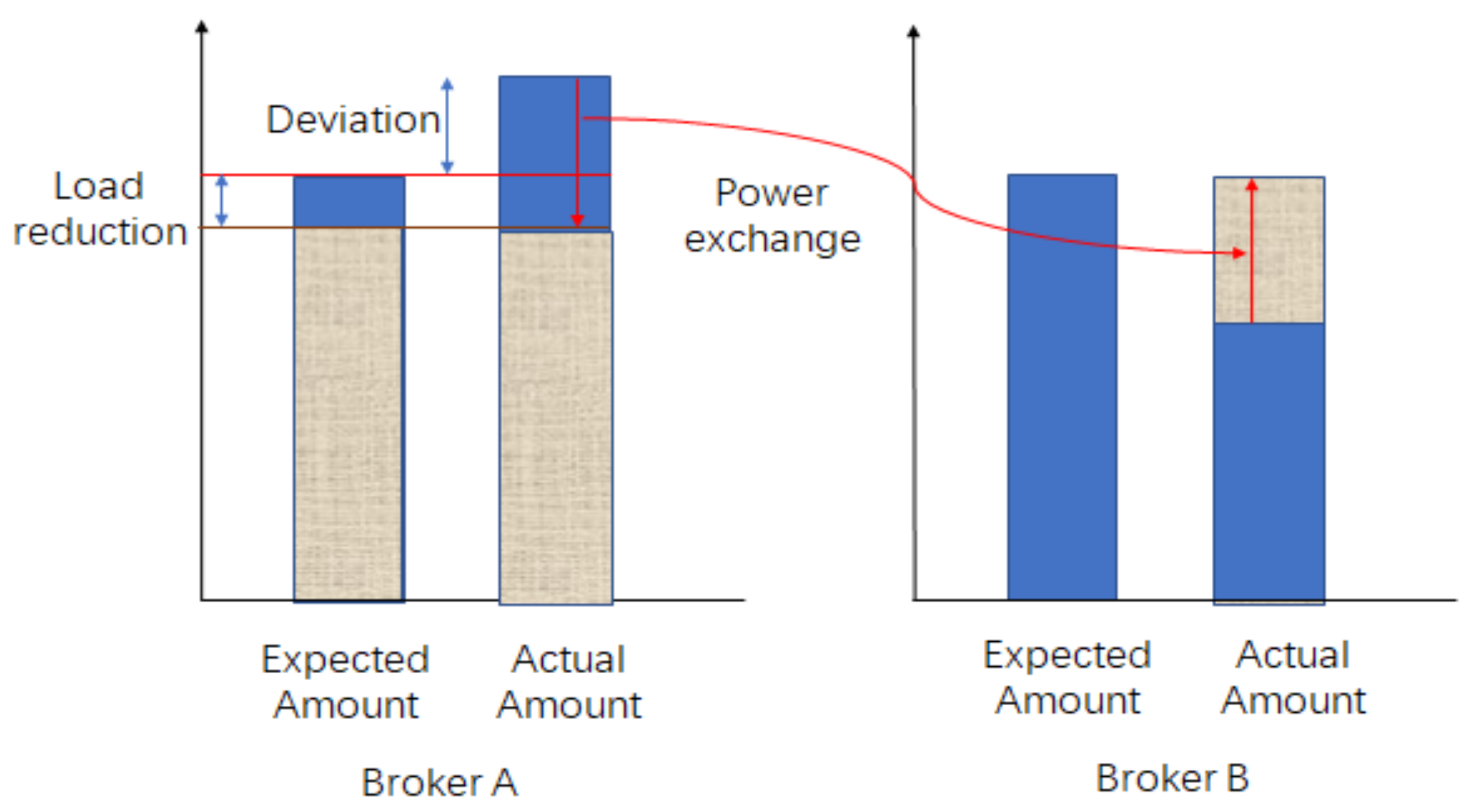
The constraints from Equations (16) to (20) are related to the power exchange strategy, where $u_{\mathit{ij},d,t,s}^{\mathrm{de}}$ is the state vector, while $u_{\mathit{ij},d,t,s}^{\mathrm{de}}=1$ means the power exchange occurs from area i to j in scenario sat time t in day d and $u_{\mathit{ij},d,t,s}^{\mathrm{de}}=0$ means it not happen. Equations (16) and (17) are the upper limit for power exchange amount. Equation (18) represents the direction of power exchange should be one-way rather than two-way. Equation (19) is the power balance equation when utilizing the power exchange strategy. Equation (20) means in every time period, the internal controllable elements amount within one area should not larger than the power purchase deviation. Otherwise, the power exchange strategy between areas is meaningless.

The last part is the robustness constraint of electricity price, as indicated below:

$$C_{d,t}^{\mathrm{rt}}=C_{d,t}^{\mathrm{da}}+\Delta C_{d,t}$$

(21)

$$C_{d,t}^{\mathrm{da}}=C_{d,t}^{\mathrm{da},\mathrm{p}}+{\alpha }_{d,t}^{\mathrm{da}}\left(C_{d,t,\max }^{\mathrm{da}}-C_{d,t}^{\mathrm{da},\mathrm{p}}\right)$$

(22)

$$0<={\alpha }_{d,t}^{\mathrm{da}}<=1$$

(23)

$${\displaystyle \sum _d{\displaystyle \sum _t{\alpha }_{d,t}^{\mathrm{da}}}}\le \Gamma$$

(24)

The relationship between the day-ahead and real-time market price is shown in Equation (21), and they are both stochastic. In comparison with day-ahead market price, the real-time market price is a little higher. The residual price $\Delta C_{d,t}$ is defined as the difference between them [20].

The constraints from Equations (22) to (24) are related to the robustness of power purchase price variables. In monthly optimization, the optimal power purchase decision is obtained based on the worst power purchase price (in general, the impact of higher day-ahead and real-time market prices on broker’s profit is tremendous), so when describing the fluctuation between the actual and forecast price, only the positive fluctuation is considered. The day-ahead market price $C_{d,t}^{\mathrm{da},\mathrm{p}}$ can be predicted from an ARIMA model [21]. In Equation (22), the actual price $C_{d,t}^{\mathrm{da}}$ is expressed as a linear function of the forecast value $C_{d,t}^{\mathrm{da},\mathrm{p}}$ and forecast error factor ${\alpha }_{d,t}^{\mathrm{da}}$ and this constraint represents the degree of fluctuation of the actual price relative to the predicted price. Equation (23) represents the upper and lower limit for the forecast error factor [22] ${\alpha }_{d,t}^{\mathrm{da}}$. Thus the actual day-ahead market price fluctuates between the maximum and forecast price. 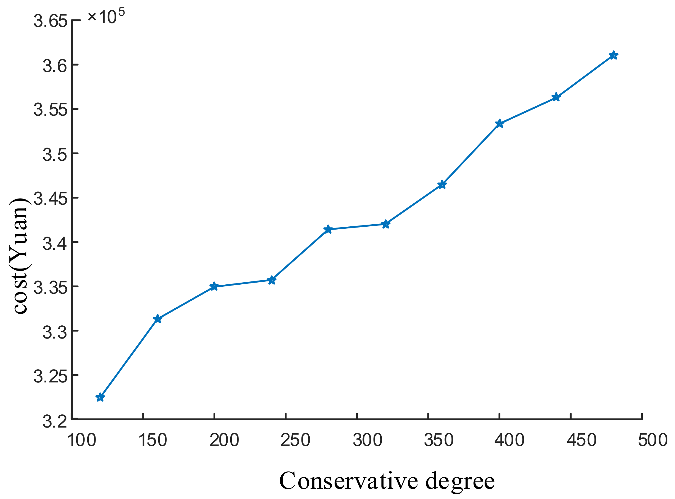In Equation (24), $\Gamma$ represent the conservative degree of the robust optimization problem, which means the worst positive price fluctuation that brokers could accept. $\Gamma$ could be set in range 0 to 720 because there are 720 time period in a month and forecast error factor ${\alpha }_{d,t}^{\mathrm{da}}$ could only fluctuates between 0–1 in a time period.

After day-ahead market clearing, brokers would prepare their dispatch schedules for controllable elements according to the result of monthly optimization, and the power exchange amount between areas could be derived post day-ahead optimization.

3.3. Post Day-Ahead Optimization Model of Areas

If the power purchase amount and cost in day-ahead market show an extreme mismatch with the forecast values from monthly optimization, the brokers would generally adjust the controllable elements dispatch schedules to eliminate the deviation between the actual and expected power purchase amount. Because the flexible loads have signed contracts with brokers in advance, changing their dispatch schedule inevitably affect the energy consumption behavior and, in turn, the satisfaction of users. By contrast, the dispatch schedule change for storage energy has a smaller impact. Thus, in order to correct this deviation, it is better to adjust the dispatch schedule of energy storage. In order to adapt to scenarios with different deviation, two strategies are proposed to solve this issue:

(1)

Executing the controllable elements dispatch schedule with monthly optimization. The objective function of post day-ahead optimization is shown in Equation (25). Since the controllable elements dispatch schedule and power purchase deviation occurred in the day-ahead market are all determined, the scenarios changes into s’, and $P_s$ is also removed which is the probability of scenario s. The net value $L_{d,s’,t,i}^{\mathrm{rt}}$ which equals to the load minus output of run-off hydro power station is the uncertain variable. The other constraints are similar with Equations (3) to (24):

$$\min {\displaystyle \sum _{s’}{\displaystyle \sum _i\left[{\displaystyle \sum _t{C}_i^{\mathrm{I}}{L}_{i,s’,d,t}^{\mathrm{I}}}+{\displaystyle \sum _{t_1\ne t_2}{C}_i^{\mathrm{Sh}}{L}_{i,s’,d,t_1,t_2}^{\mathrm{Sh}}}\right.}}+C_i^{\mathrm{Ec}}{L}_{i,s’,d,t}^{\mathrm{Ec}}+C_i^{\mathrm{Ed}}{L}_{i,s’,d,t}^{\mathrm{Ed}}+\left.{\displaystyle \sum _{j\ne i}{C}_{\mathit{ij}}^{\mathrm{Tr}}(L_{\mathit{ji},d,t}^{\mathrm{Tr}}+L_{\mathit{ij},d,t}^{\mathrm{Tr}})}+C_{d,t}^{\mathrm{rt}}{L}_{d,s’,t,i}^{\mathrm{rt}}\right]\Delta t$$

(25)

(2)

Adjusting the energy storage dispatch schedule. Therefore, the objective function of post day-ahead optimization is replaced by Equation (26), where the adjustment cost for energy storage is included; $U_{\mathrm{ESS},i}^{\mathrm{C}}$ is defined as adjusted status variable for energy storage. $U_{\mathrm{ESS},i}^{\mathrm{C}}=1$ means the energy storage of the area i is dispatched and $U_{\mathrm{ESS},i}^{\mathrm{C}}=0$ means it not dispatched:

$$\min \left\{{\displaystyle \sum _i{C}_{i,u}^{\mathrm{ESS}}{U}_{\mathrm{ESS},i}^{\mathrm{C}}}+{\displaystyle \sum _{s’}{\displaystyle \sum _i\left[{\displaystyle \sum _t{C}_i^{\mathrm{I}}{L}_{i,s’,d,t}^{\mathrm{I}}}+\right.}}\right.{\displaystyle \sum _{t_1\ne t_2}{C}_i^{\mathrm{Sh}}{L}_{i,s’,d,t_1,t_2}^{\mathrm{Sh}}}+C_i^{\mathrm{Ec}}{L}_{i,s’,d,t}^{\mathrm{Ec}}+C_i^{\mathrm{Ed}}{L}_{i,s’,d,t}^{\mathrm{Ed}}+\left.\left.{\displaystyle \sum _{j\ne i}{C}_{\mathit{ij}}^{\mathrm{Tr}}(L_{\mathit{ji},d,t}^{\mathrm{Tr}}+L_{\mathit{ij},d,t}^{\mathrm{Tr}})}+C_{d,t}^{\mathrm{rt}}{L}_{d,s’,t,i}^{\mathrm{rt}}\right]\right\}$$

(26)

In addition to the constraints (3) to (24), Equation (27) is the upper quantity limit for the adjusted energy storage:

$${\displaystyle \sum _i|U_{\mathrm{ESS},i}^{\mathrm{C}}-U_{i,d}^{\mathrm{ESS}}}|\le \lambda$$

(27)

where $U_{\mathrm{ESS},i}^{\mathrm{C}}$, $U_{i,d}^{\mathrm{ESS}}$ represent the adjusted and initial status for energy storage within area i; $\lambda$ is the upper limit.

In post day-ahead optimization, the areas need to clear some part of their dispatched controllable elements to eliminate internal deviation and exchange cost. Therefore, extra constraints and variables that suggest the relationship of the lender to borrower and controllable elements exchange amount need to be added in these two optimizations:

$$L_{\mathit{ji},d,t}^{\mathrm{Tr}}=L_{\mathit{ji},d,t}^{\mathrm{Tr},\mathrm{pd}}+{\displaystyle \sum _k{L}_{\mathit{ji},d,t}^{\mathrm{Tr},k}}$$

(28)

$$L_{\mathit{ij},d,t}^{\mathrm{Tr}}=L_{\mathit{ij},d,t}^{\mathrm{Tr},\mathrm{pd}}+{\displaystyle \sum _k{L}_{\mathit{ij},d,t}^{\mathrm{Tr},k}}$$

(29)

$$L_{i,d,t}^k=L_{i,s’,d,t}^{k,\mathrm{in}}+{\displaystyle \sum _j{L}_{\mathit{ij},d,t}^{\mathrm{Tr},k}}-{\displaystyle \sum _j{L}_{\mathit{ji},d,t}^{\mathrm{Tr},k}}$$

(30)

$$L_{\mathit{ji},d,t}^{\mathrm{Tr},\mathrm{pd}}-L_{\mathit{ij},d,t}^{\mathrm{Tr},\mathrm{pd}}+L_{i,d,t}^k=L_{i,s’,d,t}^{\mathrm{load}}-L_{i,d,t}^{\mathrm{da}}-L_{d,s’,t,i}^{\mathrm{rt}}$$

(31)

Equation (29) represents that the power exchange amount from area j to i is consist of $L_{\mathit{ji},d,t}^{\mathrm{Tr},\mathrm{pd}}$ and $L_{\mathit{ij},d,t}^{\mathrm{Tr},k}$, where $L_{\mathit{ji},d,t}^{\mathrm{Tr},\mathrm{pd}}$ is the purchased power exchange amount from area j to i; $L_{\mathit{ij},d,t}^{\mathrm{Tr},k}$ is the controllable element amount k that area i get from j through power exchange strategy. Equation (30) means that the controllable element k of area i is divided into the internal and exchange dispatch amount, $L_{i,s’,d,t}^{k,\mathrm{in}}$ is internal amount which is dispatched by area i to eliminate internal deviation. Equation (31) suggests that the leftover load which equals to total load minus day-ahead and real-time power purchase amount should be fully accommodated by the power exchange strategy.

4. Optimization Solving Algorithm

The monthly robust stochastic optimization model is a bi-level model, which isn’t easily solved directly. In order to simplify this model, it is necessary to convert the maximum solution into minimum according to the dual principle in the lower level.

First, by introducing the Equation (21) into (1), the lower level model which consists of the day-ahead and real-time market power purchase cost is separated from Equation (1) as Equation (32):

$$\begin{array}{l}{C}_{d,t}^{\mathrm{da}}{L}_{i,s,d,t}^{\mathrm{da}}+C_{d,t}^{\mathrm{rt}}{L}_{d,s,t,i}^{\mathrm{rt}}=C_{d,t}^{\mathrm{da}}(L_{i,s,d,t}^{\mathrm{da}}+L_{d,s,t,i}^{\mathrm{rt}})+\Delta C_{d,t}{L}_{d,s,t,i}^{\mathrm{rt}}=\left[C_{d,t}^{\mathrm{da},\mathrm{p}}\right.+\left.{\alpha }_{d,t}^{\mathrm{da}}\left(C_{d,t,\max }^{\mathrm{da}}-C_{d,t}^{\mathrm{da},\mathrm{p}}\right)\right](L_{i,s,d,t}^{\mathrm{da}}+L_{d,s,t,i}^{\mathrm{rt}})\\ +\Delta C_{d,t}{L}_{d,s,t,i}^{\mathrm{rt}}=\left(C_{d,t,\max }^{\mathrm{da}}-\right.\left.C_{d,t}^{\mathrm{da},p}\right)(L_{i,s,d,t}^{\mathrm{da}}+L_{d,s,t,i}^{\mathrm{rt}}){\alpha }_{d,t}^{\mathrm{da}}+(C_{d,t}^{\mathrm{da},\mathrm{p}}+\Delta C_{d,t})L_{d,s,t,i}^{\mathrm{rt}}+C_{d,t}^{\mathrm{da},\mathrm{p}}{L}_{i,s,d,t}^{\mathrm{da}}\end{array}$$

(32)

In order to concisely introduce the conversion process, the lower level model is briefly shown in Equation (33):

$${\max }_{\overline{\alpha }}f(\theta )\overline{\alpha }+g(\theta )$$

(33)

s.t.

$$\left[\begin{array}{c}A\\ B\end{array}\right]\overline{\alpha }<=\left[\begin{array}{c}C\\ \Gamma \end{array}\right]$$

(34)

where $\overline{\alpha }$ represents ${\alpha }_{d,t}^{\mathrm{da}}$ which means the column vector of the forecast error factor, $f(\theta )$ represents the part for $\left(C_{d,t,\max }^{\mathrm{da}}-\right.\left.C_{d,t}^{\mathrm{da},\mathrm{p}}\right)(L_{i,s,d,t}^{\mathrm{da}}+L_{d,s,t,i}^{\mathrm{rt}})$ which is a row vector; $g(\theta )$ stands for $(C_{d,t}^{\mathrm{da},\mathrm{p}}+\Delta C_{d,t})L_{d,s,t,i}^{\mathrm{rt}}+C_{d,t}^{\mathrm{da},\mathrm{p}}{L}_{i,s,d,t}^{\mathrm{da}}$ which is row vector, too. A is a unit diagonal array; B is a row vector where all elements are 1; C is a column vector where all elements are 1.

Then, since above lower level model are linear function of the variable ${\alpha }_{d,t}^{\mathrm{da}}$, according to dual principle, the lower level can be converted into the following models:

$$\min {\displaystyle \sum _t{\displaystyle \sum _d\left[\begin{array}{cc}{C}^T& \mathrm{\Gamma }\end{array}\right]\overline{\rho }+g(\theta )}}$$

(35)

s.t.

$$\left[\begin{array}{cc}A& B^T\end{array}\right]\overline{\rho }>={\left[f(\theta )\right]}^{\mathrm{T}}$$

(36)

$$\overline{\rho }>=\tilde{0}$$

(37)

where $\overline{\rho }$ is the dual variable of $\overline{\alpha }$. ${\left[f(\theta )\right]}^{\mathrm{T}}$ is the transposed matrix of $f(\theta )$. $\tilde{0}$ is the column vector whose all elements equals to 0.

The interruptible load constraints Equation (4) to Equation (7) include non-linear parts, according to [23], these non-linear parts can be linearized with adding the intra-day coupling constraint Equation (38):

$$\left\{\begin{array}{l}{\displaystyle \sum _{\mathsf{\tau }=t}^{\theta (T_{i,\mathrm{on}}^{\mathrm{I}},t)}{u}_{i,s,d,\mathsf{\tau }}^{\mathrm{I}}}\ge (u_{i,s,d,t}^{\mathrm{I}}-u_{i,s,d,t-1}^{\mathrm{I}})\eta (T_{i,\mathrm{on}}^{\mathrm{I}},t)+\epsilon (t-1){\theta }_{j,0}\\ {\displaystyle \sum _{\mathsf{\tau }=t}^{\theta (T_{i,\mathrm{off}}^{\mathrm{I}},t)}(1-u_{i,s,d,\mathsf{\tau }}^{\mathrm{I}})}\ge (u_{i,s,d,t-1}^{\mathrm{I}}-u_{i,s,d,t}^{\mathrm{I}})\eta (T_{i,\mathrm{off}}^{\mathrm{I}},t)+\epsilon (t-1){\eta }_{j,0}\end{array}\right.$$

(38)

where $\mathsf{\epsilon }(t-1)$ is an unit impact function, the $\theta \left(\omega ,t\right)$, $\eta (\omega ,t)$, ${\theta }_{j,0}$ and ${\eta }_{j,0}$ is calculated in Equation (39):

$$\left\{\begin{array}{c}\theta \left(\omega ,t\right)=\min \{t+\omega -1,T\}\\ \eta \left(\omega ,t\right)=\min \{\omega ,T-t+1\}\\ {\theta }_{j,0}=u_{i,s,d,1}^{\mathrm{I}}{u}_{i,s,d,0}^{\mathrm{I}}\max \{0,T_{i,\mathrm{on}}^{\mathrm{I}}-S_{\mathrm{on},i,s,d,t}^0\}\\ {\eta }_{j,0}=(1-u_{i,s,d,1}^{\mathrm{I}})(1-u_{i,s,d,0}^{\mathrm{I}})\max \{0,T_{i,\mathrm{off}}^{\mathrm{I}}-S_{\mathrm{off},i,s,d,t}^0\}\end{array}\right.$$

(39)

where $u_{i,0}^{\mathrm{I}}$, $S_{\mathrm{on},i}^0$ and $S_{\mathrm{off},i}^0$ represent the status variable for interruption load in final time period of last month, they are computed as follows:

$$S_{\mathrm{on},i,s,d,t}^0=\left\{\begin{array}{c}{S}_{\mathrm{on},i}^0\hspace{1em}d=1\\ u_{i,s,d-1,T}^{\mathrm{I}}\hspace{1em}d\ne 1\end{array}\right.$$

(40)

$$S_{\mathrm{off},i,s,d,t}^0=\left\{\begin{array}{c}{S}_{\mathrm{off},i}^0\hspace{1em}d=1\\ u_{i,s,d-1,T}^{\mathrm{I}}\hspace{1em}d\ne 1\end{array}\right.$$

(41)

$$u_{i,s,d,0}^{\mathrm{I}}=\left\{\begin{array}{c}{u}_{i,0}^{\mathrm{I}}\hspace{1em}d=1\\ u_{i,s,d-1,T}^{\mathrm{I}}\hspace{1em}d\ne 1\end{array}\right.$$

(42)

Finally, a single level model which constraints are all linear equations is derived. This single level model is a mix-integer linear programming problem, which could be solved by the Cplex solver as well as the post day-ahead model.

5. Case Study

5.1. Monthly Optimization Model of Areas

Alliances which include too many areas may cause a bad impact on the power market, so in the case study four areas {1, 2, 3, 4} are chosen, where the area a includes a pumped storage hydro power station while the areas {2, 3, 4} only include run-off hydro power stations. The monthly optimization model cycle is 24 h/30 d, the load and cost unit are kW and yuan/kWh, respectively. For the historical electricity price data, because the spot market has not been implemented in China, this paper refers to the electricity price data in the Nordic electricity market which is more perfect in the world and converts them through exchange rates. The charge and discharge cost for pumped storage hydro power is 0.008 yuan/kWh, the upper limit is 3 MWh. The other data are simulated by hydroelectric and load data from the areas of Sichuan, China. The curve of net load which is equal to the load minus output of uncontrollable hydro power station is shown in Figure 3. Figure 4 is the historical data of the day-ahead market price. The cost of the interruptible and transferrable loads is shown in Figure 5 and Figure 6. Other parameters are represented in

Table 1. Areas’ controllable elements parameters (kW).

Area	Upper Limit of IL	Lower Limit of IL	Upper Limit of TL between Two Time	Upper Limit of TL in a Time	Capacity for NS (kW)	Maximum Charge/Discharge (kW)
1	1.1%	3.1%	1.75%	4.05%	800	100
2	0.95%	3.05%	1.9%	4.1%	850	100
3	1%	2.8%	1.8%	3.8%	850	100
4	1.1%	2.9%	1.9%	4%	800	100

IL = interruptible load; TL = transferable load; NS = energy storage.

. The power exchange cost and daily controllable elements dispatch costs are proposed in

Table 2. Areas’ power exchange costs.

Borrow Lend	Area 1 (Yuan/kWh)	Area 2 (Yuan/kWh)	Area 3 (Yuan/kWh)	Area 4 (Yuan/kWh)
Area 1	/	0.0019	0.0029	0.0134
Area 2	0.0178	/	0.0146	0.0146
Area 3	0.0038	0.0174	/	0.0046
Area 4	0.0058	0.0104	0.0108	/

and

Table 3. Areas’ daily controllable elements dispatch costs.

Area	1	2	3	4
Interruptible load (Yuan/d)	138	205	127	136
Transferable load (Yuan/d)	137	194	126	174
Energy storage (Yuan/d)	181	212	193	139

.

According to the net load from different dates, the typical scenarios in the day-ahead market are obtained through the Monte Carlo sampling method and K-means clustering algorithm. If the scenarios are excessive, the speed of the solving process will slow down greatly. In order to ensure both speed and quality of solving process, 10 typical scenarios are chosen in this paper.

The monthly optimization can be finished by the Cplex solver in 5 h with 0.01% error accuracy. The probability of every scenario and the absolute value of all the power purchase deviation in one optimization cycle are shown in

Table 4. Power purchase deviation scenarios.

Scenario	1	2	3	4	5
Probability	0.1176	0.0955	0.11	0.0981	0.0996
Total deviation (kWh)	198,299	222,294	202,591	214,062	214,246
Scenario	6	7	8	9	10
Probability	0.0763	0.0998	0.0965	0.1029	0.1037
Total deviation (kWh)	236,755	212,380	215,851	211,144	211,552

.

The cost of all areas is 3.526 × 10⁵ yuan in the optimization results, and the dispatch dates of the controllable elements are also obtained. The dispatch dates in the first 7 days is given in

Table 5. Controllable elements dispatch date.

Day		1	2	3	4	5	6	7
Area 1	Interruptible load	1	0	0	0	0	1	0
	Transferrable load	1	0	1	1	0	1	1
	Energy storage	0	0	1	0	1	0	0
Area 2	Interruptible load	1	0	1	1	1	0	0
	Transferrable load	0	1	1	0	1	0	0
	Energy storage	1	0	0	0	0	0	0
Area 3	Interruptible load	1	0	1	1	0	1	0
	Transferrable load	0	1	0	0	0	1	0
	Energy storage	1	0	0	0	1	0	0
Area 4	Interruptible load	1	0	0	0	1	0	0
	Transferrable load	1	0	0	0	1	0	0
	Energy storage	0	1	1	1	0	0	1

, where 0 represents that this controllable element is not dispatched, while 1 means it is dispatched.

The controllable elements dispatch date of areas is related to the power purchase deviation, price, and controllable elements cost. As the dispatch dates in Table 5 show, with the forecast load, more types of controllable elements are dispatched when the areas have a heavy loads with bigger power purchase deviations.

According to the dispatch date, the times of any two types of the controllable elements dispatched within one area or between areas both can be obtained, which means the coordinative operation times for controllable elements. The coordination times are shown in Figure 7. Obviously, the coordination times of different types of controllable elements is more than the coordination times of similar types of controllable elements, because the same type of deviation can be handled similarly and different combinations are more effective and practical. The transferrable load is limited by its transfer time and energy storage is hindered by the charging and discharging process. By contrast, the cooperative operation of interruptible loads and energy storage is the best one, since it can be adjusted to eliminate different types of deviations at in any time period.

The conservative degree of robust variables means the maximum price fluctuation that the decision-maker would accept. Figure 8 shows all areas’ cost changes with the conservative degree, which suggests they are positively correlated. When controllable elements dispatch date changes, under the different scenarios, the controllable elements amount used to eliminate the deviation vary differently.

In contrast with three different types of schemes: (1) ignoring the controllable elements dispatch date; (2) ignoring the power exchange strategy; (3) ignoring both of them the results of every optimization scheme are shown in

Table 6. Comparison of different optimization schemes (Yuan).

Scheme	Scheme 1	Scheme 2	Scheme 3	Scheme 4
CS dispatch cost	5.89 × 104	3.68 × 104	5.90 × 104	1.97 × 104
Operation cost	3.40 × 105	3.78 × 105	3.97 × 105	3.33 × 105
Total cost	3.99 × 105	4.15 × 105	4.56 × 105	3.53 × 105

*CS = controllable element.

.

In Scheme 1, the controllable elements are all dispatched in a cycle. Although the power purchase cost is reduced greatly, the utilization of the controllable elements is not high, and the cost is still relatively high, the controllable elements need be dispatched every day. In Scheme 2, the cost is relatively high too, because there is no controllable elements exchange between areas. In Scheme 3, the operation cost is the highest. By contrast, the scheme in this paper has better performance on eliminating power purchase deviation due to the comprehensive consideration of controllable elements dispatch dates and a power exchange strategy.

Figure 9 shows that monthly optimization cost varies with capacity of every type of controllable element (pumped storage hydro power, energy storage device, interruptible loads, and transferrable loads). In the same deviation case, the capacity increase of any type controllable elements would reduce the power purchase deviation. However the whole optimization cost decrease trend would slow down because of the increase of controllable element capacity cost. Based on the preset monthly optimization results (intersection points in the graph), the changing trend of simulation results can be obtained by changing the capacity of various controllable elements and their influence on optimization by changing various controllable elements.

5.2. Post Day-Ahead Optimization of Areas

After the brokers bid in the power market, and the market clears, the price and power purchase deviation are both clear. According to the controllable elements dispatch date matrix U in the monthly optimization, the daily dispatch status is clear, too. The controllable elements dispatch amount in every period, power exchange amount, and controllable elements exchange amount can be obtained according to the results of monthly optimization, price after the clearing process, and power purchase deviation.

The power purchase deviation reduction percentages of power exchange, controllable elements dispatch and controllable elements exchange results are given in

Table 7. Power purchase deviation reduction by various strategy.

Day	Total Deviation (kWh)	Purchased Power Exchange	Internal CE Dispatch	CE Exchange Amount
1	5.843 × 103	35.72%	21.62%	14.53%
2	3.251 × 103	21.42%	25.87%	19.24%
3	5.128 × 103	28.53%	22.32%	15.21%
4	4.728 × 103	32.68%	12.78%	8.91%
5	4.252 × 103	47.91%	16.85%	17.39%

. According to Table 7, the deviation reduction ability of power exchange strategy is related to the total deviation. Because the controllable elements are limited by their own capacity and dispatch constraints, this has the ability to eliminate deviations as day 2 shows. The deviation reduction ability of controllable elements exchange is related to the leftover amount after areas have dispatched it to satisfy their own needs. In view of the results, the power exchange is the best while the controllable elements exchange is quite poor.

In Table 7, the deviation reduction percentage by controllable elements dispatch is small on day 4, because the deviation between the actual and expected power purchase amount occurred in the day-ahead market. The energy storage adjustment strategy is adopted to solve this problem. We contrast the optimization model 1 to 2 in Section 3.3, and the results are given in

Table 8. Impact of adjusting energy storage on deviation.

Scheme	Purchased Power Exchange	Internal CE Dispatch	CE Exchange	Area Dispatching Energy Storage	Total Operation Cost (Yuan)
1	32.68%	12.78%	8.91%	3	1.23 × 104
2	32.68%	16.32%	12.70%	3,4	1.14 × 104

.

In contrast with Scheme 1, Scheme 2 is more capable in adjusting energy storage dispatch plans and eliminating the expected deviation.

6. Conclusions

This paper proposes an innovative trading mode, where a power exchange strategy between multiple areas is adopted through an alliance of areas. Then the monthly robust stochastic optimization considering power market price and power purchase deviation is constructed to obtain controllable elements dispatch dates. After the power market clearing process, the controllable elements dispatch amount, controllable elements exchange amount, and power exchange amount are all obtained through the post day-ahead market optimization, which contains two different energy storage adjustment strategies. The conclusions of this paper are summarized as follows:

(1)

Power purchase deviations can be eliminated by the dispatch of controllable elements, and controllable elements exchange through the power exchange strategy. Deviations from different scenarios can be better eliminated by the combination of controllable elements.

(2)

The daily dispatch plan of controllable elements can be obtained by the monthly optimization, which can enhance its utilization and eliminate the power purchase deviations in some extent, to avoid resource waste situations. Two optimization models related to energy storage adjustment can be referenced by the area’s decision makers for different deviations situations.

(3)

The monthly optimization model for areas is a bi-level model which can be converted into one-phase model by the duality principle, and the non-linear constraints can be linearized as well. Finally, the mix-integer linear programming model is obtained, which can be efficiently and accurately solved by the Cplex solver. This paper offers a new choice for areas to solve the forward market optimization issue with a tiny time interval.

In further work, because intraday variables feature coupling constraints, the complex forward market optimization model need to be solved. Also, the time scale can be optimized by the descending dimension method to reduce the time of the optimization.

References

1. Ming, B.; Liu, P.; Cheng, L.; Zhou, Y.; Wang, X. Optimal daily generation scheduling of large hydro–photovoltaic hybrid power plants. Energy Convers. Manag. 2018, 171, 528–540. [Google Scholar] [CrossRef]
2. Hosseini, S.M.H.; Forouzbakhshb, F.; Rahimpoora, M. Determination of the optimal installation capacity of small hydro-power plants through the use of technical, economic and reliability indices. Energy Policy 2005, 33, 1948–1956. [Google Scholar] [CrossRef]
3. Yang, J.; Zhao, J.; Luo, F.; Wen, F.; Dong, Z.Y. Decision-Making for Electricity Retailers: A Brief Survey. IEEE Trans. Smart Grid 2018, 9, 4140–4153. [Google Scholar] [CrossRef]
4. Hatami, A.R.; Seifi, H.; Sheikh-El-Eslami, M.K. Optimal selling price and energy procurement strategies for a retailer in an electricity market. Elec. Power Syst. Res. 2009, 79, 246–254. [Google Scholar] [CrossRef]
5. Yang, J.; Zhao, J.; Wen, F.; Dong, Z.Y. A Framework of Customizing Electricity Retail Prices. IEEE Trans. Power Syst. 2018, 33, 2415–2428. [Google Scholar] [CrossRef]
6. Do Prado, J.C.; Qiao., W. Stochastic Decision-Making Model for an Electricity Retailer with Intermittent Renewable Energy and Short-term Demand Response. IEEE Trans. Smart Grid 2018. [Google Scholar] [CrossRef]
7. Mahmoudi, N.; Eghbal, M.; Saha, T.K. Employing demand response in energy procurement plans of electricity retailers. Int. J. Electr. Power Energy Syst. 2014, 63, 455–460. [Google Scholar] [CrossRef]
8. Song, M.; Amelin, M. Purchase bidding strategy for a retailer with flexible demands in day-ahead electricity market. IEEE Trans. Power Syst. 2017, 32, 1839–1850. [Google Scholar] [CrossRef]
9. Wu, H.; Shahidehpour, M.; Alabdulwahab, A.; Abusorrah, A. Demand Response Exchange in the Stochastic Day-Ahead Scheduling With Variable Renewable Generation. IEEE Trans. Sustain. Energy 2015, 6, 516–525. [Google Scholar] [CrossRef]
10. Shafie-khah, M.; Heydarian-Fourushani, E.; Golshan, M.E.H.; Moghaddam, M.P.; Sheikh-El-Eslami, M.K.; Catalão, J.P.S. Strategic Offering for a Price-Maker Wind Power Producer in Oligopoly Markets considering Demand Response Exchange. IEEE Trans. Ind. Inform. 2015, 11, 1542–1553. [Google Scholar] [CrossRef]
11. Tavakoli, A.; Negnevitsky, M.; Nguyen, D.T.; Muttaqi, K.M. Energy Exchange between Electric Vehicle Load and Wind Generating Utilities. IEEE Trans. Power Systems 2016, 31, 1248–1258. [Google Scholar] [CrossRef]
12. Yangfang, Y.; Jichun, L. Two-stage Decision-making Method of Retailers Considering Power Transfer Strategy. Autom. Electric Power Syst. 2017, 24, 120–128. [Google Scholar]
13. Zheng, O.P.; Wang, J.; Liu, A.L. Stochastic Optimization for Unit Commitment—A Review. IEEE Trans. Power Syst. 2015, 30, 1913–1924. [Google Scholar] [CrossRef]
14. Kazempour, S.J.; Conejo, A.J.; Ruiz, C. Strategic Bidding for a Large Consumer. IEEE Trans. Power Syst. 2016, 30, 848–856. [Google Scholar] [CrossRef]
15. Siahkali, H.; Vakilian, M. Stochastic unit commitment of wind farms integrated in power system. Electr. Power Syst. Res. 2010, 80, 1006–1017. [Google Scholar] [CrossRef]
16. Nojavan, S.; Zare, K.; Mohammadi-Ivatloo, B. Robust bidding and offering strategies of electricity retailer under multi-tariff pricing. Energy Econ. 2017, 68, 359–372. [Google Scholar] [CrossRef]
17. Murphy, C.; Soroudi, A.; Keane, A. Information Gap Decision Theory-Based Congestion and Voltage Management in the Presence of Uncertain Wind Power. IEEE Trans. Sustain. Energy 2016, 7, 841–849. [Google Scholar] [CrossRef]
18. Golmohamadi, H.; Keypour, R. A bi-level robust optimization model to determine retail electricity price in presence of a significant number of invisible solar sites. Sustain. Energy Grids Netw. 2018, 13, 93–111. [Google Scholar] [CrossRef]
19. Chen, H.C. Optimum capacity determination of stand-alone hybrid generation system considering cost and reliability. Appl. Energy 2013, 103, 155–164. [Google Scholar] [CrossRef]
20. Baringo, A.; Baringo, L. A Stochastic Adaptive Robust Optimization Approach for the Offering Strategy of a Virtual Power Plant. IEEE Trans. Power Syst. 2017, 32, 3492–3504. [Google Scholar] [CrossRef]
21. Conejo, A.J.; Contreras, J.; Espínola, R.; Plazas, M.A. Forecasting electricity prices for a day-ahead pool-based electric energy market. Int. J. Forecast. 2005, 21, 435–462. [Google Scholar] [CrossRef]
22. Xudong, Z.; Haojing, W.; Geng, W.U.; Ming, Z.; Xuan, Z. Robust power-loss cost optimization model considering price uncertainty for active distribution network. Available online: http://www.en.cnki.com.cn/Article_en/CJFDTotal-DLZS201709018.htm (accessed on 21 March 2019).
23. Madrigal, M.; Quintana, A.D. Semidefinite programming relaxations for {0,1}-power dispatch problems. In Proceedings of the 1999 IEEE Power Engineering Society Summer Meeting, Edmonton, AB, Canada, 18–22 July 1999. [Google Scholar]
Figure 1. Power exchange from broker A with positive deviation to broker B with negative deviation.
Energies 12 01160 g001
Figure 2. The monthly optimization result. IL = interruptible load; TL = transferable load; NS = energy storage.
Energies 12 01160 g002
Figure 3. Areas’ forecast net load curve for one day.
Energies 12 01160 g003
Figure 4. Historical day-ahead electricity price data.
Energies 12 01160 g004
Figure 5. Areas’ interruptible load costs.
Energies 12 01160 g005
Figure 6. Areas’ transferable load costs.
Energies 12 01160 g006
Figure 7. Controllable elements cooperative operation times.
Energies 12 01160 g007
Figure 8. The influence of robust conservative degree on cost.
Energies 12 01160 g008
Figure 9. Influence of controllable elements capacity on optimization cost.
Energies 12 01160 g009