Article

MPC with Constant Switching Frequency for Inverter-Based Distributed Generations in Microgrid Using Gradient Descent

Department of Electrical Engineering, Incheon National University, Songdo-dong, 119 Academy-ro, Yeonsu-gu, Incheon 22012, Korea
*
Author to whom correspondence should be addressed.
Energies 2019, 12(6), 1156; https://doi.org/10.3390/en12061156
Submission received: 13 February 2019 / Revised: 21 March 2019 / Accepted: 22 March 2019 / Published: 25 March 2019
(This article belongs to the Special Issue Control in Power Electronics)

Abstract

:
Variable switching frequency in the finite control set model predictive control (FCS-MPC) method causes a negative impact on the converter efficiency and the design of the output filters. Several studies have addressed the problem, but they are either complicated or require heavy computation. This study proposes a new model predictive control (MPC) method with constant switching frequency, which is simple to implement and needs only a small computation time. The proposed MPC method is based on the gradient descent (GD) method to find the optimal voltage vector. Since the cost function of the MPC method is represented in the strongly convex function, the optimal voltage vector could be found quickly by using the GD method, which reduces the computation time of the MPC method. The design of the proposed MPC method based on GD (GD-MPC) is shown in this study. The feasibility of the proposed GD-MPC is evaluated in the real-time simulation using OPAL-RT technologies. The performance of the proposed method in the case of single inverter operation or parallel inverter operation is shown. A comparison study on the proposed GD-MPC and the MPC with the concept of the virtual state vector (VSV-MPC) is presented to demonstrate the effectiveness of the proposed predictive control. Real-time simulation results show that the proposed GD-MPC method performs better with a low total harmonic distortion (THD) value of output current and short computation time, compared to the VSV-MPC method.

1. Introduction

Finite control set model predictive control (FCS-MPC) has been widely used for controlling the power converters in the microgrid (MG) system. Based on the discrete-time model of the converter system with the finite number of switching states, the FCS-MPC technique predicts all of the future behaviors of the controlled variables. A cost function that considers the error between the controlled variable and the desired reference is defined. The control action that minimizes the cost function is given directly for the power converter without a modulator [1,2,3]. The cost function of the FCS-MPC method is flexible; it is easy to include system constraints, nonlinearities, and multi-variable control objectives [4,5,6]. With the intuitive concept, the FCS-MPC technique has been used in various fields of applications [1,7,8,9].
The absence of the modulator makes FCS-MPC attractive for the complex converter topologies. However, the variable switching frequency caused by the lack of a modulator is the major disadvantage of the FCS-MPC technique. Various negative impacts of the variable switching frequency on the control performance of the power converter have been reported, such as difficulty in the design of filters, undesired losses in the semiconductor, and reduced power quality [10,11,12]. This problem has been addressed recently in various studies. Modulated model predictive control (M2PC) has been adopted for various power converters such as front-end rectifiers, active filters, matrix converters [13,14,15,16,17]. In the M2PC technique, several cost functions for each specific sector have been identified as needing to be evaluated in every sampling time, which results in an increase of computation time. An improved M2PC technique for the three-phase inverter was proposed in [18]. In contrast to the conventional MPC technique where the cost function is based on the controlled variables such as filter voltage or current, the improved M2PC method used the cost function with the inverter voltage vector. As a result, the number of sectors involved in the calculation of M2PC is reduced from six to one. Although this solution could significantly reduce the calculation, the execution time of the improved M2PC was reduced by 30% compared to the conventional M2PC, and it is still higher than the conventional MPC. The frequency weighted predictive control is proposed in [19,20]; this model achieves a fixed switching frequency by designing a narrow band-stop filter or a low-pass filter. Although the spectrum of the load current could be manipulated, the complicated design of the band-stop filler and the complexities of predictive control are the main limitations of this technique. In [21], a virtual system simulator (VSS) was used as an auxiliary control to calculate the number of sampling points based on the simulated waveforms and their harmonic spectra. The use of VSS in addition to the conventional MPC algorithm increased the complexity of the predictive algorithm and the computational burden. Since the switching frequency of the converter is dependent on the switching period, the predictive control based on the regulation of the switching period could provide constant switching frequency [22,23]. Another interesting method to improve the FCS-MPC with constant switching frequency is to use the virtual state vectors (VSVs) [11,12,13,14,15,16,17,18,19,20,21,22,23,24]. Instead of evaluating the cost function with the real number of state vectors, additional virtual state vectors are proposed to be evaluated. The optimal duty cycle or the control input could be found based on the real and virtual state vectors. Implementing this method in the digital control platform is straightforward. The control performance could be improved by increasing the number of virtual state vectors. However, the large number of calculations and more powerful control platform are the limitations of this technique. To overcome these problems, many studies have proposed methods to decrease the computational cost of the MPC [24,25,26]. In [25], the computational burden was reduced by equivalent transformation and specialized sector distribution. However, this strategy could not improve the steady-state or dynamic performance of the converters. The finite control set model predictive current control (FCS-MPCC) strategy was proposed for a five-phase inverter by the 11 reconstructed virtual voltage vectors [24]. However, this control strategy can only be used in the five-phase inverter.
In this study, a new MPC with constant switching frequency based on gradient descent (GD-MPC) is proposed to overcome the problem. Similar to the conventional FCS-MPC technique, the cost function that considers both controlled variables and the desired references is defined first. Then, the voltage vector that optimizes the predefined cost function is found by the gradient descent method. Since the cost function of the FCS-MPC could be defined as the strongly convex function, the convergence speed of GD could be improved significantly, which results in the reduction of computational burden. The constant switching frequency is achieved by adding the modulator to the MPC.
The feasibilities of the proposed MPC technique is evaluated in the real-time simulator using OPAL-RT technologies. Several simulation scenarios are carried out to show the feasibility of the proposed method, such as load change, uncertainties in system variables, and nonlinear load condition. A comparison study of the proposed method with the proposed MPC based on virtual state vector in [11] (VSV-MPC) is presented to show the effectiveness of the proposed controller. A tested MG system with two inverter-based distributed generations is considered in this study to show the feasibility of the proposed method in the condition of power sharing among multiple inverters.
The remaining of this study is arranged as follows: the discrete-time model of the converter and the design VSV-MPC method is shown in Section 2. The proposed GD-MPC method is presented in Section 3. The real-time simulation results are described in Section 4. Finally, Section 5 summarizes the main conclusion of this study.

2. Predictive Voltage Control with Constant Switching Frequency based on Virtual State Vector

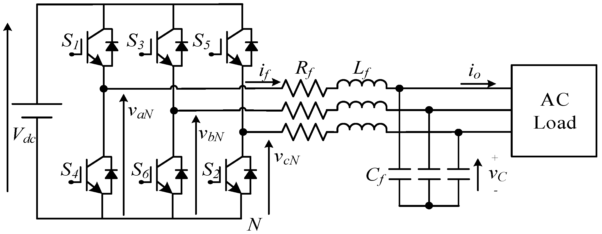
2.1. Conventional Predictive Voltage Control

A three-phase two-level voltage sources converter (VSC), which consists of three legs and an inductance and capacitor (LC) filter, is shown in Figure 1. There are two switches in a leg with two possible switching states. The combination of three legs creates eight different possible switching states, as given by Equation (1):
v t = 2 3 V d c e j ( n 1 ) ( π / 3 ) ( n = 1 , , 6 )
where V d c is the voltage of the direct current (DC) source.
The switching states of different combinations of voltage vectors can be expressed by: 000, 100, 110, 010, 011, 001, 101, and 111. The state-space model of the VSC, including an LC filter, can be written as:
d x d t = A x + B 1 v t + B 2 i o
x = [ i f v C ] , A = [ R f L f 1 L f 1 C f 0 ] , B 1 = [ 1 L f 0 ] , B 2 = [ 0 1 C f ]
where i f   and   v C are measured variables; v t can be calculated using Equation (1).
According to the method with the sampling time ( T s ), the discrete-time model of the VSC can be obtained from Equation (2), as follows:
x ( k + 1 ) = A d x ( k ) + B 1 d v t ( k ) + B 2 d i o ( k )
where A d = e A T s , B 1 d = 0 T s e A τ B 1 d τ , B 2 d = 0 T s e A τ B 2 d τ .
The predictive voltage of the capacitor can be calculated using Equation (3):
v C ( k + 1 ) = v C ( k ) + T s C f ( i f ( k ) i o ( k ) )
In the conventional predictive voltage control, the cost function can be expressed as:
J = ( v * C , α v C , α ( k + 1 ) ) 2 + ( v * C , β v C , β ( k + 1 ) ) 2
where v C , α ( k + 1 )   and   v C , β ( k + 1 ) are the real and imaginary parts of the predictive voltage of capacitor; and v * C , α   and   v * C , β are the real and imaginary parts of the reference.
By using Equation (5), the optimal voltage vector can be found to minimize the error between the reference and the predictive voltage of the capacitor.

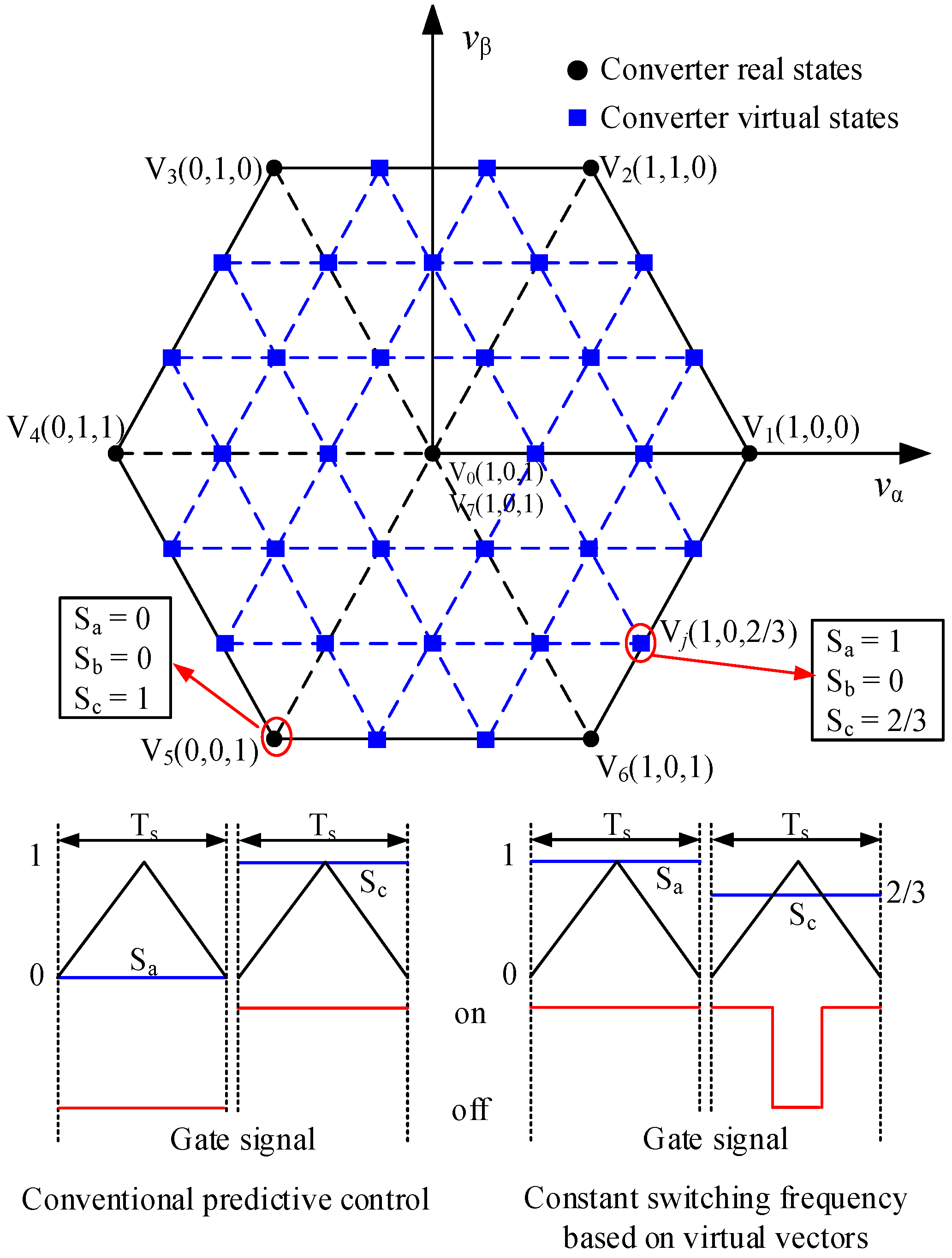
2.2. Predictive Voltage Control with Constant Switching Frequency Based on Virtual Vector

Conventional predictive voltage control considers the eight voltage vectors to predict the system response and evaluate the cost function. However, this method leads to variable switching frequency, and needs a high sampling time ( T s ) to maintain high performance. In order to overcome the problem of variable switching frequency, the predictive control with constant switching frequency using virtual vectors was proposed in [11]. The idea behind this control technique is to use additional virtual voltage vectors to evaluate the cost function. The optimal voltage vector including the virtual voltage vector is used to find the optimal control region. Then, the discrete space vector modulation (SVM) is used to generate the pulse signals for the power semiconductor. The virtual vectors can be obtained as a linear combination of real vectors ( v r e a l ) as follows:
v v i r = j = 1 , 2 , 3 t j , V j r e a l t 1 + t 2 + t 3 = T s w V j r e a l { V 0 , V 1 , , V 7 }
where T s w is the switching time. As the number of virtual vectors increases, the performance of the VSC is improved. Figure 2 shows eight real state vectors and 30 virtual state vectors.

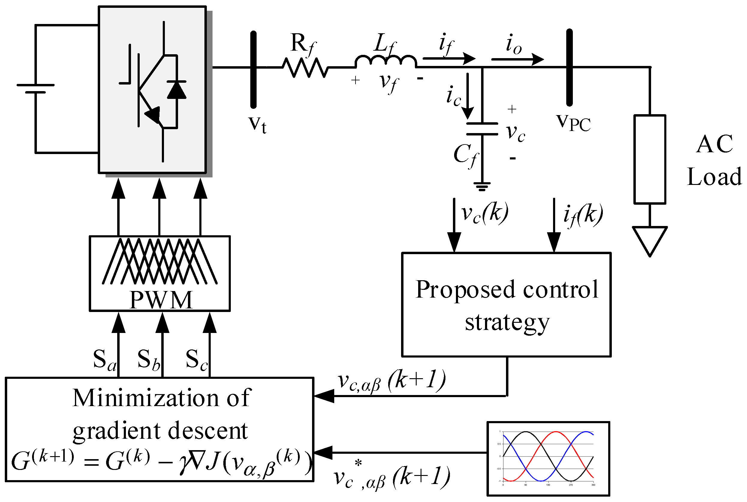
3. Proposed Predictive Voltage Control

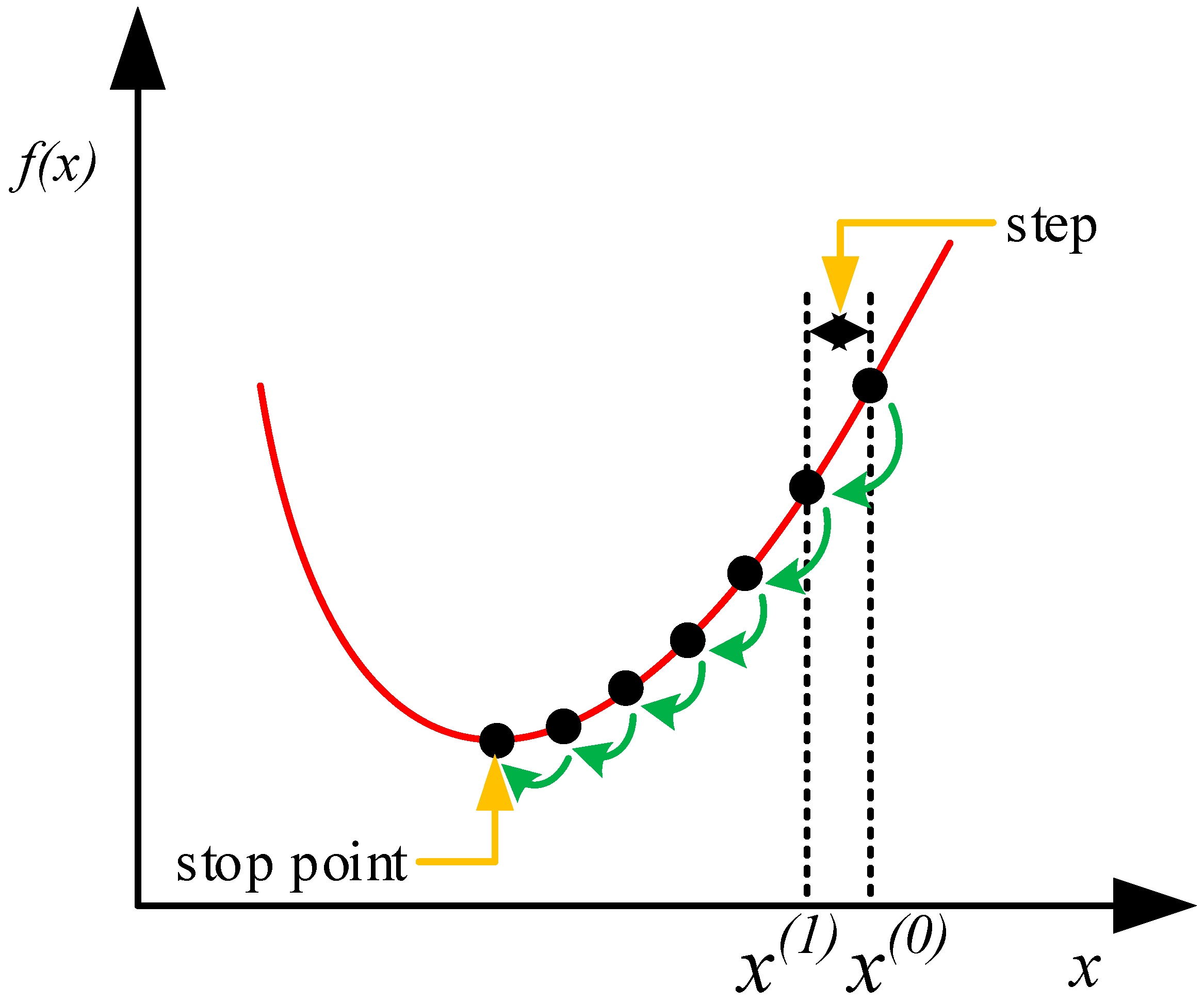
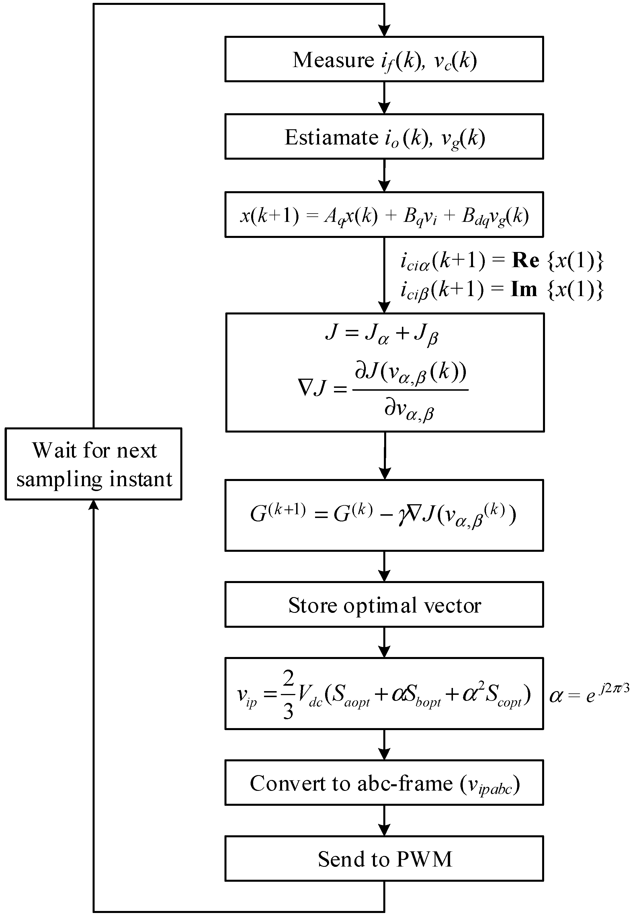
3.1. Gradient Descent

The gradient descent method, which is used for finding the minimum value of a convex function, is straightforward. There are two components to search for a stationary point: (i) the direction and (ii) the step size. It can be explained that this method typically starts at an arbitrary point ( x ( 0 ) ) and then at every step ( k ) iteratively moves in the direction of Δ x ( k ) by step size γ to the next point [27]:
x ( k + 1 ) = x ( k ) + γ Δ x ( k )
In gradient descent, the search direction is the negative slope at that point, i.e., Δ x = f ( x ) . Thus, iterative searches of gradient descents can be explained through the following recursive rules [27]:
x ( k + 1 ) = x ( k ) γ f ( x ( k ) )
where γ is the learning rate.
Algorithm 1 Gradient descent
Energies 12 01156 i001

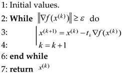
3.2. Proposed Predictive Control Strategy Based on Gradient Descent

The discrete-time model (Figure 2, Figure 3 and Figure 4) is used for prediction in the proposed GD-MPC method. Firstly, the cost function can be written in terms of v α ( k )   and   v β ( k ) as follows:
J = J α + J β { J α = ( i f α r e f ( i f α + ( T s v α ( k ) L f ) ( T s e α ( k ) L f ) ) ) 2 J β = ( i f β r e f ( i f β + ( T s v β ( k ) L f ) ( T s e β ( k ) L f ) ) ) 2
By using the gradient descent method to optimize the cost function J, the optimal voltage vector could be found. In order to find the minimal value of the cost function, the gradient of each cost function should be zero:
{ J α ( v α ) v α = 0 J β ( v β ) v β = 0
The gradient of cost function ( J = J α + J β ) results in:
J ( v α ) = 2 T s L f { i f α r e f ( i f α + ( T s v α ( k ) L f ) ( T s e α ( k ) L f ) ) } J ( v β ) = 2 T s L f { i f β r e f ( i f β + ( T s v β ( k ) L f ) ( T s e β ( k ) L f ) ) }
The gradient descent-based predictive control strategy (GD-MPC) iteratively updates function G in Equation (12) using the available voltage vector ( v α , v β ) until it reaches the stationary point corresponding (Figure 3) to the minimum value of the cost function:
G ( k + 1 ) = G ( k ) γ J ( v α , β ( k ) )
where k denotes the time instant, and γ is the learning rate of the gradient descent algorithm.
The overall control diagram of the proposed GD-MPC is shown in Figure 4, and Figure 5 shows the control algorithm of the GD-MPC method. The optimal voltage vector for the next sampling instant is found by the gradient descent. Pulse width modulation (PWM) is used to generate the pulse signals for the power converter based on the optimal voltage vector.

4. Simulation Results

The feasibility of the proposed MPC method is validated by real-time simulation using OPAL-RT technologies. The parameters of the converter and simulation are shown in Table 1. The impact of gradient descent on the control performance of the proposed MPC is presented. A comparison study on the proposed MPC and the MPC with a virtual state vector is presented in this section to show the effectiveness of the proposed method.

4.1. Single Converter Operation

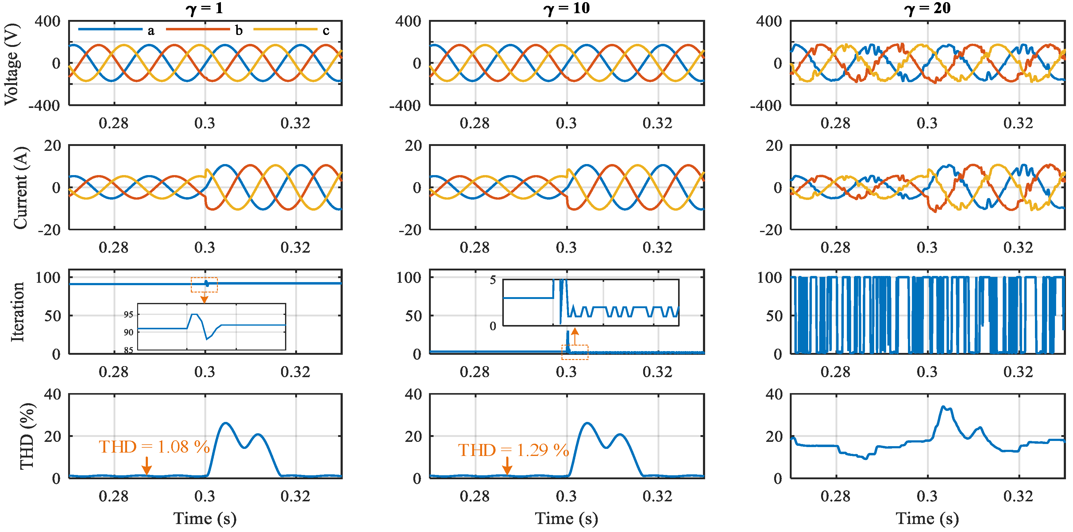
4.1.1. Effect of Learning Rate

Three cases are carried out to show the effect of the learning rate γ on the control performance of the converter system, which are γ = 1, γ = 10, and γ = 20. The real-time simulation results are shown in Figure 6. It is assumed that the load is increased at 0.3 s, and the root mean square (RMS) load voltage is 220 V. It can be seen that the proposed MPC with gradient descent is stably operated when the load is changed. In three cases, the inverter current is increased quickly to compensate for the load change.
It is observed that the learning rate γ has a significant impact on the computation of the proposed MPC method, as shown in the iteration in Figure 6. In case 1, which has a relatively small learning rate (γ = 1), the optimal voltage vector is found after 92 iterations. In case 2, in which γ is equal to 10, it takes only three iterations to find the optimal voltage vector; this is even smaller than the conventional MPC method, which takes seven iterations to obtain the optimal voltage vector. When the load current is increased, it takes only one or two iterations to obtain the optimal voltage vector. A significant computation time could be reduced by the proposed MPC method. However, if the learning rate γ is too large, the optimal voltage vector cannot be found within the maximum amount of iterations. This has a negative impact on the control performance of the converter system as shown in case 3, which has a γ value equal to 20.
It can be seen that the converter with a smaller learning rate value shows better performance. It can be seen in the THD comparison in Figure 6 that the value of THD in case 1 is the smallest, with a value of 1.08 %. The increase of learning rate could reduce the computation burden but increase the THD of the output current. However, the THD value of the output current is still small (THD = 1.29% in case 2).
The design of the proposed MPC method is based on the discrete-time model of the converter, in which the converter parameters such as L and C are assumed to be unchanged. However, the LC parameters could be changed by the operating condition of the converters, which might have a negative impact on the control performance of the MPC method. In this paper, it is assumed that the filter inductor L is changed, and its effect on the control performance is evaluated.

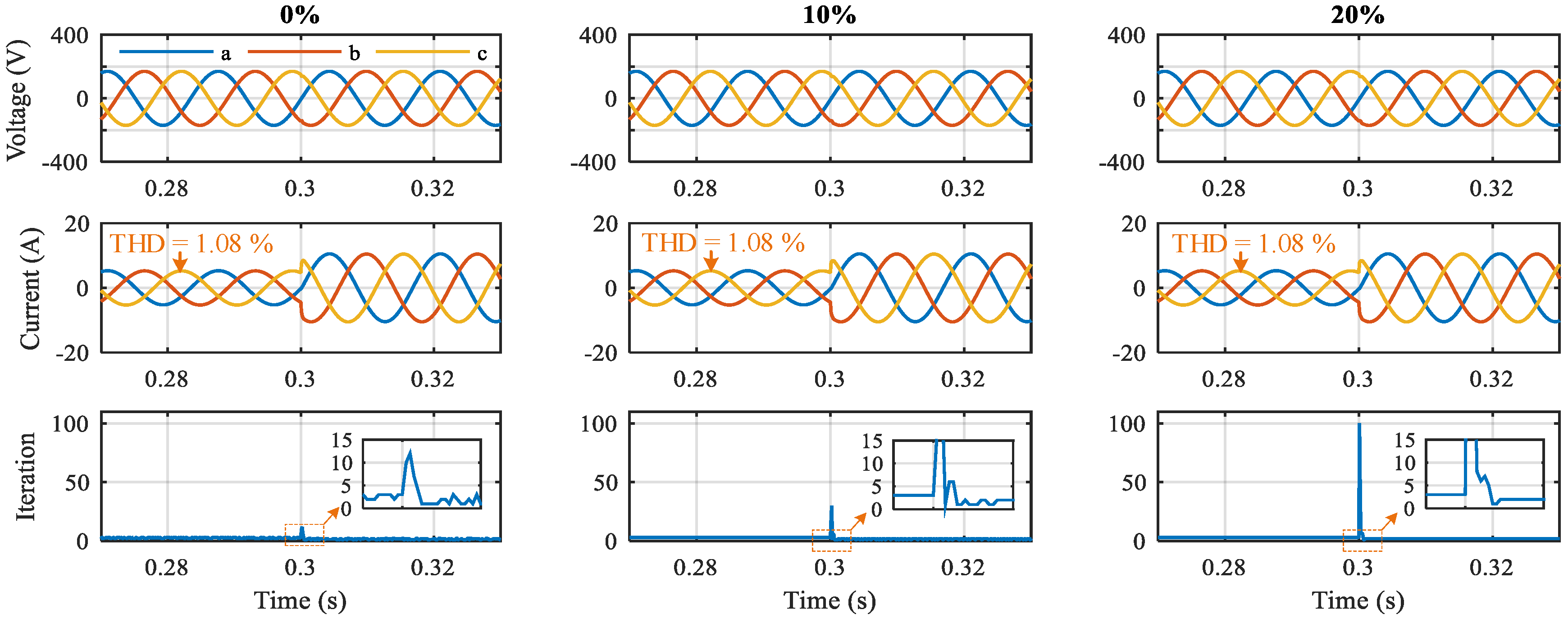
4.1.2. Effect of Uncertain Parameter

The MPC strategy is based on the model of the converter system to predict the future behavior of the controlled variable and find the optimal action based on the predicted variables. Thus, the change of converter parameters has an impact on the control performance of the MPC method. This section presents the effect of the uncertain parameter on the control performance of the proposed MPC method.
There are three cases are considered in this section, which are the original filter inductor L, a 10% change of L, and a 20% change of L. The real-time simulation results of three cases are shown in Figure 7. At 3 s, the load is increased, which results in an increase of inverter output current. It can be seen that the proposed MPC method is robust regarding the change of filter inductor. The output voltage and current of the converter are high qualities. There is an impact of the uncertain parameter on the control performance of the proposed method. It takes more iterations to find the optimal voltage vector when the filter inductor is changed. It can be seen that in the case of the original value of L, the maximum iteration to find the optimal voltage vector is 12 at the load changing. However, in the case of a 10% change in the L value, the maximal iteration is 30, whereas it is 100 in the case of a 20% change. However, the overall performance of the proposed method is stable in this scenario.

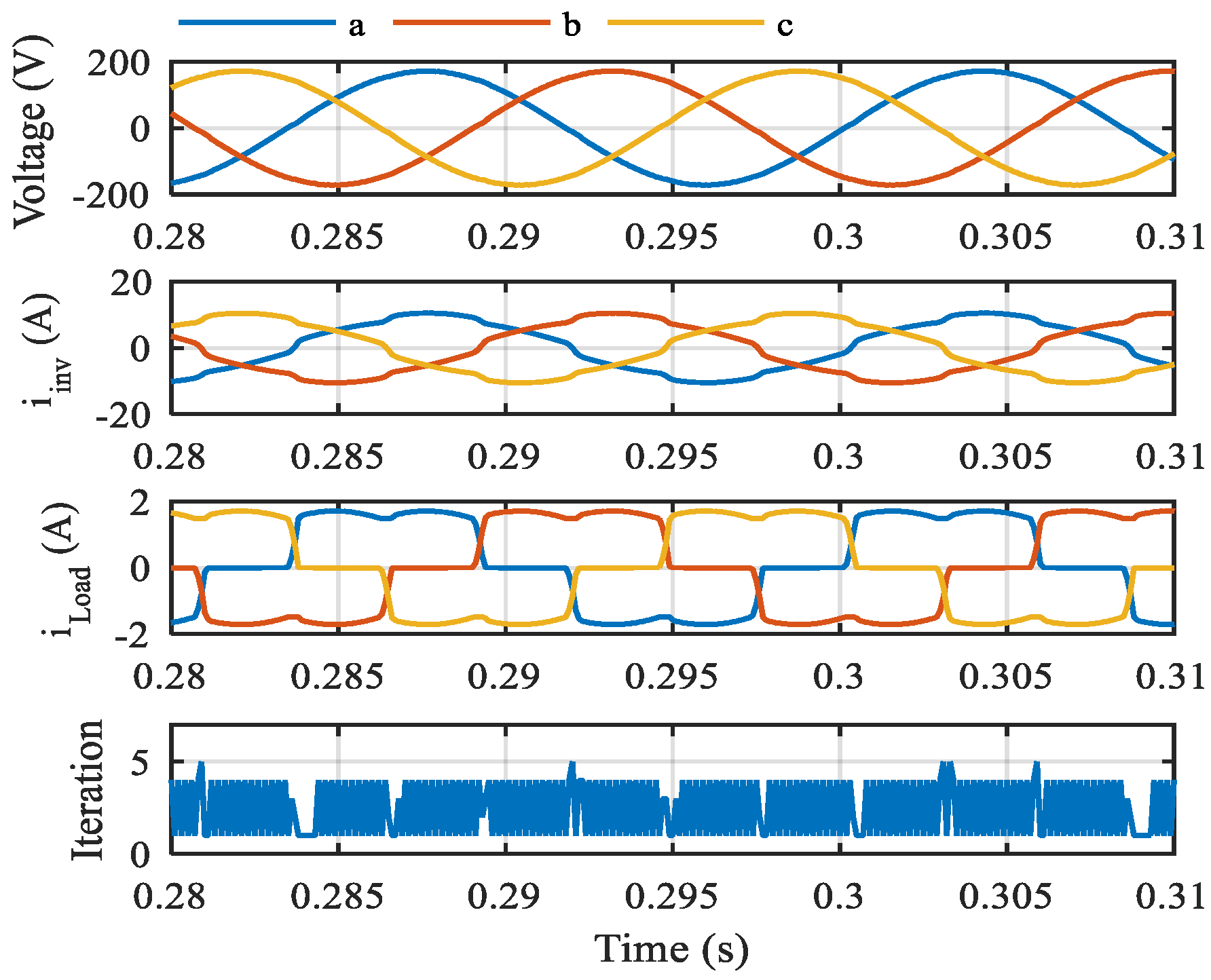
4.1.3. Nonlinear Load Condition

Figure 8 shows the control performance of the proposed MPC method in the nonlinear load condition. The diode bridge rectifier is used as a nonlinear load in this study. It can be observed that the output voltage is still sinusoidal, although the load current is highly distorted. The nonlinear load has a slight impact on the iteration of the proposed method. However, the maximum iteration is only five in this condition. Generally, the proposed MPC method is operated stably in this condition.

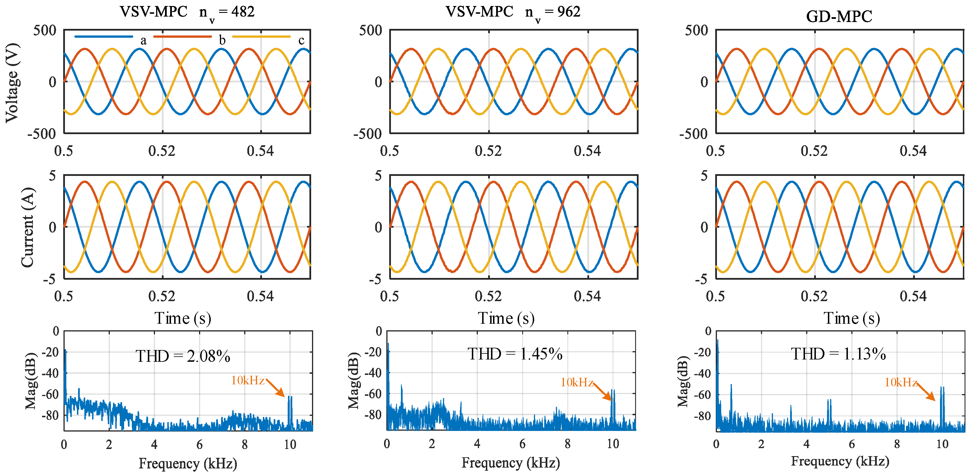
4.2. A Comparison Study

A comparison study on the proposed GD-MPC and the VSV-MPC in [11] is presented in this section. In the VSV-MPC method, there are two cases with a different number of virtual state vectors are carried out, which are 482 and 962 virtual state vectors.

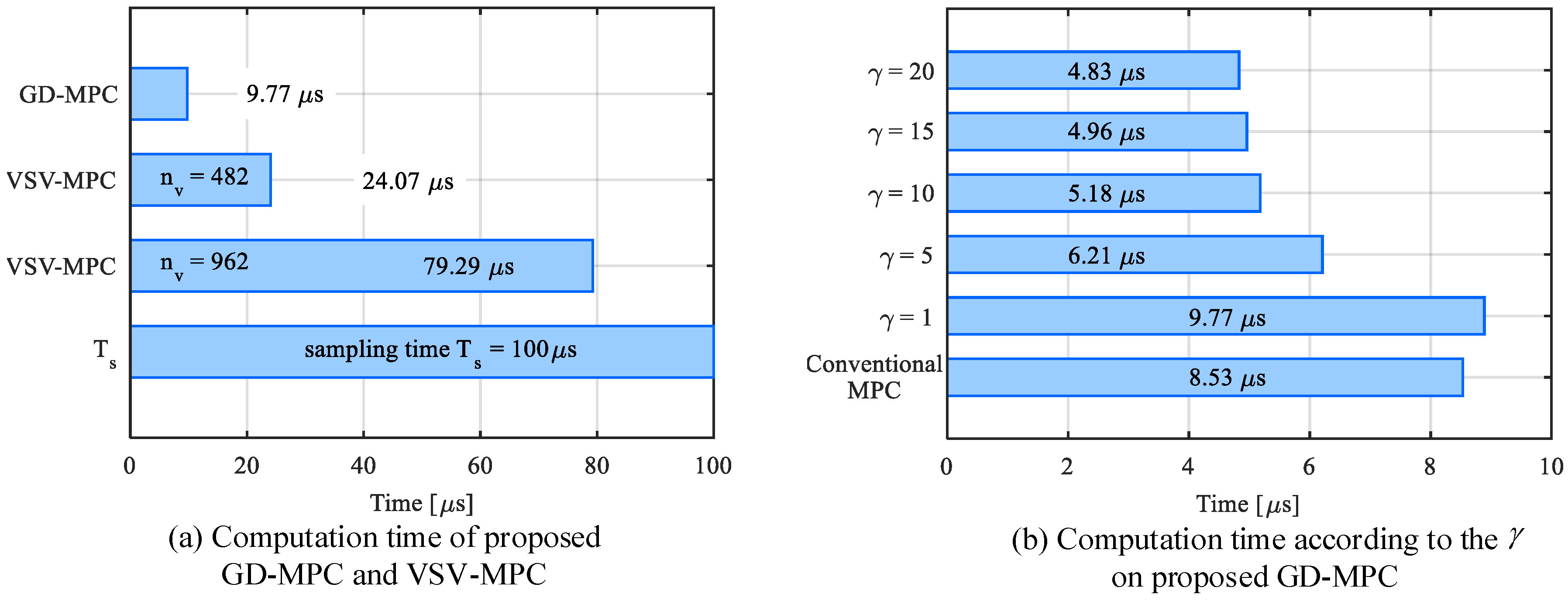
4.2.1. Computation Time

Figure 9 shows the comparison of the computation time of the proposed GD-MPC and other MPC techniques such as VSV-MPC and conventional MPC. It can be seen in Figure 9a that the proposed GD-MPC method could significantly reduce the computation time compared to the VSV-MPC method. The execution time of the GD-MPC is 9.77 μs, whereas it is 24.7 μs or 79.29 μs in the cases with the VSV-MPC method. The execution time of the proposed GD-MPC method is much smaller than that of the VSV-MPC method, because the proposed method takes less than only five iterations to find the optimal voltage vector, whereas the VSV-MPC method always takes 482 or 962 iterations to find the optimal vectors.
Figure 9b shows the comparison of the computation time of the proposed GD-MPC and the conventional MPC method, and which of the two is the computationally efficient MPC method. The computation time of the proposed GD-MPC method is dependent on the learning rate value ( γ ). It can be seen that the computation time of the proposed method is reduced with the increase of the learning rate. The conventional MPC method always evaluates eight possibilities of the cost function to find the optimal vector, whereas the proposed GD-MPC method could find the optimal vector with a few iterations. Thus, the computation time of the proposed method is smaller than that of the conventional MPC when the value of the learning rate is larger than five, as shown in Figure 9b.
The control performances of the proposed GD-MPC method, the VSV-MPC method, and conventional MPC method are shown in Figure 10. It can be seen that the performance of the conventional MPC method is not good, because only eight vectors are used to control the voltage. Thus, a lot of computation time is not required, but the performance is not good. Also, the performance of the VSV-MPC method is improved by increasing the number of virtual state vectors. With the number of virtual state vectors equal to 962 in the case of the VSV-MPC method, the output voltage and current are sinusoidal with low THD values (average THD = 1.45%). With the proposed GD-MPC method, the THD of the output current is still smaller than that in the case of the VSV-MPC method, which has 962 virtual state vectors, despite its small computation time. It is observed that the proposed GD-MPC method performs better than the VSV-MPC method, and the computation time of the GD-MPC method is much smaller than that of the VSV-MPC method.

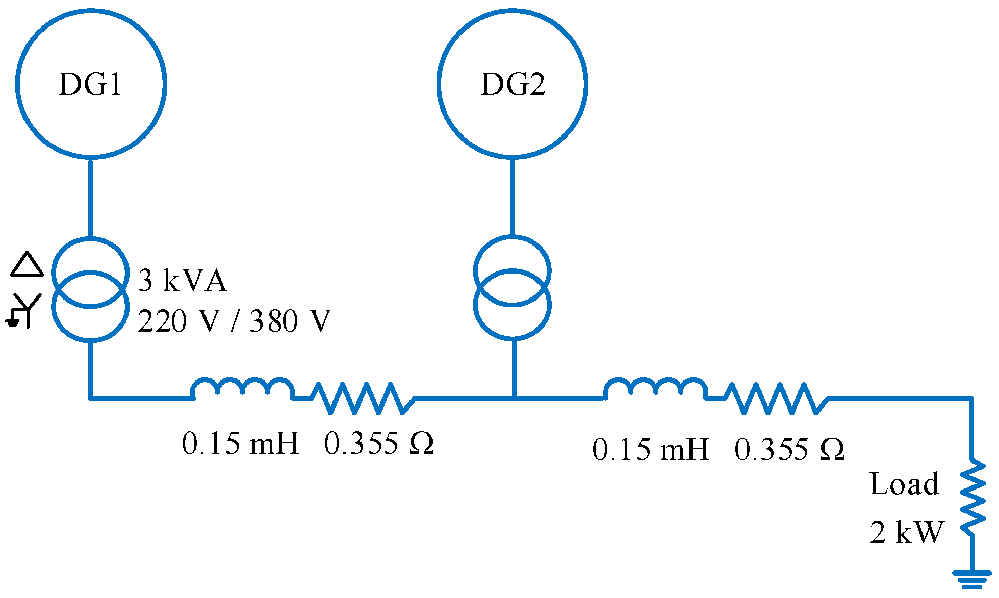
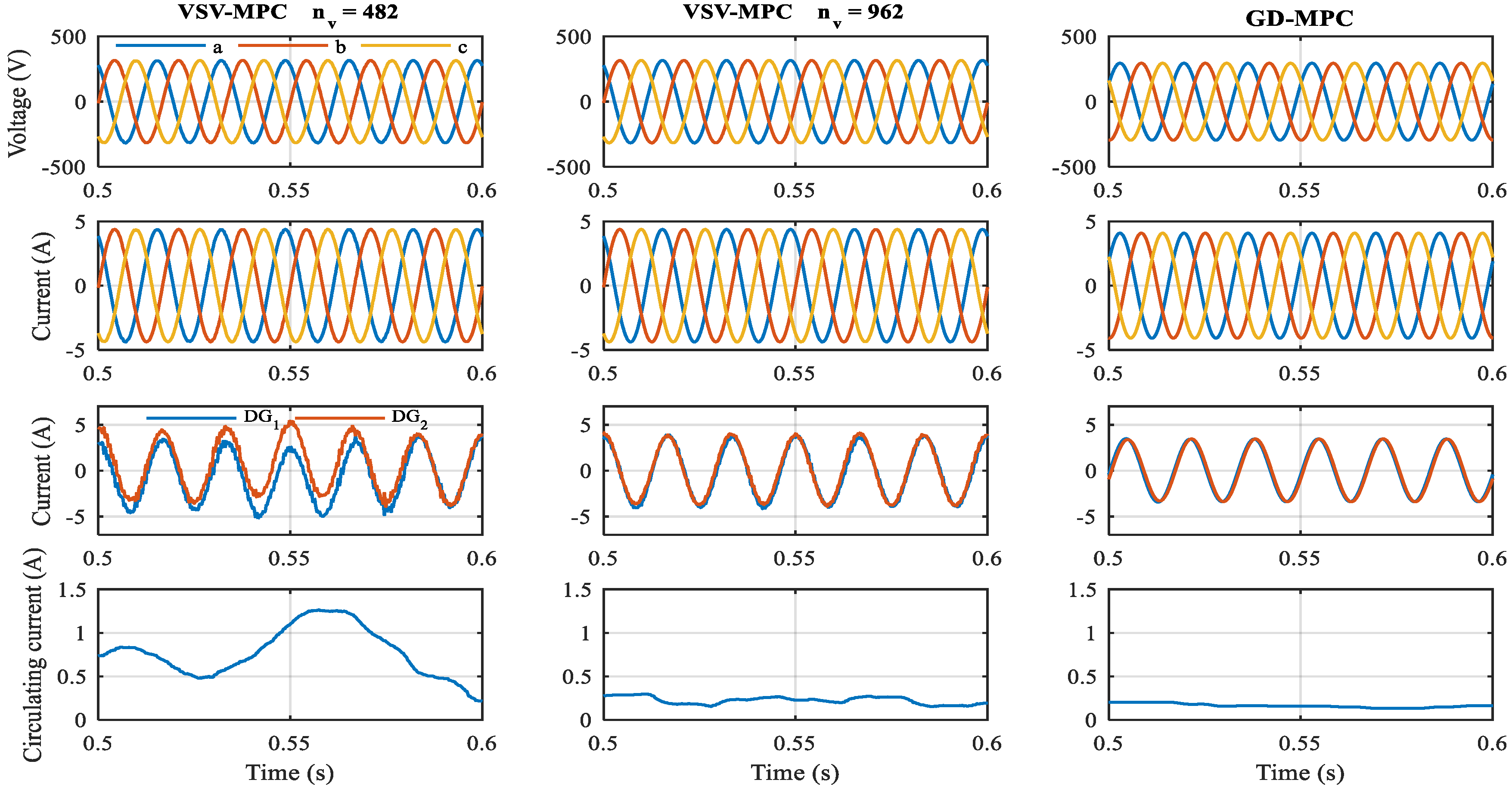
4.2.2. Parallel Operation of Inverters in Microgrid

The parallel operation of the inverter in the MG system is an important issue due to the existence of the circulating current among inverters. The converter controller should be designed properly in order to ensure the stable operation of the MG system and suppress the circulating current. The tested MG system with two parallel inverters shown in Figure 11 is used to evaluate the control performance of the proposed GD-MPC method. A droop control scheme is used to share power between the two inverters. A comparison study of the proposed GD-MPC and VSV-MPC methods is also presented in this section.
The circulating current exists between two parallel inverters due to the line impedance mismatch. Figure 12 shows the results of the two control methods in the tested MG system. As shown in this figure, both GD-MPC and VSV-MPC could stably control the converter in the tested MG system. The output voltage and current of the inverter are sinusoidal. However, the circulating current between two inverters exists, as can be seen in Figure 12. The circulating current in the case of the VSV-MPC method with 482 virtual state vectors is the largest, whereas that in the case of the proposed GD-MPC method is the smallest. The THD value of the output current in the case of the proposed GD-MPC method is smaller than that the case of the VSV-MPC method, with 962 virtual state vectors (1.3% in GD-MPC compared to 1.6% in VSV-MPC, which has 962 vectors).

5. Conclusions

This paper has proposed a new model predictive control strategy for the inverter-based distributed generations in the MG system, which is based on gradient descent (GD) to find the optimal voltage vector. Since the cost function of the MPC method could be formed in the strongly convex function, the optimal voltage vector could be rapidly found by using the GD method. In addition, due to the gradual change of the voltage vector in the normal condition, the convergence speed of the GD method could be improved significantly, and the optimal voltage vector for the next step could be found quickly. A comparison study of the proposed GD-MPC and the VSV-MPC methods has been presented to show the effectiveness of the proposed method. The real-time simulation results have shown that the proposed GD-MPC could significantly reduce the computation time and improve the THD of the output inverter current. Since this paper focused on the design and analysis of the GD-MPC method, the real-time simulation results could be enough to show the advantages of the proposed method. The optimal design and experimental validation of the GD-MPC method on the converter prototype will be considered in our future work.

Author Contributions

The paper was a collaborative effort between the authors. The authors contributed collectively to the theoretical analysis, modeling, simulation, and manuscript preparation.

Funding

This work was supported by the Korea Institute of Energy Technology Evaluation and Planning (KETEP) and the Ministry of Trade, Industry & Energy (MOTIE) of the Republic of Korea (No. 20168530050030).

Conflicts of Interest

The authors declare no conflict of interest.

References

  1. Cort’es, P.; Kazmierkowski, M.P.; Kennel, R.M.; Quevedo, D.E.; Rodr’iguez, J. Predictive control in power electronics and drives. IEEE Trans. Ind. Electron. 2008, 55, 4312–4324. [Google Scholar] [CrossRef]
  2. Kouro, S.; Cort’es, P.; Vargas, R.; Ammann, U.; Rodr’iguez, J. Model predictive control—A simple and powerful method to control power converters. IEEE Trans. Ind. Electron. 2009, 56, 1826–1838. [Google Scholar] [CrossRef]
  3. Nguyen, T.-T.; Yoo, H.-J.; Kim, H.-M. Analyzing the impacts of system parameters on MPC-based frequency control for a stand-alone microgrid. Energies 2017, 10, 417. [Google Scholar] [CrossRef]
  4. Bordons, C.; Montero, C. Basic principles of MPC for power converters: Bridging the gap between theory and practice. IEEE Ind. Electron. 2015, 9, 31–43. [Google Scholar] [CrossRef]
  5. Rodriguez, J.; Kazmierkowski, M.P.; Espinoza, J.R.; Zanchetta, P.; Abu-Rub, H.; Young, H.A.; Rojas, C.A. State of the art of finite control set model predictive control in power electronics. IEEE Trans. Ind. Inform. 2013, 9, 1003–1016. [Google Scholar] [CrossRef]
  6. Li, P.; Li, R.; Feng, H. Total harmonic distortion oriented finite control set model predictive control for single-phase inverters. Energies 2018, 11, 3467. [Google Scholar] [CrossRef]
  7. Sebaaly, F.; Vahedi, H.; Kanaan, H.Y.; Moubayed, N.; Al-Haddad, K. Finite control set model predictive controller for grid connected inverter design. In Proceedings of the 2016 IEEE International Conference on Industrial Technology, Taipei, Taiwan, 14–17 March 2016; pp. 1208–1213. [Google Scholar]
  8. Nguyen, T.-T.; Yoo, H.-J.; Kim, H.-M. Application of model predictive control to BESS for micorgrid control. Energies 20115, 8, 8798–8813. [Google Scholar] [CrossRef]
  9. Hu, S.; Liu, G.; Jin, N.; Gu, L. Constant-frequency model predictive direct power control for fault-tolerant bidirectional voltage-source converter with balanced capacitor voltage. Energies 2018, 11, 2692. [Google Scholar] [CrossRef]
  10. Tomlinson, M.; Mouton, T.; Kennel, R.; Stolze, P. A generic approach to implementing finite-set model predictive control with a fixed switching frequency. In Proceedings of the 2014 IEEE 23rd International Symposium on Industrial Electronic, Istanbul, Turkey, 1–4 June 2014; pp. 330–335. [Google Scholar]
  11. Vazquez, S.; Leon, J.I.; Franquelo, L.G.; Carrasco, J.M.; Martinez, O.; Rodriguez, J.; Cortes, P.; Kour, S. Model predictive control with constant switching frequency using a discrete space vector modulation with virtual state vectors. In Proceedings of the 2009 IEEE International Conference on Industrial Technology, Gippsland, Australia, 10–13 February 2009; pp. 1–6. [Google Scholar]
  12. Nguyen, T.H.; Kim, K.-H. Finite Control Set–Model Predictive Control with Modulation to Mitigate Harmonic Component in Output Current for a Grid-Connected Inverter under Distorted Grid Conditions. Energies 2017, 10, 907. [Google Scholar] [CrossRef]
  13. Tarisciotti, L.; Zanchetta, P.; Watson, A.; Bifaretti, S.; Clare, J.C. Modulated model predictive control for a seven-level cascaded H-bridge back-to-back converter. IEEE Trans. Ind. Electron. 2014, 61, 5375–5383. [Google Scholar] [CrossRef]
  14. Vijayagopal, M.; Empringham, L.; Lillo, L.D.; Tarisciotti, L.; Zanchetta, T.; Wheeler, P. Control of a direct matrix converter induction motor drive with modulated model predictive control. In Proceedings of the 2015 IEEE Energy Conversion Congress and Exposition, Montreal, QC, Canada, 20–24 September 2015; pp. 4315–4321. [Google Scholar]
  15. Tarisciotti, L.; Zanchetta, P.; Watson, A.; Clare, J.C.; Degano, M.; Bifaretti, S. Modulated model predictive control for a three-phase active rectifier. IEEE Trans. Ind. Appl. 2015, 51, 1610–1620. [Google Scholar] [CrossRef]
  16. Rabbeni, R.; Tarisciotti, L.; Gaeta, A.; Formentini, A.; Zanchetta, P.; Pucci, M.; Degano, M.; Rivera, M. Finite states modulated model predictive control for active power filtering systems. In Proceedings of the 2015 IEEE Energy Conversion Congress and Exposition, Montreal, QC, Canada, 20–24 September 2015; pp. 1556–1562. [Google Scholar]
  17. Rivera, M.; Urive, C.; Tarisciotti, L.; Wheeler, P.; Zanchetta, P. Predictive control of an indirect matrix converter operating at fixed switching frequency and unbalanced AC-supply. In Proceedings of the 2015 IEEE International Symposium on Predictive Control of Electrical Drives and Power Electronics, Valparaiso, Chile, 5–6 October 2015; pp. 38–43. [Google Scholar]
  18. Yang, Y.; Wen, H.; Li, D. A fast and fixed switching frequency model predictive control with delay compensation for three-phase inverters. IEEE Access. 2017, 5, 17904–17913. [Google Scholar] [CrossRef]
  19. Cortes, P.; Rodriquez, J.; Quevedo, D.E.; Silva, C. Predictive current control strategy with imposed load current spectrum. IEEE Trans. Power Electron. 2008, 23, 612–618. [Google Scholar] [CrossRef]
  20. Ramirez, R.O.; Espinoza, J.R.; Villarroel, F.A.; Maurelia, E.A.; Reyes, M.E.; Espinosa, E.E. A novel hybrid finite control set model predictive control scheme with reduced switching. IEEE Trans. Ind. Electron. 2013, 61, 5912–5920. [Google Scholar] [CrossRef]
  21. Rubinic, J.; Yaramasu, V.; Wu, B.; Zargari, N. Model predictive control of neutral-point clamped inverter with harmonic spectrum shaping. In Proceedings of the 2015 IEEE Energy Conversion Congress and Exposition, Montreal, QC, Canada, 20–24 September 2015. [Google Scholar]
  22. Song, Z.; Xia, C.; Liu, T. Predictive current control of three-phase grid-connected converters with constant switching frequency for wind energy systems. IEEE Trans. Ind. Electron. 2013, 60, 2451–2464. [Google Scholar] [CrossRef]
  23. Aguirre, M.; Kouro, S.; Rojas, C.A.; Rodriquez, J.; Leon, J.I. Switching frequency regulation for FCS-MPC based on a period control approach. IEEE Trans. Ind. Electron. 2018, 65, 5764–5773. [Google Scholar] [CrossRef]
  24. Xue, C.; Song, W.; Wu, X.; Feng, X. A Constant switching frequency finite-control-set predictive current control scheme of a five-phase inverter with duty ratio optimization. IEEE Trans. Power Electron. 2018, 33, 3583–3594. [Google Scholar] [CrossRef]
  25. Xia, C.; Liu, T.; Shi, T. A simplified finite-control-set model-predictive control for power inverters. IEEE Trans. Ind. Inform. 2014, 10, 991–1002. [Google Scholar]
  26. Zhang, Y.; Xie, W.; Li, Z. Low-complexity model predictive power control: Double-vector-based approach. IEEE Trans. Ind. Electron. 2014, 61, 5871–5880. [Google Scholar] [CrossRef]
  27. Balamurali, A.; Feng, G.; Lai, C.; Tjong, J.; Akr, N.C. Maximum efficiency control of PMSM drives considering system losses using gradient descent algorithm based on dc power measurement. IEEE Trans. Energy Convers. 2018, 33, 2240–2249. [Google Scholar] [CrossRef]
Figure 1. Space vector diagram in αβ frame including virtual states.
Energies 12 01156 g001
Figure 2. Space vector diagram in the αβ frame, including virtual states.
Energies 12 01156 g002
Figure 3. Example of a gradient search for a stationary point.
Energies 12 01156 g003
Figure 4. Space vector diagram in the αβ frame, including virtual vector states.
Energies 12 01156 g004
Figure 5. Flowchart of the proposed control strategy.
Energies 12 01156 g005
Figure 6. Effect of learning rate γ on the control performance of the converter.
Energies 12 01156 g006
Figure 7. The effect of uncertain parameters on the control performance.
Energies 12 01156 g007
Figure 8. Performance of the proposed model predictive control (MPC) in the condition of nonlinear load.
Energies 12 01156 g008
Figure 9. Computation time of the proposed gradient descent model predictive control (GD-MPC), virtual state vector model predictive control (VSV-MPC), and conventional model predictive control (MPC).
Energies 12 01156 g009
Figure 10. Comparison on the proposed GD-MPC method and the VSV-MPC method.
Energies 12 01156 g010
Figure 11. Tested microgrid (MG) system with two parallel inverters.
Energies 12 01156 g011
Figure 12. Control performance of the proposed GD-MPC and VSV-MPC in the MG system with two parallel inverters.
Energies 12 01156 g012
Table 1. System parameters.
SymbolParameterValue
-Rating Power3 kW
V *Nominal Bus Voltage380 V
f *Nominal Bus Frequency60 Hz
VdclinkDC Link Voltage380 V
Lf, CfLC Filter of DGs2 mH, 40 uF
fsSwitching Frequency10 kHz
-Transformer220(Δ)/380(Y)
Rl, LlLine Impedance0.355 Ω, 0.15 mH
TsSampling Time100 μs

