Dynamic Optimization of Boil-Off Gas Generation for Different Time Limits in Liquid Natural Gas Bunkering


Abstract
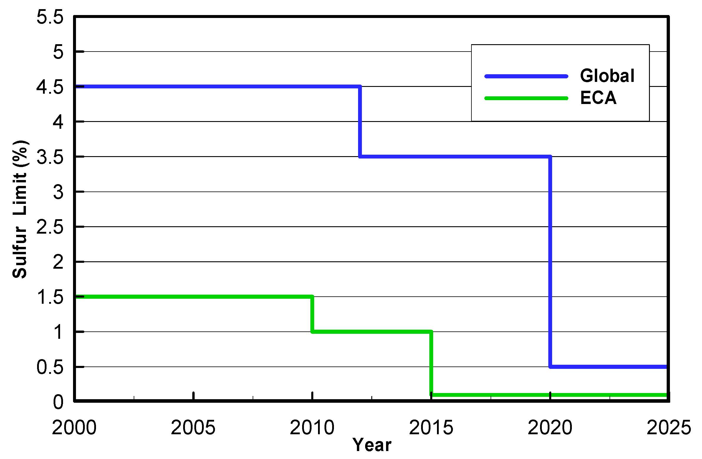
:1. Introduction
2. System Model and Procedure Design
2.1. Tank Geometry
2.2. Determination of LNG Flow Rate
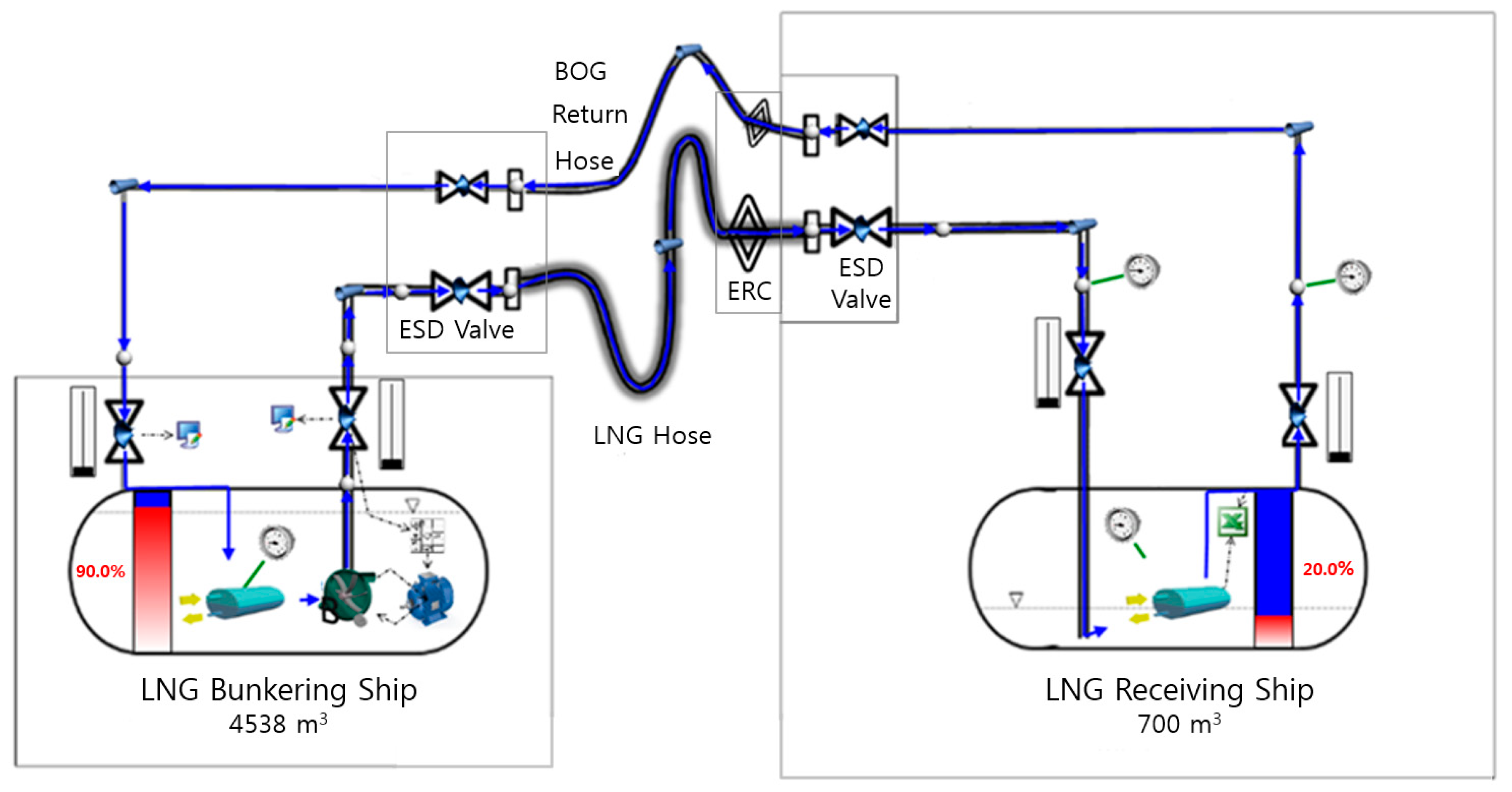
2.3. Pipeline System Design
- Mass Flow Rate:
- Transfer rate:
- Pipeline diameter:where presents the mass flow rate; is the volume flow rate; is the mass density of LNG bunker; is the velocity of LNG; is the diameter of pipeline.
3. Dynamic Simulation
3.1. Dynamic Simulation Method
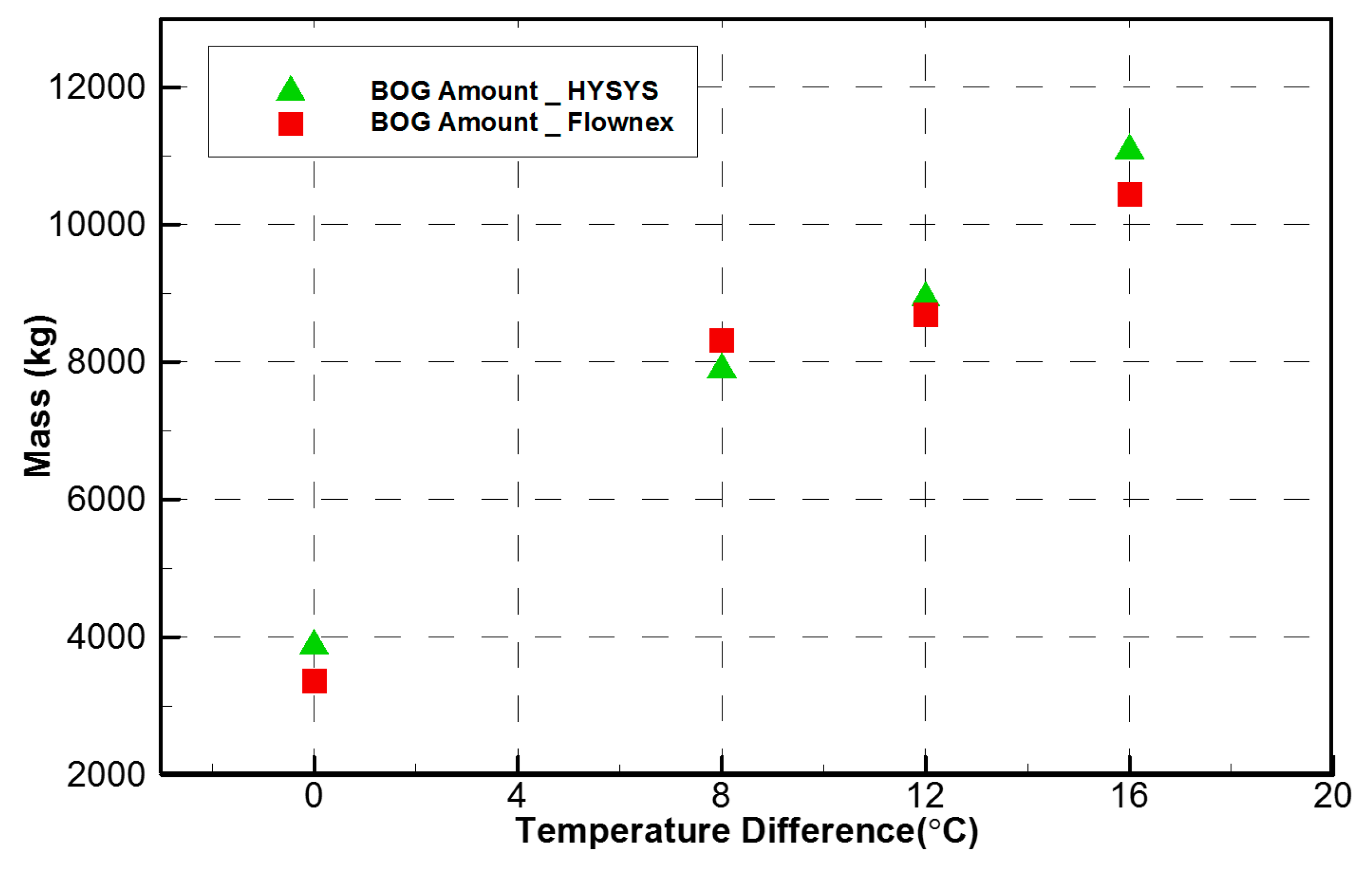
3.2. Code Validation
4. Results and Discussion
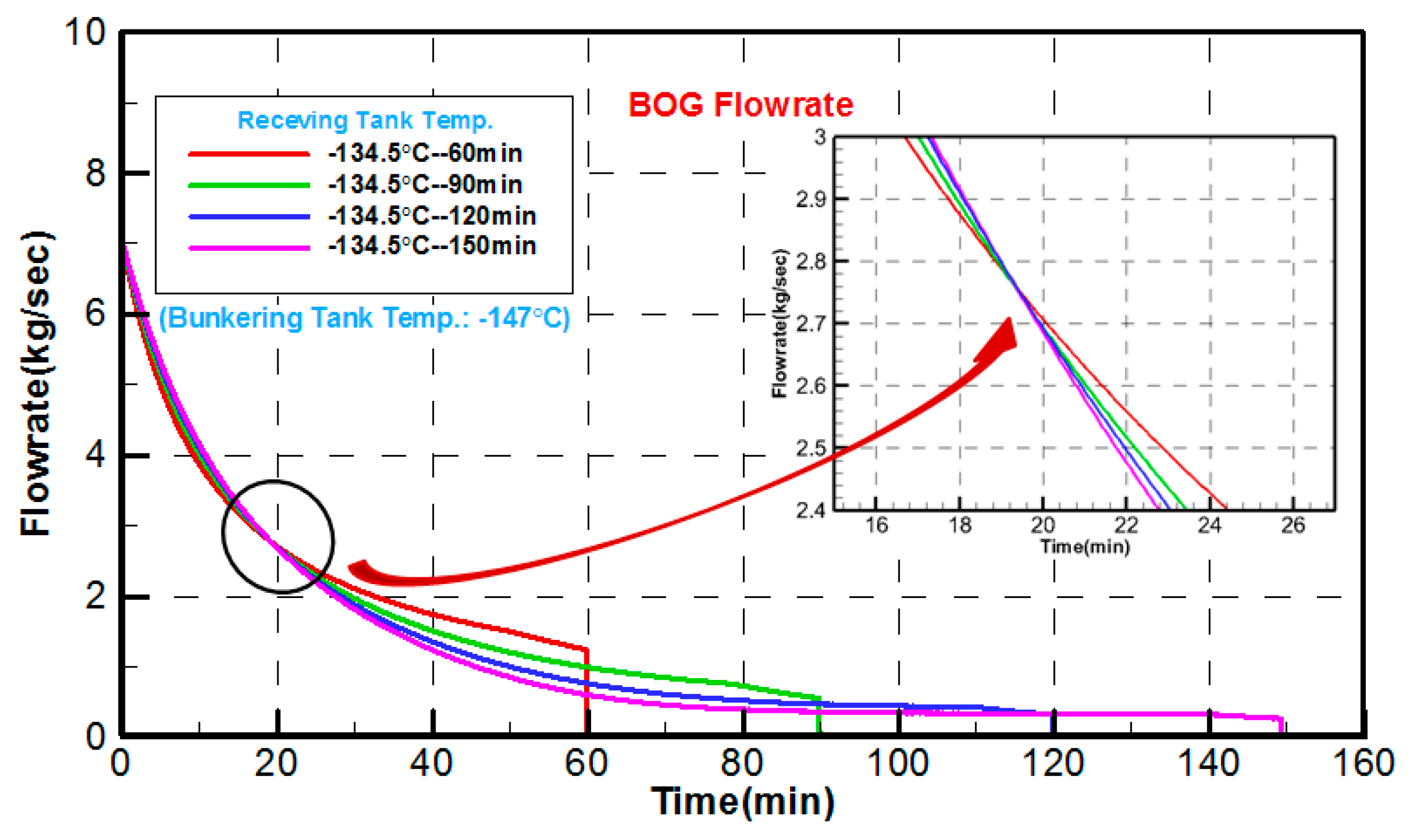
4.1. Transient BOG Variation
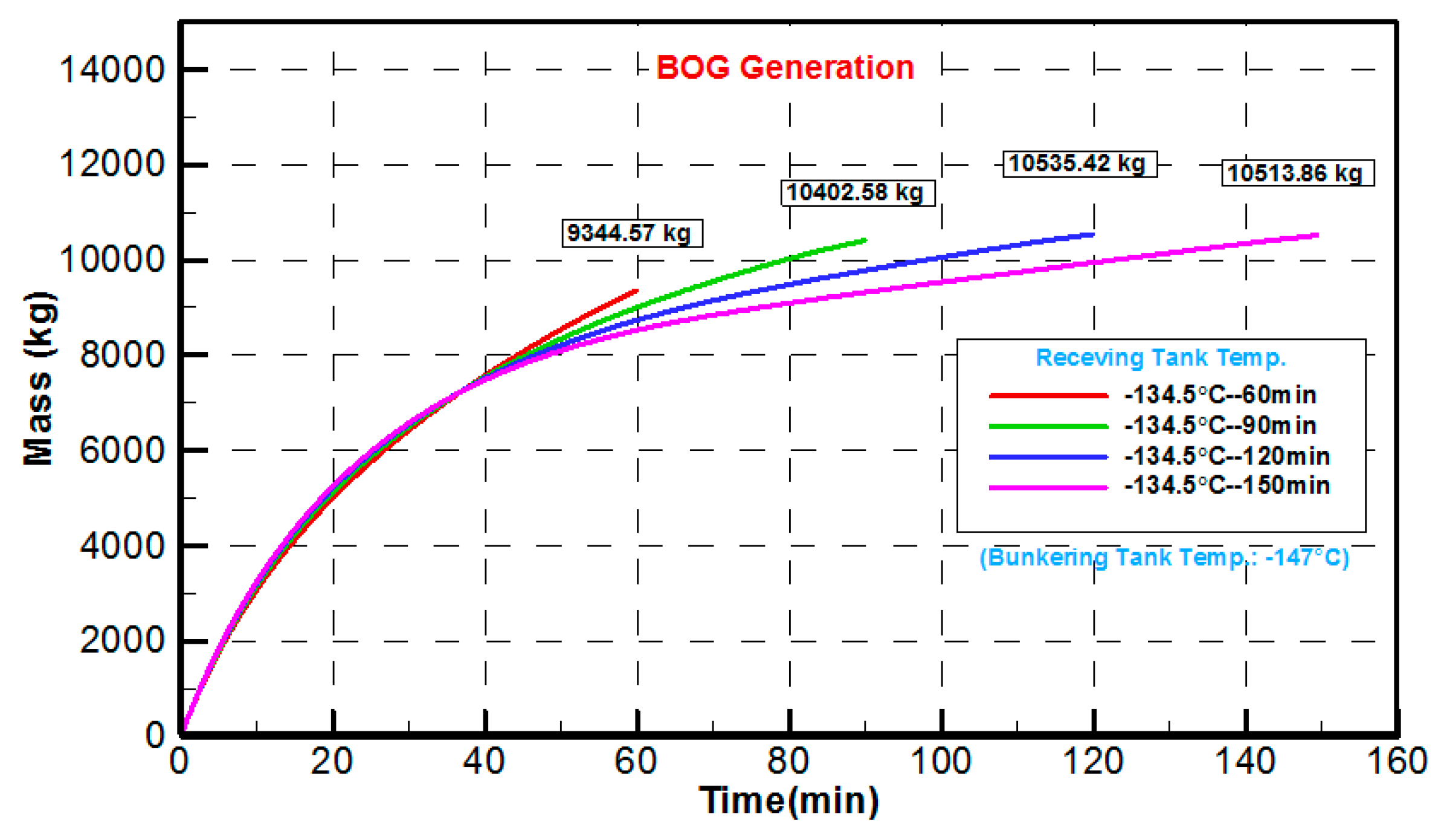
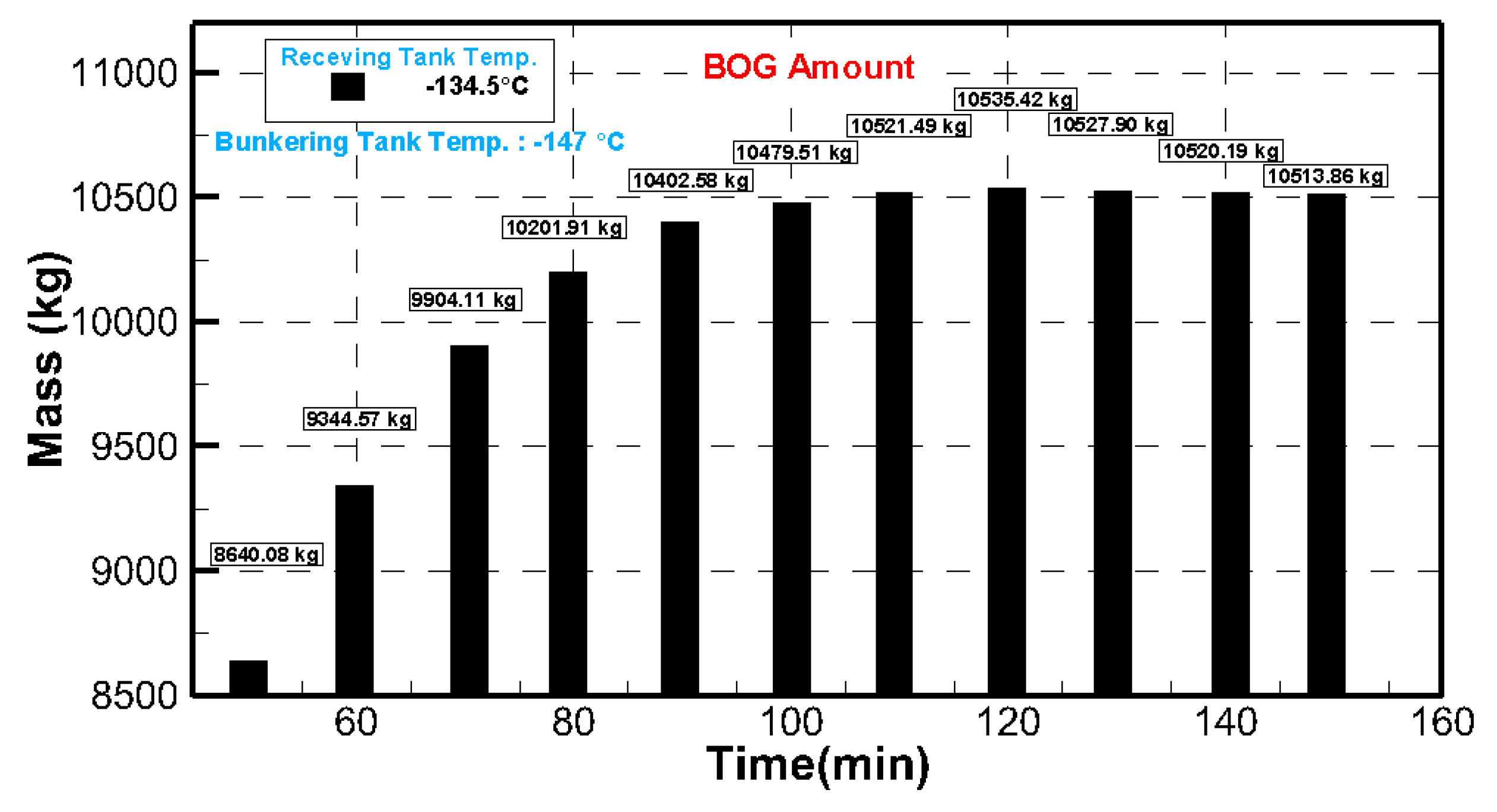
4.2. BOG Generation
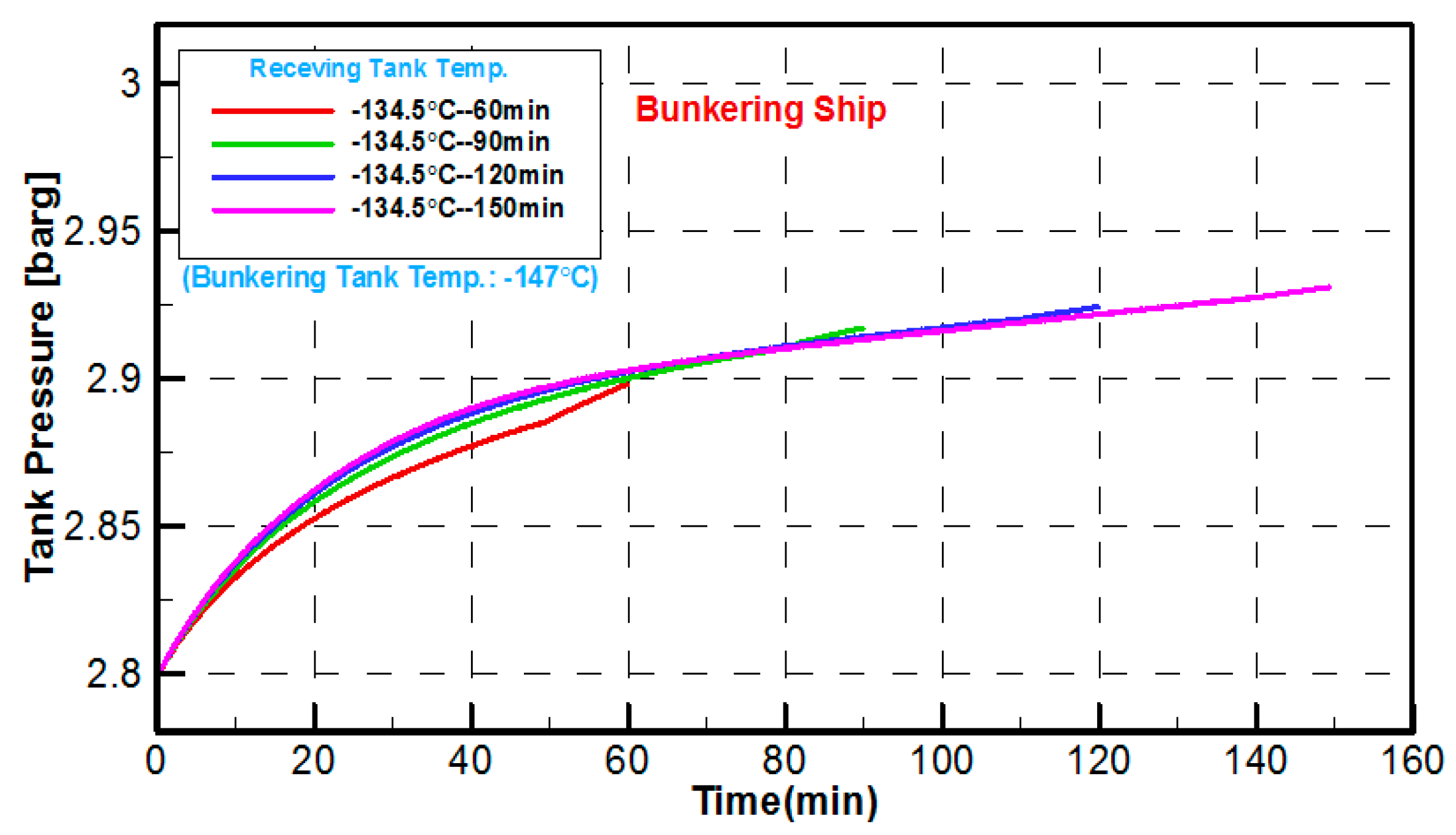
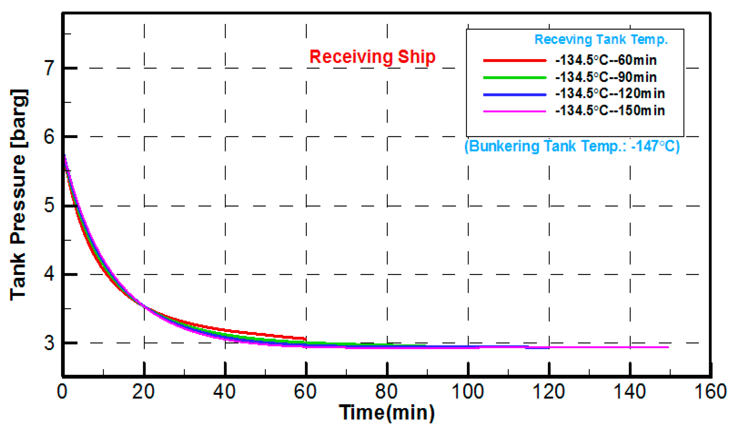
4.3. Variations in the Bunker and Receiver Tank Pressure
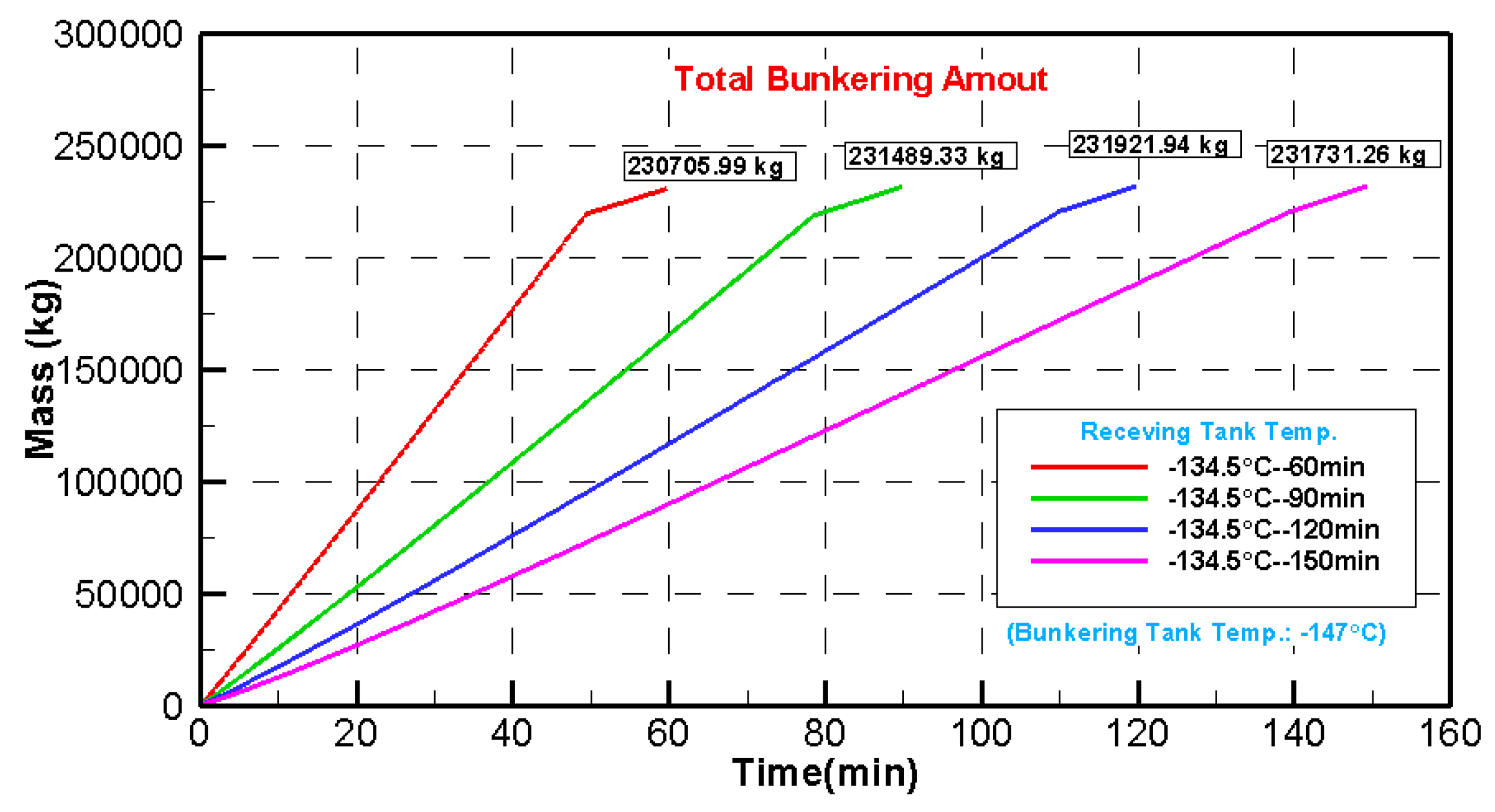
4.4. LNG Flow Rate and Total LNG Bunkering Amount
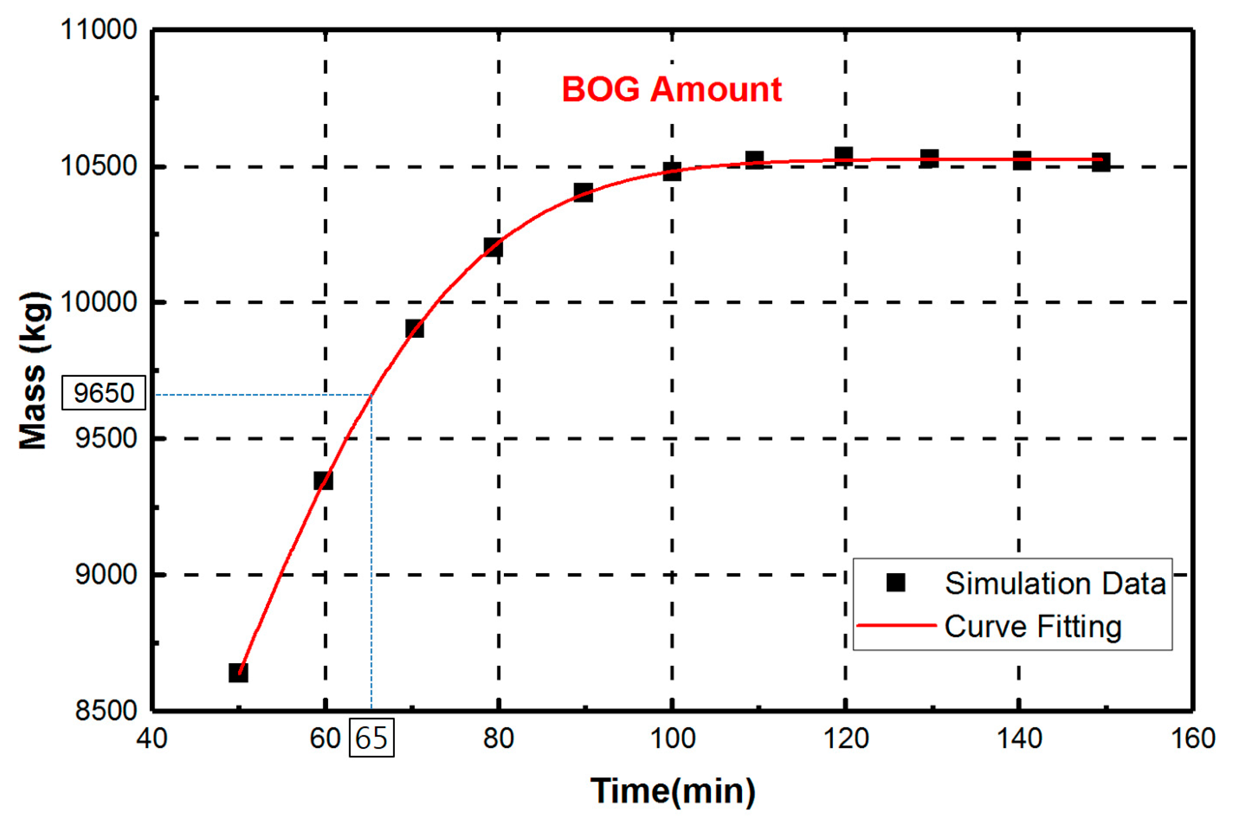
4.5. Calculation for Mass of BOG Amount
5. Conclusions
Author Contributions
Acknowledgments
Conflicts of Interest
Nomenclature
| BOG | Boil-off Gas |
| BL | Bunkering Limit |
| CFD | Computational Fluid Dynamics |
| CH4 | Methane |
| ECAs | Emission Control Areas |
| ESD | Emergency Shutdown |
| ERC | Emergency Release Coupling |
| FL | Filling Limit |
| JBOG | Jetty Boil-off Gas |
| HFO | Heavy Fuel Oil |
| IMO | International Maritime Organization |
| IQRA | Integrated Quantitative Risk Assessment |
| LNG | Liquefied Natural Gas |
| LNG-FPSO | Floating Production Storage and Offloading unit for Liquefied Natural Gas |
| MGO | Marine Gas Oil |
| PBMR | Pebble Bed Modular Reactor Company |
| PFD | Process Flow Diagram |
| PTS | Pipeline-to-Ship |
| SOx | Sulphur Oxide |
| SRK | Soave-Redlich-Kwong equation |
| STS | Ship-to-Ship |
| SWeibull 2 | Sigmoidal Weibull function type 2 |
| TTS | Truck-to-Ship |
Symbols
∆p ∆t | Energy parameter Alpha function Size parameter Diameter of pipeline Pressure difference Temperature difference Function of Mass flow rate Mass of BOG Pressure Pressure at critical point LNG density at bunkering temperature LNG density at reference temperature Volume flow rate Gas Constant Temperature Temperature at critical point Time Velocity Molar volume Acentric factor |
References
- Wang, S.Y.; Notteboom, T. The Adoption of Liquefied Natural Gas as a Ship Fuel: A Systematic Review of Perspectives and Challenges. Transp. Rev. 2014, 34, 749–774. [Google Scholar] [CrossRef]
- Adachi, M.; Kosaka, H.; Fukuda, T.; Ohashi, S.; Harumi, K. Economic analysis of trans-ocean LNG-fueled container ship. J. Mar. Sci. Technol. 2014, 19, 470–478. [Google Scholar] [CrossRef]
- Notteboom, T. The impact of low sulphur fuel requirements in shipping on the competitiveness of roro shipping in Northern Europe. WMU J. Marit. Aff. 2011, 10, 63–95. [Google Scholar] [CrossRef]
- Xu, J.Y.; Fan, H.J.; Wu, S.P.; Shi, G.Z. Research on LNG Ship to Ship (STS) Bunkering Operations. J. Ship Eng. 2015, 1, 7–10. [Google Scholar]
- Lee, M.H.; Shao, Y.D.; Kim, Y.T.; Kang, H.K. Performance characteristics under various load conditions of coastal ship with LNG-powered system. J. Korean Soc. Mar. Eng. 2017, 5, 424–430. [Google Scholar] [CrossRef]
- IMO. Sulphur Oxides (SOx) and Particulate Matter (PM)—Regulation 14. Available online: http://www.imo.org/en/OurWork/Environment/PollutionPrevention/AirPollution/Pages/Sulphur-oxides-(SOx)-%E2%80%93-Regulation-14.aspx (accessed on 20 April 2018).
- ABS. LNG bunkering: Technical and Operational Advisory; ABS: Houston, TX, USA, 2014. [Google Scholar]
- Ryu, J.H. Concept for Protection against Overpressure Caused by BOG Generated during Ship-to-Ship LNG Bunkering. Master’s Thesis, Korea Advanced Institute of Science and Technology (KAIST), Daejeon, Korea, 2012. [Google Scholar]
- Shao, Y.D.; Kang, H.K.; Yoon, S.D.; Kim, Y.T. Dynamic Simulation for Boil-off Gas in LNG Fueled Ship during Ship-to-ship Bunkering Process. In Proceedings of the International Symposium on Marine Engineering (ISME), Tokyo, Japan, 15–19 October 2017; Japan Institute of Marine Engineering (JIME): Tokyo, Japan, 2017. [Google Scholar]
- Yun, S.; Ryu, J.; Seo, S.; Lee, S.; Chung, H.; Seo, Y.; Chang, D. Conceptual design of an offshore LNG bunkering terminal: A case study of Busan Port. J. Mar. Sci. Technol. 2015, 2, 226–237. [Google Scholar] [CrossRef]
- Zakaria, M.; Osman, K.; Yusof, A.; Hanafi, H.; Saadun, M.; Manaf, M. Parametric analysis on boil-off gas rate inside liquefied natural gas storage tank. J. Mech. Eng. Sci. 2014, 6, 845–853. [Google Scholar] [CrossRef]
- Bahgat, W.M. Proposed method for dealing with boil-off gas on board LNG carriers during loaded passage. Int. J. Multidiscip. Curr. Res. 2015, 3, 508–512. [Google Scholar] [CrossRef]
- Fan, H.; Cheng, K.; Wu, S. CFD based simulation of LNG release during bunkering and cargo loading/unloading simultaneous operations of a containership. J. Ship. Ocean Eng. 2017, 7, 51–58. [Google Scholar]
- Sun, B.; Guo, K.; Pareek, V.K. Hazardous consequence dynamic simulation of LNG spill on water for ship-to-ship bunkering. Process Saf. Environ. Prot. 2017, 107, 402–413. [Google Scholar] [CrossRef]
- Jeong, B.; Lee, B.S.; Zhou, P.; Ha, S. Evaluation of safety exclusion zone for LNG bunkering station on LNG-fuelled ships. J. Mar. Eng. Technol. 2017, 4177, 1–24. [Google Scholar] [CrossRef]
- Kurle, Y.M.; Wang, S.; Xu, Q. Simulation study on boil-off gas minimization and recovery strategies at LNG exporting terminals. Appl. Energy 2015, 156, 628–641. [Google Scholar] [CrossRef]
- Kurle, Y.M.; Wang, S.; Xu, Q. Dynamic simulation of LNG loading, BOG generation, and BOG recovery at LNG exporting terminals. Comput. Chem. Eng. 2017, 97, 47–58. [Google Scholar] [CrossRef]
- Hasan, M.M.F.; Zheng, A.M.; Karimi, I.A. Minimizing boil-off losses in liquefied natural gas transportation. Ind. Eng. Chem. Res. 2009, 48, 9571–9580. [Google Scholar] [CrossRef]
- Yan, G.; Gu, Y. Effect of parameters on performance of LNG-FPSO offloading system in offshore associated gas fields. Appl. Energy 2010, 87, 3393–3400. [Google Scholar] [CrossRef]
- International Maritime Organization. International Code for the Construction and Equipment of Ships Carrying Liquefied Gas in Bulk; IMO: London, UK, 2003. [Google Scholar]
- Aspen Technology. Aspen. HYSYS Operations Guide; V10; Aspen Technology Inc.: Burlington, MA, USA, 2017. [Google Scholar]
- ISO 20519:2017. Ships and Marine Technology—Specification for Bunkering of Liquefied Natural Gas Fueled Vessels, 1st ed.; ISO: Geneva, Switzerland, 2017. [Google Scholar]
- Li, Y.J.; Chen, X.S. Dynamic Simulation for Improving the Performance of Boil-Off Gas Recondensation System at LNG Receiving Terminals. Chem. Eng. Comm. 2012, 10, 1251–1262. [Google Scholar] [CrossRef]
- Soave, G. Equilibrium constants from a modified Redlich-Kwong equation of state. Chem. Eng. Sci. 1972, 6, 1197–1203. [Google Scholar] [CrossRef]
- Stryjek, R.; Vera, J.H. PRSV: An Improved Peng- Robinson Equation of State for Pure Compounds and Mixtures. Can. J. Chem. Eng. 1986, 64, 323–333. [Google Scholar] [CrossRef]
- Lee, S.; Jeon, J.; Lee, U.; Lee, C. A Novel Dynamic Modeling Methodology for Boil-Off Gas Recondensers in Liquefied Natural Gas Terminals. J. Chem. Eng. Jpn 2015, 48, 841–847. [Google Scholar] [CrossRef]
- Effendy, S.; Khan, M.S.; Farooq, S.; Karimi, I.A. Dynamic modelling and optimization of an LNG storage tank in a regasification terminal with semi-analytical solutions for N 2-free LNG. Comput. Chem. Eng. 2017, 99, 40–50. [Google Scholar] [CrossRef]
- Shariq, M.; Effendy, S.; Karimi, I.A.; Wazwaz, A. Improving design and operation at LNG regasification terminals through a corrected storage tank model. Appl. Therm. Eng. 2019, 149, 344–353. [Google Scholar]
- Park, C.; Cho, B.; Lee, S.; Kwon, Y. Study on the Re-liquefaction Processing for Boil off Gas System of Floating Offshore LNG Bunkering Terminal. In Proceedings of the Twenty-sixth International Ocean and Polar Engineering Conference, Roodes, Greece, 26 June–1 July 2016; International Society of Offshore and Polar Engineers (ISOPE): Mountain View, CA, USA, 2016. [Google Scholar]
- Ravenswaay, J.P.; Greyvenstein, G.P.; Neikerk, W.M.K.; Labuschagne, J.T. Verification and validation of the HTGR systems CFD code Flownex. Nucl. Eng. Des. 2006, 5–6, 491–501. [Google Scholar] [CrossRef]
- Dobrata, L.B.; Komar, I. Problem of Boil-off in LNG Supply Chain. J. Trans. Marit. Sci. 2013, 2, 91–100. [Google Scholar] [CrossRef]
- Shao, Y.D.; Lee, Y.H.; Kim, Y.T.; Kang, H.K. Parametric Investigation of BOG Generation for Ship-to-Ship LNG Bunkering. J. Korean Soc. Mar. Environ. Saf. 2018, 3, 352–359. [Google Scholar] [CrossRef]
- Seo, Y.; Lee, S.; Kim, J.; Huh, C.; Chang, D. Determination of optimal volume of temporary storage tanks in a ship-based carbon capture and storage (CCS) chain using life cycle cost (LCC) including unavailability cost. Int. J. Greenh. Gas Control 2017, 64, 11–22. [Google Scholar] [CrossRef]
- Nguyen, L.; Kim, M.; Choi, B. An experimental investigation of the evaporation of cryogenic-liquid- pool spreading on concrete ground. Appl. Therm. Eng. 2017, 123, 196–204. [Google Scholar] [CrossRef]


| Parameter | Value | Tank Type | |
|---|---|---|---|
| Bunkering Ship | Tank volume [m3] | 4538 | IMO Type C |
| Diameter [m] | 12.0 | ||
| Length [m] | 40.12 | ||
| Receiving Ship | Tank volume [m3] | 700 | |
| Diameter [m] | 8.0 | ||
| Length [m] | 13.93 | ||
| Bunkering Time Limit [min.] | Initial Mass Flow Rate [kg/h] | Mass Flow Rate [kg/h] (After Tank’s Level of Receiving Ship Over 85%) |
|---|---|---|
| 60 | 280,000 | 72,000 |
| 90 | 180,000 | |
| 120 | 125,000 | |
| 150 | 100,000 |
| Modeling of System Startup | Conditions for the Initial Bunkering Dtartup | (1) Conditions (pressure/quality) in the receiver tank and bunker tank should be in a stable state. |
| (2) BOG return line/LNG bunker line should be closed. | ||
| Procedure Change | (1) Open BOG valve (bunker tank side and receiver tank side) for 10 s. | |
| (2) Start the heat ingress in the bunker and receiver tank. | ||
| (3) Open the LNG Bunkering valve (receiver tank side) for 10 s. | ||
| (4) Start the LNG bunkering pump (8.9 s after startup) and operate the flow controller 9 s after the starting point. | ||
| (5) Open the LNG bunkering valve (bunker tank side) for 10 s. | ||
| Modeling of System Shutdown | Procedure Change | (1) When the level of LNG fuel tank for the receiving ship reaches 85%, the mass flow rate ramps down to 72,000 kg/h. |
| (2) When the level of the LNG fuel tank for the receiving ship reaches 89.99%, controller cut-off occurs. | ||
| (3) When the level of LNG fuel tank for receiving ship tank reaches 90%, the pump power cut-off occurs and all valves are closed for 20 s to prevent the surge phenomena. | ||
| Simulation Control | (1) The size of the time step (Adaptive time stepping) is adjusted to 100–1,000 ms. | |
| (2) Setting of the Simulation Stop: Finish filling and close all valves and then stop the system after 30 s. |
| Bunkering Ship (4538 m3) | Receiving Ship (700 m3) | ||
|---|---|---|---|
| Begin Bunkering | Tank level (%) | 90.0 | 20.0 |
| Temperature (°C) | −147.0 | −134.5 | |
| Tank pressure (barg) | 2.8 | 5.8 | |
| Finish Bunkering | Tank level (%) | 77.1 | 90.0 |
| Temperature (°C) | −146.4 | −145.6 | |
| Tank pressure (barg) | 2.9 | 3.1 | |
| Bunkering Time Limit (min.) | 60 | 90 | 120 | 150 | |
|---|---|---|---|---|---|
| BOG Amount (kg) | 9344.57 | 10402.58 | 10535.42 | 10513.86 | |
| Tank Pressure (Barg) | Bunkering Ship | 2.90 | 2.93 | 2.93 | 2.93 |
| Receiving Ship | 3.06 | 2.99 | 2.97 | 2.94 | |
| Total Bunkering Amount (kg) | 230705.99 | 231489.33 | 231921.94 | 231731.26 | |
© 2019 by the authors. Licensee MDPI, Basel, Switzerland. This article is an open access article distributed under the terms and conditions of the Creative Commons Attribution (CC BY) license (http://creativecommons.org/licenses/by/4.0/).
Share and Cite
Shao, Y.; Lee, Y.; Kang, H. Dynamic Optimization of Boil-Off Gas Generation for Different Time Limits in Liquid Natural Gas Bunkering. Energies 2019, 12, 1130. https://doi.org/10.3390/en12061130
Shao Y, Lee Y, Kang H. Dynamic Optimization of Boil-Off Gas Generation for Different Time Limits in Liquid Natural Gas Bunkering. Energies. 2019; 12(6):1130. https://doi.org/10.3390/en12061130
Chicago/Turabian StyleShao, Yude, Yoonhyeok Lee, and Hokeun Kang. 2019. "Dynamic Optimization of Boil-Off Gas Generation for Different Time Limits in Liquid Natural Gas Bunkering" Energies 12, no. 6: 1130. https://doi.org/10.3390/en12061130
APA StyleShao, Y., Lee, Y., & Kang, H. (2019). Dynamic Optimization of Boil-Off Gas Generation for Different Time Limits in Liquid Natural Gas Bunkering. Energies, 12(6), 1130. https://doi.org/10.3390/en12061130