Simultaneous Power Flow Decouple and Converter Gain Design for Electric Vehicle to Grid System

Abstract

This paper presents a novel idea based on the Port-Hamiltonian and cascade system to control the electric vehicle-to-grid (V2G) system. Based on the proposed method, the relationship between the converter plant gain and the moment of inertia of generator that has been established is effective for decoupled control of the V2G system. It is well known that the existing methods apply the $H_{\infty }$ control and PSO method to enumerate and choose the value of converter plant gain from the region decided by the state of charge. Since an explicit form of converter plant gain is obtain in this paper, the proposed method that is unnecessary to repeat the above existing details effectively reduces the calculated amount of converter plant gain. Finally, the simulations demonstrate the validity and advantage of the proposed method.

1. Introduction

Electric vehicles (EVs) that plug into power grids are considered as the mobile energy stored equipments for the power systems. Therefore, a vehicle-to-grid (V2G) system that contains EVs and power systems is studied by the researchers [1,2,3]. Noting a V2G system, its power systems that are constructed by a single area or multi-area power system apply load frequency control (LFC) method to finish frequency regulation and systemic stability [4,5,6,7]. Meanwhile, when EVs charge or discharge, their batteries subjected to the state of charge (SOC) or not participate in frequency regulation of power systems [8,9,10,11]. Due to the above facts, frequency regulation is useful to analyze and control a V2G system. Moreover, a V2G system faces some practical operating conditions, e.g., the new energies [3,12] and time delay [13,14,15]. Thus, the researchers consider the V2G system as a whole one and directly design some control laws to stabilize it [12,13,14,15,16,17].

Though the above results [12,13,14,15,16,17] present some results for a V2G system, there are some flaws in my outlooks. The first one is that the existing methods design control laws by feedback of area control errors (ACE) [12,13,14,15,16,17], and the second one is that the existing results enumerate the gain of converter plant from the region $[0,1]$ restricted by the SOC [12,13,14,15,16,17], at last, the existing results apply $H_{\infty }$ control to design the control law for V2G and multi-area LFC system, respectively [12,13,14,15,16,17]. Noted a V2G system, every single area LFC system connects with EVs. Consequently, EVs influence the frequency incremental of themselves areas firstly, then, affect frequency incremental of other areas via power flow lines. Unluckily, the existing results [12,13,14,15,16,17] that do not decouple the power flow contained by ACE bring j areas’s frequency incremental to i area. This fact can be addressed as a decoupled problem of power flows. Without EVs, a decoupled method for multi-area LFC system has been reported [7], while the decoupled problem V2G system is not work out. For a V2G system, since the converter plant gain can be designed via power electronics and control method [18,19,20], it is better to design a useful expression of converter plant gain and to avoid enumerating its value from the above region. Especially for the last defect, EVs that are considered as mobile energy stored equipments can be considered as the disturbances for the LFC system. In control theory, since there are robust control laws for the LFC system [4,5,6,7], those methods that should also satisfy for V2G system are not necessary to be designed again. However, the existing methods that implement $H_{\infty }$ and LFC control to compute the control laws for a V2G system obviously enlarges the computing amount. Therefore, this paper proposes some new control methods to work out the aforementioned flaws.

To achieve the above goals, a V2G system in this paper is designed without and with SOC. When a V2G system is without SOC, it is considered as two cascaded subsystems, i.e., the governor of V2G system is addressed as the first subsystem and the others of V2G system are the second subsystem. Between the two subsystems, the interconnection channel is the output and input channel between governor and turbine. According to the features of Port-Hamiltonian (PH) system [7,21], an converter gain is designed in a fraction form, which denominator is the moment of inertia of generator and numerator is the time constant of converter. Meanwhile, the input of turbine is designed by the PH system, which assures that the second subsystem is asymptotical stability. Due to the cascaded channel between the two above subsystems, the output of governor that is equal to input of turbine yields a control law to asymptotically stabilize the first subsystem constructed by governor. Based on the feature of cascaded systems [22], once two cascaded subsystems are asymptotically stable, the whole system containing the two above subsystems is asymptotically stable. Namely, the V2G system not subjected to SOC is asymptotically stable. When a V2G system subjects to SOC, the batteries of EVs are restricted by power limitation, which is a saturation function with a region $[0,1]$. Since an explicit expression for plant gain is designed, it is necessary to check whether its value satisfies the above region or not. In theory, the unit of moment of inertia of generator is often chosen as second (s) [4], while the unit of time constant of converter is often chosen as millisecond (ms) [20]. According to the expression of converter plant gain designed by proposed method and the two above units, its value can belong to the region $[0,1]$. In application, the values of time constant of converter and moment of inertia of generator are detectable. Thus, the value of converter plant gain designed by the proposed method not only satisfies the above region, but also is realizable. As we all know, the V2G system not restricted by SOC has a similar state equation as the state equation of V2G system restricted by SOC. The latter system only needs to consider the value of plant gain belonging to the above region. Since the value of converter plant gain satisfies that restriction, the proposed method is also effective for the V2G system restricted by SOC.

Compared with the existing results, the proposed method has three advantages. The first that is decoupling of power flow avoids the feedback of j area’s frequency incremental being used in the i area, the second that is designing an useful expression of converter plant gain avoids to randomly enumerating the value of the above gain from the region decided by SOC, and the last is the proposed method satisfying for both of V2G and LFC system, while the existing methods should design the control laws for V2G and LFC system, respectively. Thus, the proposed method effectively reduces the computing amounts. At last, simulations show the validity and benefit of the proposed method.

2. Background

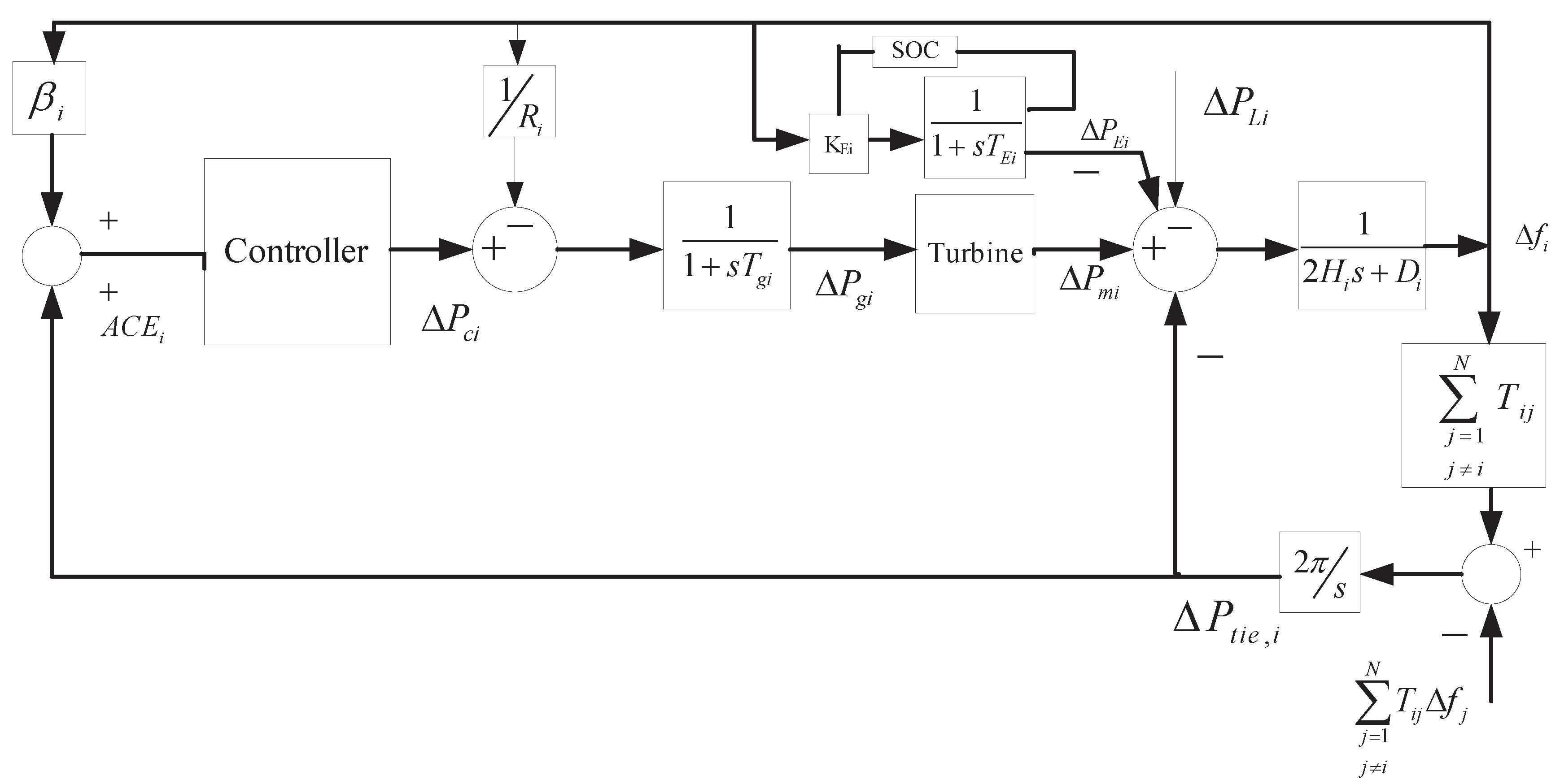
Here, a block control diagram of ith area of V2G system that is shown in the following Figure 1 can be casted into two parts, i.e., LFC and EVs.

For one part, there are transfer functions and controller of LFC [4]. In details, $\Delta f_i$, $\Delta P_{mi}$, $\Delta P_{gi}$ and $\Delta P_{Li}$ are the deviation of frequency, the generator mechanical output, valve position, and load in the area i, respectively. $H_i$, $D_i$, $T_{gi}$, $T_{ti}$, $R_i$ and ${\beta }_i$ denote the moment of inertia of the generator, generator damping coefficient, time constant of the governor, time constant of the turbine, speed drop, and frequency bias factor in the area i, respectively. $\Delta P_{ci}$ is the control input. Once $\Delta f_i$ and $\Delta P_{tie,i}$ are feedbacks to the area control error $AC{E}_i$, there is $AC{E}_i={\beta }_i\Delta f_i+\Delta P_{tie,i}$ with ${\beta }_i=\frac{1}{R_i}+D_i$. For other part, $\Delta P_{Ei}$ that are power of EVs in the area i is as follows $\Delta P_{Ei}={\sum }_{k=1}^N{\lambda }_k\Delta P_{Ei,k}$, where $\Delta P_{Ei,k}$, ${\lambda }_k$ and N mean that the power of kth EV plugged to area i LFC system, status of kth EV and numbers of EVs, respectively. For every LFC area, EVs are connected by converter, which is simplified as a first-order transfer function $\frac{K_{Ei}}{1+s{T}_{Ei}}$ [18,19]. $K_{Ei}$ and $T_{Ei}$ are the plant gain and time constant of the converter, respectively. It is necessary to point out that the subscript i of $K_{Ei}$ and $T_{Ei}$ means the area i. Thus, there are $K_{Ei}={\sum }_k^N{K}_{Ei,k}$.

Noting Figure 1, some fleets of EVs are plugged to every single area power system, while these areas link with power flow lines. Once EVs plug into the LFC system with converters, they have a better ramp feature than the generator.Meanwhile, the response time $T_{Ei}$ of converter that is millisecond (ms) is faster than response time of generator. In short, EVs have an ability of frequency regulation. Thus, when EVs are plugged to the LFC system, it is better to utilize their ability of frequency regulation to help the stability of whole V2G system.

To analyze the mentioned problem, let me consider the turbine of Figure 1 is non-reheated. Then, the state equations of the above model shown in Figure 1 are as follows

$$\Delta {\dot{P}}_{gi}=\frac{1}{T_{gi}}\Delta P_{ci}-\frac{1}{R_i{T}_{gi}}\Delta f_i-\frac{1}{T_{gi}}\Delta P_{gi}$$

(1)

$$\Delta {\dot{P}}_{mi}=\frac{1}{T_{ti}}\Delta P_{gi}-\frac{1}{T_{ti}}\Delta P_{mi}$$

(2)

$$\begin{array}{c}\hfill \Delta {\dot{f}}_i=\frac{1}{2H_i}\Delta P_{mi}-\frac{1}{2H_i}\Delta P_{Li}-\frac{D_i}{2H_i}\Delta f_i+\frac{1}{2H_i}\Delta P_{Ei}-\frac{1}{2H_i}\Delta P_{tie,i}\end{array}$$

(3)

$$\Delta {\dot{P}}_{Ei}=-\frac{K_{Ei}}{T_{Ei}}\Delta f_i-\frac{1}{T_{Ei}}\Delta P_{Ei}$$

(4)

$$\Delta {\dot{P}}_{tie,i}=2\pi \sum _{j=1,j\ne i}^N{T}_{ij}(\Delta f_i-\Delta f_j)$$

(5)

$$y=Cx(t)=AC{E}_i={\beta }_i\Delta f_i+\Delta P_{tie,i}$$

(6)

When EVs plug to the LFC system, they participate in frequency regulation by the discharging and charging conditions [8,9,10,11], During the above power exchanges, EVs firstly affect frequency incremental of themselves area by converters, then, incremental frequencies of themselves area go to other areas by the power flow lines. As a result, EVs influence the frequency regulation of V2G system. Depending on the above procedure, the existing results that designed control laws are as follows [12,13,14,15,16]

$$\begin{array}{c}\hfill u=-K_i(s)AC{E}_i\end{array}$$

(7)

which directly applies the feedback of $AC{E}_i$ to construct the control law for a V2G system. Reviewing the power exchanging procedure, $\int \Delta f_{j}dt$ that exists in the control law (7) affects the area i. Consequently, the aforementioned control law also influences the performance of EVs for the coupling of power flows. Though the paper [7] had proposed a decoupled stability method for the multi-area LFC system, it did not deal with V2G system. Inspired by paper [7], it is better to design a decoupled control method for V2G system.

Moreover, to protect the batteries, their batteries that subject to SOC bring some restrictions to plant gain $K_{Ei}$. Then, Figure 1 is changed into Figure 2, where the SOC block means that the value of converter plant gain $K_{Ei}$ is restricted by a region and the others are the same as in Figure 1.

The details of SOC that are in many papers [2,12,13,14,15,16,17] are omitted here. Essentially and functionally speaking, SOC that brings two limited boundaries to plant gain $K_{Ei}$ works as a saturation, which often chooses the lower and upper boundaries as 0 and 1, respectively [2,12,13,14,15,16,17]. Due to those phenomena, this paper also restricts $K_{Ei}$ into the region $[0,1]$. As a result, the state equation of Figure 2 are similar to Equations (1)–(6) except for $K_{Ei}\in [0,1]$. Unfortunately, the existing methods for Figure 2 also have the coupled problem [2,12,13,14,15,16,17], which influences the stable performance of V2G system. Meanwhile, the existing results randomly enumerated the value of plant gain $K_{Ei}$ from 0 to 1 [2,12,13,14,15,16,17]. For examples, the paper [16] enumerates the value of $K_{Ei}$ as 1, the paper [13] enumerates the values of $K_{Ei}$ as $0.05$, $0.1$, $0.15$, $0.2$, $0.25$, $0.3$, $0.35$ and $0.4$, the paper [14] enumerates the values of $K_{Ei}$ belongs to the regions $[0.2,1]$, $[0.5,1]$, $[0.7,1]$ and $[0.9,1]$, and the paper [17] just applies the PSO to obtain a value of converter plant gain and not give out an explicit form of converter plant gain. In applications, it is better to design the value of plant gain $K_{Ei}$ via the parameters of V2G system, which avoids the aimlessness caused by enumerating of $K_{Ei}$.

Furthermore, for a V2G system, EVs that are mobile energy stored equipments can be considered as the mobile disturbances for the LFC system. Therefore, if there are robust control laws satisfy a multi-area LFC system, they are also effective for a V2G system. Due to that idea, the computing amounts of controller for the V2G system can be reduced. Motivated by the aforementioned flaws, this paper that proposes some new control methods for the V2G systems shown in Figure 1 and Figure 2 simultaneously works out the aforementioned defects.

3. Main Results

To present the proposed methods, the V2G system not subjected to SOC is considered at the beginning. Then, the state Equations (1)–(6) of Figure 1 are considered as Equation (1) and the following equation

$$\left\{\begin{array}{c}\left[\begin{array}{c}\Delta {\dot{P}}_{mi}\\ \Delta {\dot{f}}_i\\ \Delta {\dot{P}}_{Ei}\end{array}\right]=A\left[\begin{array}{c}\Delta P_{mi}\\ \Delta f_i\\ \Delta P_{Ei}\end{array}\right]+\left[\begin{array}{c}\frac{1}{T_{ti}}\\ 0\\ 0\end{array}\right]\Delta P_{gi}\hfill \\ +\left[\begin{array}{c}0\\ -\frac{1}{2H_i}\\ 0\end{array}\right](\Delta P_{Li}+\Delta P_{tie,i})\hfill \\ y={\beta }_i\Delta f_i+\Delta P_{tie,i}\hfill \end{array}\right.$$

(8)

where the structural matrix is $A=\left[\begin{array}{ccc}-\frac{1}{T_{ti}}& 0& 0\\ \frac{1}{2H_i}& -\frac{D_i}{2H_i}& \frac{1}{2H_i}\\ 0& -\frac{K_{Ei}}{T_{Ei}}& -\frac{1}{T_{Ei}}\end{array}\right]$ and the total tie-line power flow is $\Delta P_{tie,i}=2\pi {\sum }_{j=1,j\ne i}^N{T}_{ij}\int (\Delta f_i-\Delta f_j)dt$. It is clear that Equations (1)–(6) are equal to Equations (1) and (8). Therefore, the control problem of Equations (1)–(6) is equal to the control problem of Equations (1) and (8). Reviewing Equation (8), it is partially similar to a Port-Hamiltonian (PH) system [7,21], which has a Hamiltonian function as follows

$$\begin{array}{c}\hfill H(x)=\frac{\Delta f_i^2}{2}+\frac{\Delta P_{Ei}^2}{2}+\frac{\Delta P_{mi}^2}{2}\end{array}$$

(9)

while the structure matrix A is not skew symmetry. Attention to Equations (1) and (8), the two equations has been considered as two cascaded subsystems. With the parameter transformations (the details of transformations will be introduced in the coming section), Equations (1) and (8) will be similar to a standard cascade system as follows

$$\begin{array}{c}\hfill \left\{\begin{array}{c}\dot{x}=f(x,v)\hfill \\ \dot{v}=g(v)\hfill \end{array}\right.\end{array}$$

(10)

where $x\in R^n$, $v\in R^m$, $f(0,0)=0$, $g(0)=0$, and $f(x,v)$, $g(v)$ are locally Lipschitz on $R^n\times R^m$. For the system (10), it is asymptotically stable via the following Lemma 1 [22].

Lemma 1.

Consider the system (10). Suppose the equilibrium $x=0$ of $\dot{x}=f(x,0)$ is asymptotically stable and the equilibrium $v=0$ of $\dot{v}=g(v)$ is asymptotically stable. Then, the equilibrium $(x,v)=(0,0)$ of (10) is asymptotically stable.

Due to the Lemma 1, if Equations (1) and (8) are asymptotically stable, the V2G system shown in Figure 1 is asymptotically stable. Thus, it is necessary to presented the details of the parameter transformations, which are presented in the coming contents.

Firstly, noting Equation (8), its matrix A is not skew symmetry. To work out that, $\Delta P_{g1}$ and $K_{Ei}$ are designed as follows

$$\begin{array}{c}\hfill \Delta P_{gi}=u_{i1}=-\frac{T_{ti}}{2H_i}\Delta f_i+u_{i2}\end{array}$$

(11)

$$\begin{array}{c}\hfill K_{Ei}=\frac{T_{Ei}}{2H_i}\end{array}$$

(12)

where $u_{i2}$ will be designed to restrain the disturbance $\Delta P_{Li}+\Delta P_{tie,i}$. Taking the expressions (11) and (12) into Equation (8) yields the following

$$\begin{array}{ccc}\hfill \left[\begin{array}{c}\Delta {\dot{P}}_{mi}\\ \Delta {\dot{f}}_i\\ \Delta {\dot{P}}_{Ei}\end{array}\right]& =& \left[\begin{array}{ccc}-\frac{1}{T_{ti}}& -\frac{1}{2H_i}& 0\\ \frac{1}{2H_i}& -\frac{D_i}{2H_i}& \frac{1}{2H_i}\\ 0& -\frac{1}{2H_i}& -\frac{1}{T_{Ei}}\end{array}\right]\left[\begin{array}{c}\Delta P_{mi}\\ \Delta f_i\\ \Delta P_{Ei}\end{array}\right]+\left[\begin{array}{c}\frac{1}{T_{ti}}\\ 0\\ 0\end{array}\right]u_{i2}\hfill \\ & & +\left[\begin{array}{c}0\\ -\frac{\Delta P_{Li}+\Delta P_{tie,i}}{2H_i}\\ 0\end{array}\right]\hfill \end{array}$$

(13)

which structural matrix $\left[\begin{array}{ccc}-\frac{1}{T_{ti}}& -\frac{1}{2H_i}& 0\\ \frac{1}{2H_i}& -\frac{D_i}{2H_i}& \frac{1}{2H_i}\\ 0& -\frac{1}{2H_i}& -\frac{1}{T_{Ei}}\end{array}\right]$ is skew symmetry and Hamiltonian function is the function (9). Thus, the system (13) can be considered as the PH system with a disturbance $\Delta P_{Li}+\Delta P_{tie,i}$. As a result, define the following coordinate transformation

$$\begin{array}{ccc}\hfill z_{i1}& =& 2H_i{K}_{iI}{K}_{iI}^T\int \Delta f_{i}dt+\Delta P_{mi}\hfill \\ \hfill z_{i2}& =& \Delta f_i\hfill \\ \hfill z_{i3}& =& \Delta P_{Ei}\hfill \\ \hfill z_{i4}& =& K_{iI}^T\int \frac{\partial H_{dzi}}{\partial z_{i2}}dt\hfill \end{array}$$

(14)

and

$$\begin{array}{c}\hfill u_{i2}=-2H_i{K}_{iI}{K}_{iI}^T\int \Delta f_{i}dt\end{array}$$

(15)

where $H_{dzi}=\frac{z_{i1}^2}{2}+\frac{z_{i2}^2}{2}+\frac{z_{i3}^2}{2}$ is a desired Hamiltonian function presented in the z coordinate and $K_{iI}=K_{iI}^T>0$ is an assignment variable to be designed in the coming contents. Taking the transformation (14) and $u_{i2}$ in (15) into Equation (13) yields the following

$$\begin{array}{ccc}\hfill \left[\begin{array}{c}{\dot{z}}_{i1}\\ {\dot{z}}_{i2}\\ {\dot{z}}_{i3}\\ {\dot{z}}_{i4}\end{array}\right]& =& \left[\begin{array}{cccc}-\frac{1}{T_{ti}}& -\frac{1}{2H_i}& 0& 0\\ \frac{1}{2H_i}& -\frac{D_i}{2H_i}& \frac{1}{2H_i}& -K_{iI}\\ 0& -\frac{1}{2H_i}& -\frac{1}{T_{Ei}}& 0\\ 0& K_{iI}^T& 0& 0\end{array}\right]\left[\begin{array}{c}\frac{\partial H_{dzi}}{\partial z_{i1}}\\ \frac{\partial H_{dzi}}{\partial z_{i2}}\\ \frac{\partial H_{dzi}}{\partial z_{i3}}\\ \frac{\partial H_{dzi}}{\partial z_{i4}}\end{array}\right]\hfill \\ & & +\left[\begin{array}{c}0\\ -\frac{\Delta P_{Li}+\Delta P_{tie,i}}{2H_i}\\ 0\\ 0\end{array}\right]\hfill \end{array}$$

(16)

Then, an explicit for m of (11) is as follows

$$\begin{array}{c}\hfill \Delta P_{gi}=-\frac{T_{ti}}{2H_i}\Delta f_i-2H_i{K}_{iI}{K}_{iI}^T\int \Delta f_{i}dt\end{array}$$

(17)

To restrain $\Delta P_{Li}+\Delta P_{tie,i}$, the following energy-storing function based on the z and $\overline{w}$ coordinates is used

$$\begin{array}{c}\hfill H_{d\overline{w}i}(z,\overline{w})=\frac{z_{i1}^2}{2}+\frac{z_{i2}^2}{2}+\frac{z_{i3}^2}{2}+\frac{{\overline{w}}^2}{2}\end{array}$$

(18)

where

$$\begin{array}{c}\hfill \overline{w}=K_{iI}{z}_{i4}-\frac{\Delta P_{Li}+\Delta P_{tie,i}}{2H_i}\end{array}$$

(19)

Depending on the function (18), the system (16) is changed as follows

$$\begin{array}{c}\hfill \left[\begin{array}{c}{\dot{z}}_{i1}\\ {\dot{z}}_{i2}\\ {\dot{z}}_{i3}\\ \dot{\overline{w}}\end{array}\right]=\left[\begin{array}{cccc}-\frac{1}{T_{ti}}& -\frac{1}{2H_i}& 0& 0\\ \frac{1}{2H_i}& -\frac{D_i}{2H_i}& \frac{1}{2H_i}& -K_{iw}\\ 0& -\frac{1}{2H_i}& -\frac{1}{T_{Ei}}& 0\\ 0& K_{iw}^T& 0& 0\end{array}\right]\left[\begin{array}{c}\frac{\partial H_{d\overline{w}i}}{\partial z_{i1}}\\ \frac{\partial H_{d\overline{w}i}}{\partial z_{i2}}\\ \frac{\partial H_{d\overline{w}i}}{\partial z_{i3}}\\ \frac{\partial H_{d\overline{w}i}}{\partial \overline{w}}\end{array}\right]\end{array}$$

(20)

where $K_{iw}^T=K_{iw}>0$ is an assignment variable. It is clear that Equation (20) is asymptotical stability by the method of PH system [7,21], which means that Equation (13) is asymptotical stability. Solving Equation (1) with the expression (17) yields the following control law

$$\begin{array}{ccc}\hfill \Delta P_{ci}& =& -(2H_i{K}_{iI}{K}_{iI}^T{T}_{gi}-\frac{1}{R_i}+\frac{T_{ti}}{2H_i})\Delta f_i-2H_i{K}_{iI}{K}_{iI}^T\int \Delta f_{i}dt-\frac{T_{ti}{T}_{gi}}{2H_i}\Delta {\dot{f}}_i\hfill \end{array}$$

(21)

Applying the control law (21) to Equation (1) yields the following equation

$$\begin{array}{ccc}\hfill \Delta {\dot{P}}_{gi}& =& -\frac{1}{T_{gi}}\Delta P_{gi}-\frac{T_{ti}}{2H_i}\Delta {\dot{f}}_i-2H_i{K}_{iI}{K}_{iI}^T\Delta f_i-\frac{T_{ti}}{2H_i}\frac{1}{T_{gi}}\Delta f_i-\frac{2H_i{K}_{iI}{K}_{iI}^T}{T_{gi}}\int \Delta f_{i}dt\hfill \end{array}$$

(22)

which asymptotical stability has been proven in the paper [7]. Similar to the decoupled method of the paper [7], the expression of $K_{iI}$ is designed as follows

$$\begin{array}{c}\hfill K_{iI}{K}_{iI}^T=\frac{2\pi {\sum }_{j=1,j\ne i}^N{T}_{ij}}{2H_i}\end{array}$$

(23)

which reduces the disturbance $\overline{w}$ of expression (19) into

$$\begin{array}{c}\hfill \overline{w}=-\frac{\Delta P_{Li}}{2H_i}+\frac{2\pi {\sum }_{j=1,j\ne i}^N{T}_{ij}\int \Delta f_{j}dt}{2H_i}\end{array}$$

(24)

It is clear that the disturbance (24) only contains the incremental frequency of other area j and load in the area i. Applying the expression (23) to the expression (21) obtains a control law as follows

$$\begin{array}{ccc}\hfill \Delta P_{ci}& =& -(2\pi \sum _{j=1,j\ne i}^N{T}_{ij}{T}_{gi}-\frac{1}{R_i}+\frac{T_{ti}}{2H_i})\Delta f_i-2\pi \sum _{j=1,j\ne i}^N{T}_{ij}\int \Delta f_{i}dt-\frac{T_{ti}{T}_{gi}}{2H_i}\Delta {\dot{f}}_i\hfill \end{array}$$

(25)

At last, the two cascading subsystems (1) and (8) are asymptotically stable. Due to the equivalency between the two cascading subsystems (1) and (8) and Equations (1)–(6), Equations (1)–(6) are asymptotically stable due to the Lemma 1. In short, the above design and proof procedures are summarized in the following result.

Theorem 1.

Consider a V2G system shown in Figure 1 as two cascaded subsystems (1) and (8). If there are $\Delta P_{gi}$ and $K_{Ei}$ like the expressions (11) and (12), respectively, the V2G system is asymptotically stable at its equilibrium via the control law (25).

To improve the systemic performance, an improved result based on the control law (25) is designed as follows

$$\begin{array}{ccc}\hfill \Delta P_{ci}& =& -k(2\pi \sum _{j=1,j\ne i}^N{T}_{ij}{T}_{gi}-\frac{1}{R_i}+\frac{T_{ti}}{2H_i})\Delta f_i-l2\pi \sum _{j=1,j\ne i}^N{T}_{ij}\int \Delta f_{i}dt-m\frac{T_{ti}{T}_{gi}}{2H_i}\Delta {\dot{f}}_i\hfill \end{array}$$

(26)

where $k>0$, $l>0$ and $m>0$. Then, the coming result is true.

Theorem 2.

Consider a V2G system shown in Figure 1 as two cascaded subsystems (1) and (8). If there are $\Delta P_{gi}$ and $K_{Ei}$ like the expressions (11) and (12), respectively, the above V2G system is asymptotically stable at its equilibrium via the control law (26).

Proof. 

Due to expressions (11) and (12), Equation (8) changes into Equation (13). Due to the control law (26), the two cascaded subsystems (13) and (1) are presented as Equation (20) and the following equation

$$\begin{array}{ccc}\hfill \Delta {\dot{P}}_{gi}& =& -\frac{1-k}{R_i{T}_{gi}}\Delta f_i-\frac{1}{T_{gi}}\Delta P_{gi}-\frac{m{T}_{ti}}{2H_i}\Delta {\dot{f}}_i-k2\pi \sum _{j=1,j\ne i}^N{T}_{ij}\Delta f_i\hfill \\ & & -\frac{T_{ti}}{2H_i}\frac{k}{T_{gi}}\Delta f_i-\frac{l}{T_{gi}}2\pi \sum _{j=1,j\ne i}^N{T}_{ij}\int \Delta f_{i}dt\hfill \end{array}$$

(27)

respectively.

For Equation (20), it is clear that the function (18) can be a Lyapunov function, which differential along Equation (20) is ${\dot{H}}_{dwi}\le 0$, which means that Equation (20) is stable at its equilibrium zero. Meanwhile, ${\dot{H}}_{dwi}=0$ if and only if its states are equal to zero. Then, due to the La Saller’s invariance principle [22], Equation (20) is asymptotically stable at its equilibrium. Since Equation (20) is asymptotically stable, its state $\Delta f_i$ that is asymptotically stable at zero is considered as the variable v of Lemma 1.

Once Equation (20) is asymptotical stability, there is $\Delta f_i=0$, which transfers Equation (27) as follows

$$\begin{array}{c}\hfill \Delta {\dot{P}}_{gi}=-\frac{1}{T_{gi}}\Delta P_{gi}\end{array}$$

(28)

whose asymptotical stabilization can by assured be the Lyapunov function $\frac{\Delta P_{gi}^2}{2}$. Since Equations (1) and (8) are asymptotically stable, which implies that the V2G shown in Figure 1 is also asymptotically stable via the Lemma 1.

Here, the proof of Theorem 2 is finished. ☐

Remark 1.

In the design procedure, the proposed method decouples the total tie-line power flow $\Delta P_{tie,i}$ to avoid incremental frequencies of area i effected by the incremental frequencies of area j. Meanwhile, the proposed method presents an effective way to design the plant gain $K_{Ei}$, which avoid enumerating the value of $K_{Ei}$ from the region $\left[01\right]$ [2,12,13,14,15,16]. Though the paper [17] applies PSO to decide the value of converter plant gain, it still not gives out an explicit form of $K_{Ei}$ and cannot decouple the power flow. Here, it is necessary to point out that the design of gain $K_{Ei}$ is reasonable and realizable. Structurally speaking, the converter that affords port to link EVs and LFC system has a transfer function as $\frac{K_{Ei}}{1+s{T}_{Ei}}$. On the ideas of power electronics and control theory, the gain $K_{Ei}$ of converter can be designed [18,19,20]. Moreover, noting the expression (12), the parameters $T_{Ei}$ and $2H_i$ also can be detected. Besides that, when the batteries subject to the restriction of SOC, the value of expression (12) should belong to the region $[0,1]$. It is clear that the unit of $2H_i$ is second (s) [4] and unit of $T_{Ei}$ is millisecond ($ms$) [20]. As we all know, the series resistor and transient resistor that construct the converter are usually small, which time constant is more less than the value of $2H_i$. Therefore, the value of $\frac{T_{Ei}}{2H_i}$ must belong to the above region $[0,1]$. In a word, the expression (12) is reasonable and realizable, which implies that the control laws (25) and (26) are effectively for V2G system subjected to SOC.

Similarly, when a V2G system subjects to SOC, the forthcoming result is true.

Theorem 3.

Consider a V2G system subjected to SOC shown in Figure 2 as two cascaded subsystems (1) and (8). If there are $\Delta P_{gi}$ and $K_{Ei}$ like the expressions (11) and (12) (the value of $K_{Ei}$ satisfies the region restricted by SOC), respectively, the above V2G system is asymptotically stable at its equilibrium via the control law (26).

Proof. 

The details of proof are similar to the proof of Theorem 2, which are omitted here. ☐

Remark 2.

Noting the control laws (25) and (26), they are the same as the control laws presented in the paper [7]. In theory, since the plant gain $K_{Ei}$ has been designed to satisfy a region $[0,1]$ and holds the structural feature of PH system, EVs that plug into the multi-area power system are considered as the systemic disturbances for the LFC system. In paper [7], it has pointed out that the control method based on PH and cascade system has robustness and disturbance rejection abilities. Thus, the control laws (25) and (26) have an ability to asymptotically stabilize the V2G system subjected to SOC or not. Namely, the proposed method that effectively reduces the calculated amount of control law for the V2G system avoids implementing $H_{\infty }$ control and LMI method presented by the existing results [12,13,14,15,16,17], which apply $H_{\infty }$ control and LMI method to compute twice to obtain the control laws for V2G system and LFC system, respectively. However, the proposed method avoids the above calculated amount for the proposed control laws are simultaneously useful for both of V2G and LFC system. Besides that, a LFC system that is underdamping causes a underdamping V2G system. The proposed method based on PH system has an ability to do damping injection [7,21], which is beneficial for improving the convergent speed of V2G system. In simulations, examples will prove the benefits of above control laws (25) and (26).

4. Examples and Their Simulations

In this section, examples and their simulations will be given to demonstrate the effectiveness and advantage of the proposed method.

To prove the effect of proposed method, a V2G system that contains a two-area LFC system with EVs is considered. For the two-area power system, they are interconnected by power flow line with synchronizing coefficients $T_{12}=T_{21}=0.2$ p.u. MW/Hz. Meanwhile, every area is connected with a fleets of EVs, which power of single EV and numbers of EVs are 7 KW, 30,000 and 10,000, respectively. Here, some parameters of the above system are given in the following

Table 1. Parameters of a two-area LFC system.

Area	D (pu/Hz)	$2\mathit{H}$ (pu s)	R (Hz/pu MW)	${\mathit{T}}_{\mathit{g}}$ (s)	${\mathit{T}}_{\mathit{t}}$ (s)
1	0.015	0.1667	3	0.08	0.4
2	0.016	0.2017	2.73	0.06	0.44

[7], the time constant $T_{Ei}$ is chosen as 0.05 s [13] and the plant gain is decided by the expression (12).

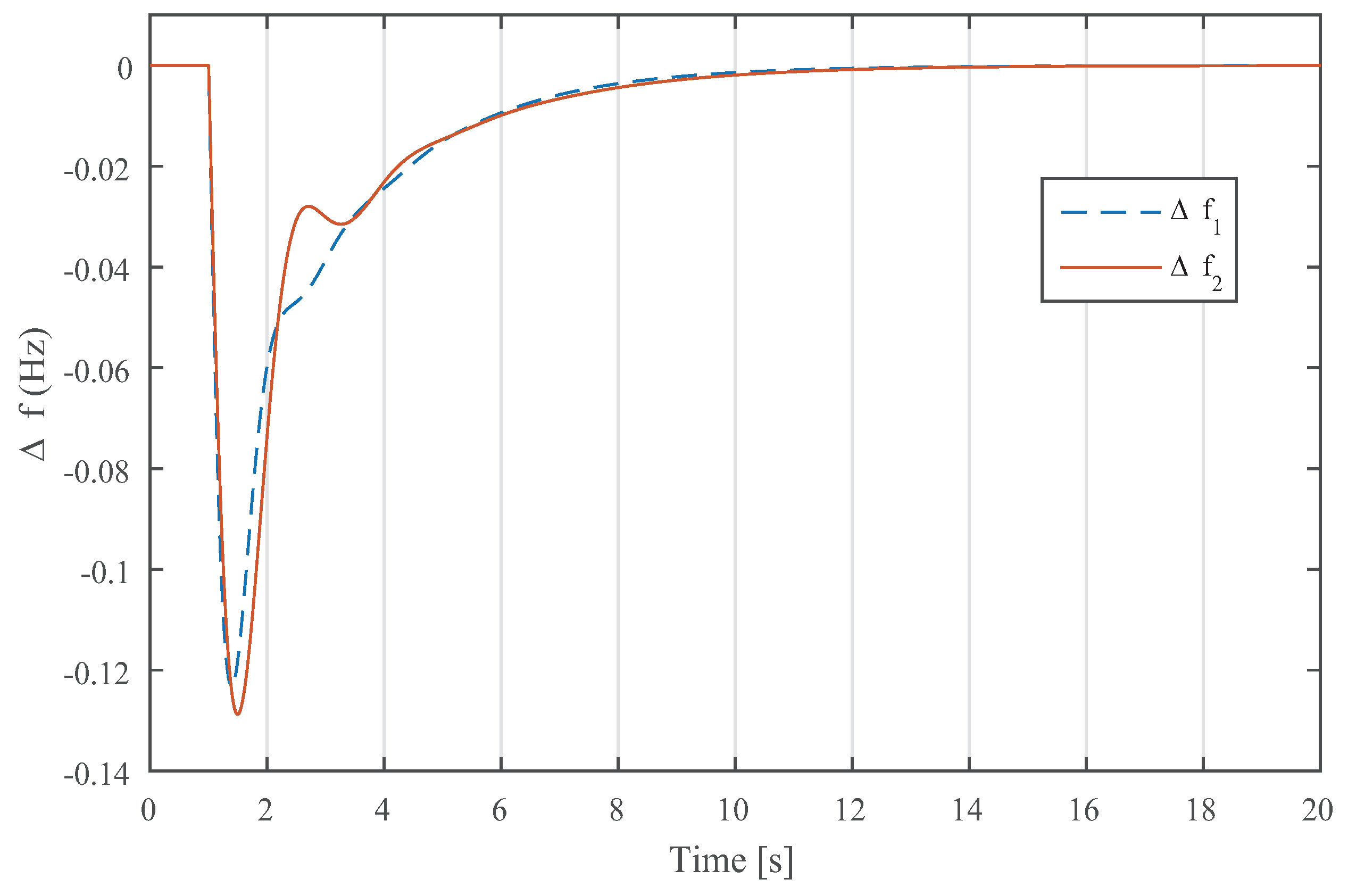
Areas 1 and 2 are identical systems with non-reheated turbines. Firstly, the restriction of SOC is not considered. Then, using the Theorem 2 designs two control laws as follows

$$\begin{array}{c}\hfill \Delta P_{c1}=-1.6886\Delta f_1-1.2560\int \Delta f_{1}dt-0.2879\Delta {\dot{f}}_1\end{array}$$

(29)

and

$$\begin{array}{c}\hfill \Delta P_{c2}=-1.3658\Delta f_2-1.2560\int \Delta f_{2}dt-0.1963\Delta {\dot{f}}_2\end{array}$$

(30)

which show the following results in Figure 3, Figure 4 and Figure 5.

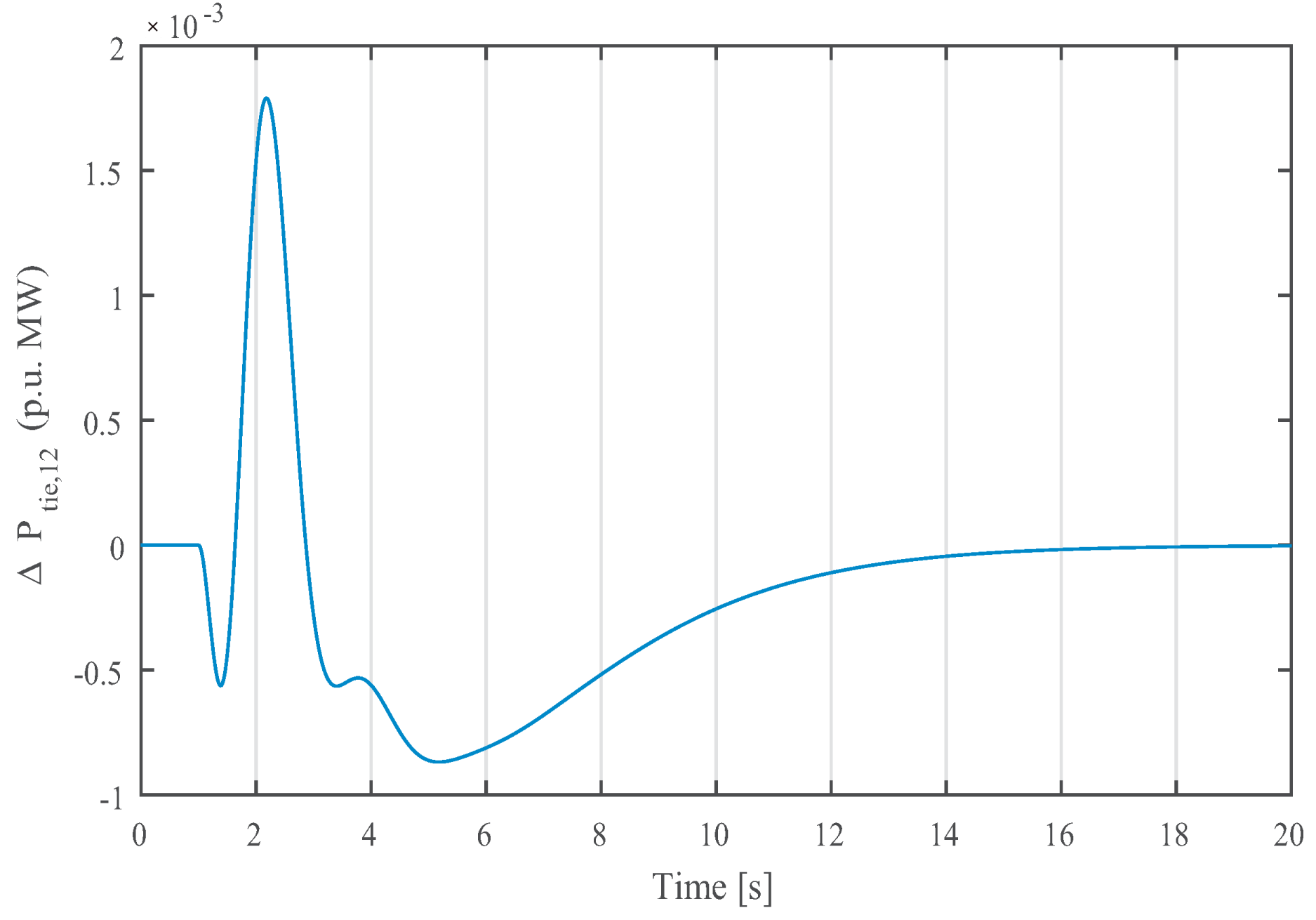
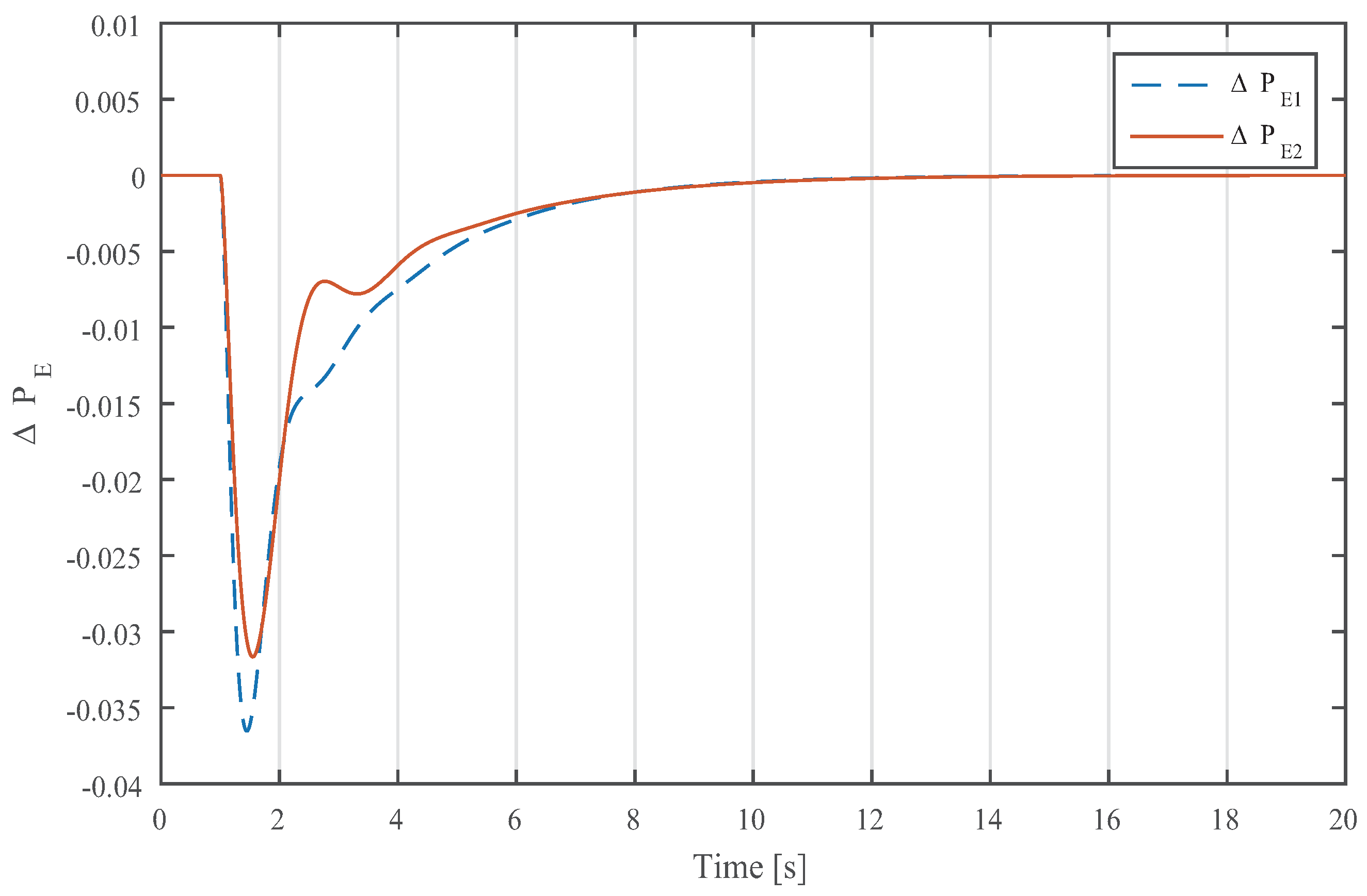
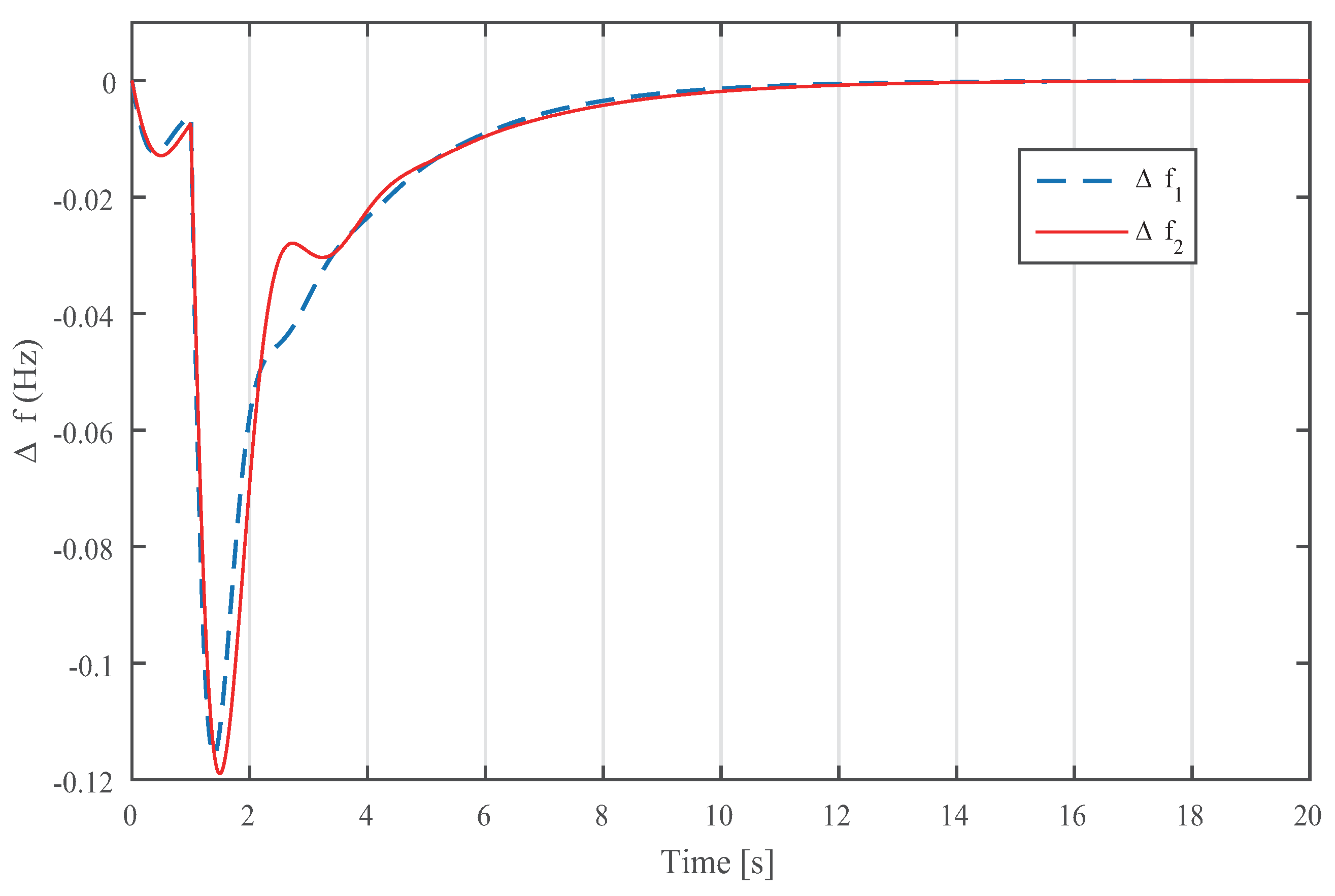
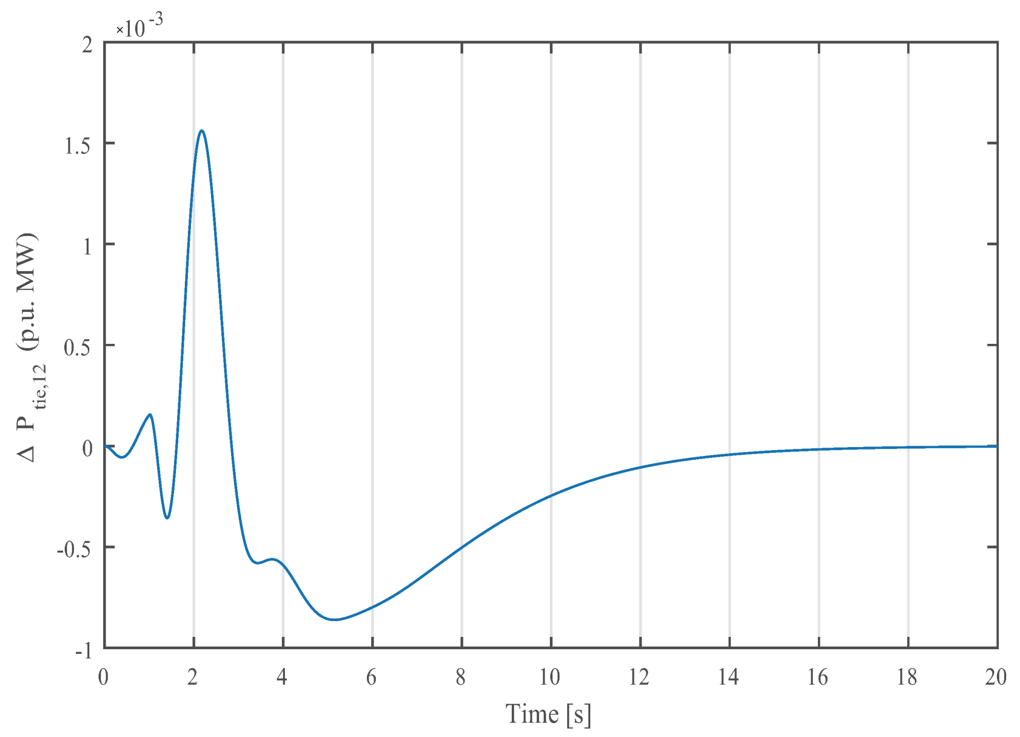
In Figure 3, Figure 4 and Figure 5, when time $t\ge 1$ s, there are the load demands $\Delta P_{L1}=\Delta P_{L2}=0.1$ p.u. MW for the two areas 1 and 2, respectively. Due to the control laws (29) and (30), $\Delta f_1$ and $\Delta f_2$ approach to zero. Based on Equation (5), if $\Delta f_1=\Delta f_2=0$ Hz, there must be $\Delta P_{tie,i}=0$ p.u. MW, which is shown in Figure 4. In the same time, $\Delta P_{E1}$ and $\Delta P_{E2}$ also approach to zero quickly. Thus, the proposed method is effective.

When the above V2G system subjects to SOC, though the plant gain $K_{Ei}$ is still designed by the expression (12), its value must satisfy the region $[0,1]$ decided by the SOC. According to Table 1 and expression (12), the plant gains $K_{E1}$ and $K_{E2}$ are $0.2999$ and $0.2479$, respectively, which obviously belong to the region $[0,1]$. In application, the SOC is usually limited between $[0.2,0.9]$ to keep battery life. Here, the designed values of convert plant gains $K_{E1}$ and $K_{E2}$ also satisfy the region $[0.2,0.9]$. Thus, the above control laws (29) and (30) that are still useful yield the following Figure 6, Figure 7 and Figure 8. When $t>1$ s, there are $\Delta P_{L1}=\Delta P_{L2}=0.1$ p.u. MW for the two areas 1 and 2, respectively. It is clear that the responding curves shown in Figure 6, Figure 7 and Figure 8 prove the validity of Theorem 3.

Since the plant gains $K_{Ei}$ can be computed by the system parameter, it effectively avoids enumerating the values of $K_{Ei}$ from region $[0,1]$ [2,12,13,14,15,16,17]. Moreover, the above control laws (29) and (30) are not only effective for the V2G system is with or without SOC, but also are beneficial for the multi-area LFC system without EVs(the corresponding simulation results by the control laws (29) and (30) are in the paper [7]). The existing methods apply the $H_{\infty }$ control and LMI method to compute the control laws for V2G system and multi-area LFC system without EVs, respectively, while the proposed method reduces the calculated amount of those.

To test the robustness of the proposed method, both of the charging and discharging efficiencies are chosen as $0.92$ [13], and a V2G system containing two areas is simulated for different parameter variations (PV, within $\pm 0.2$). Every area connects with EVs, which batteries subject to SOC and systemic parameters are shown in Table 1. As a result, implementing the control laws (29) and (30) to the mentioned V2G system yields the following Figure 9, Figure 10 and Figure 11. When $t>1$ s, there are $\Delta P_{L1}=\Delta P_{L2}=0.1$ p.u. MW for the two areas 1 and 2, respectively. Then, the responding curves shown in the Figure 9, Figure 10 and Figure 11. imply that the proposed method is robust.

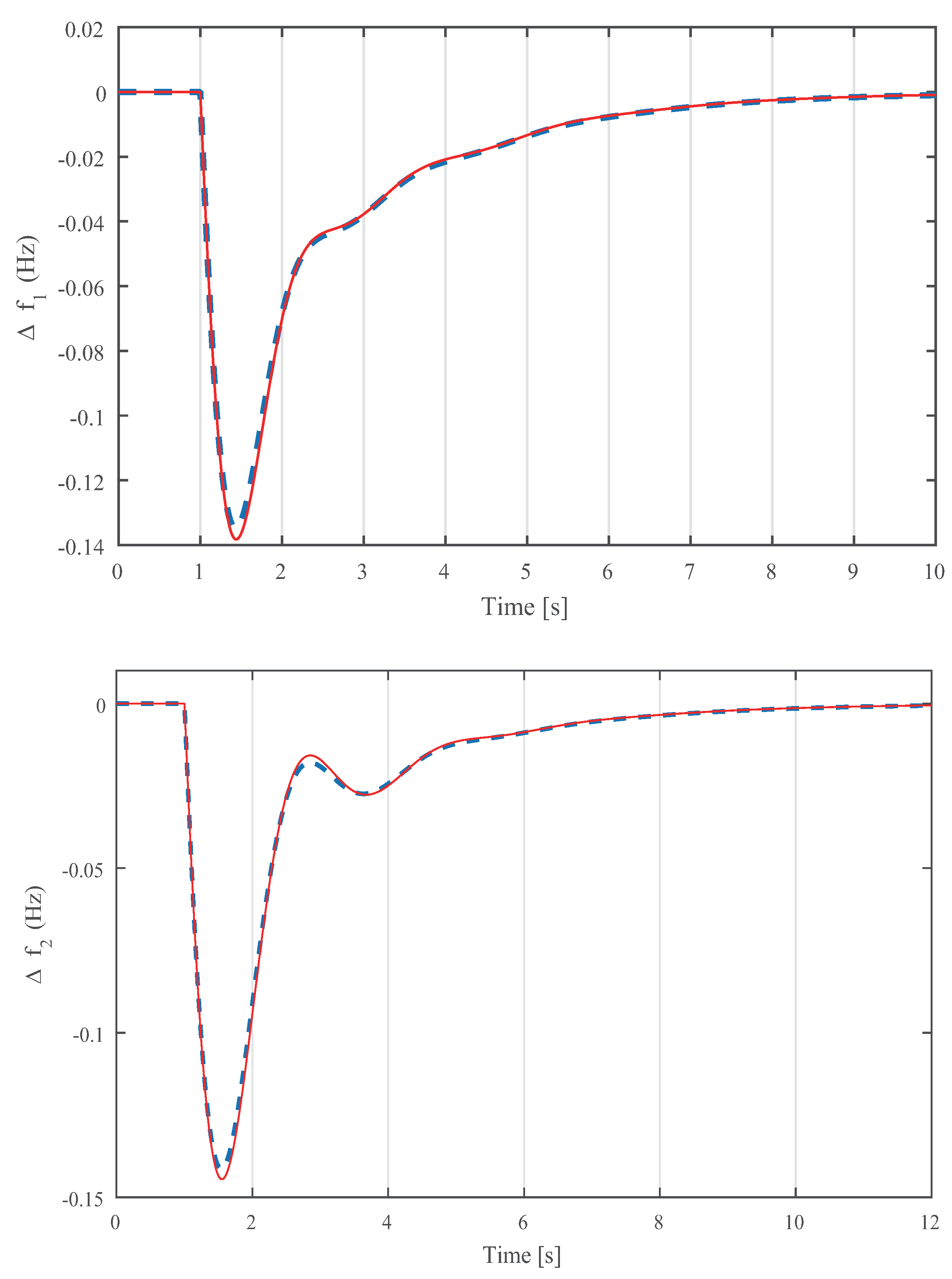
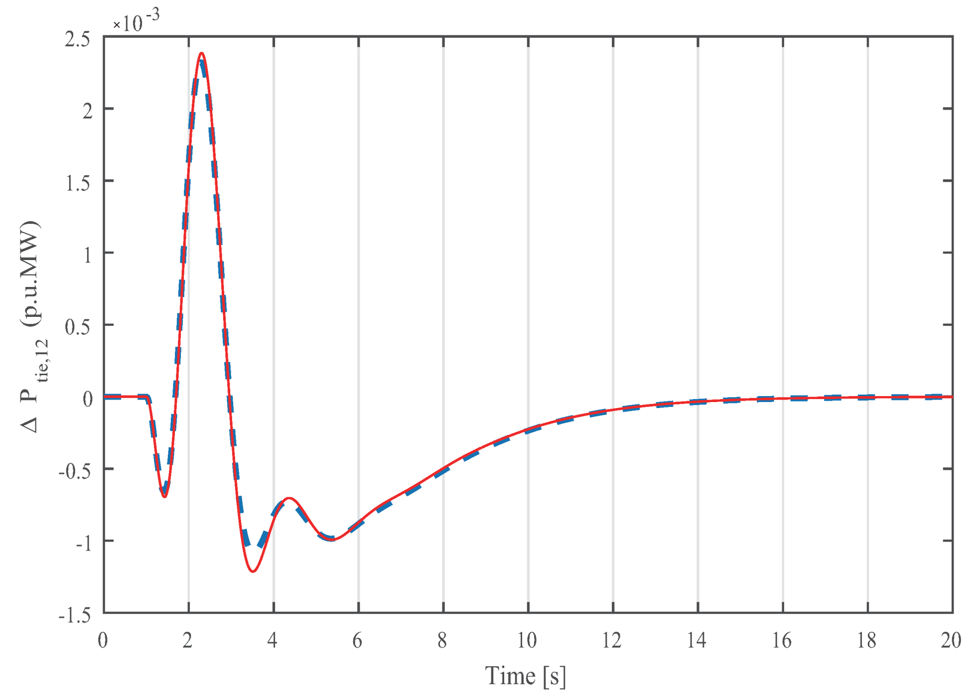
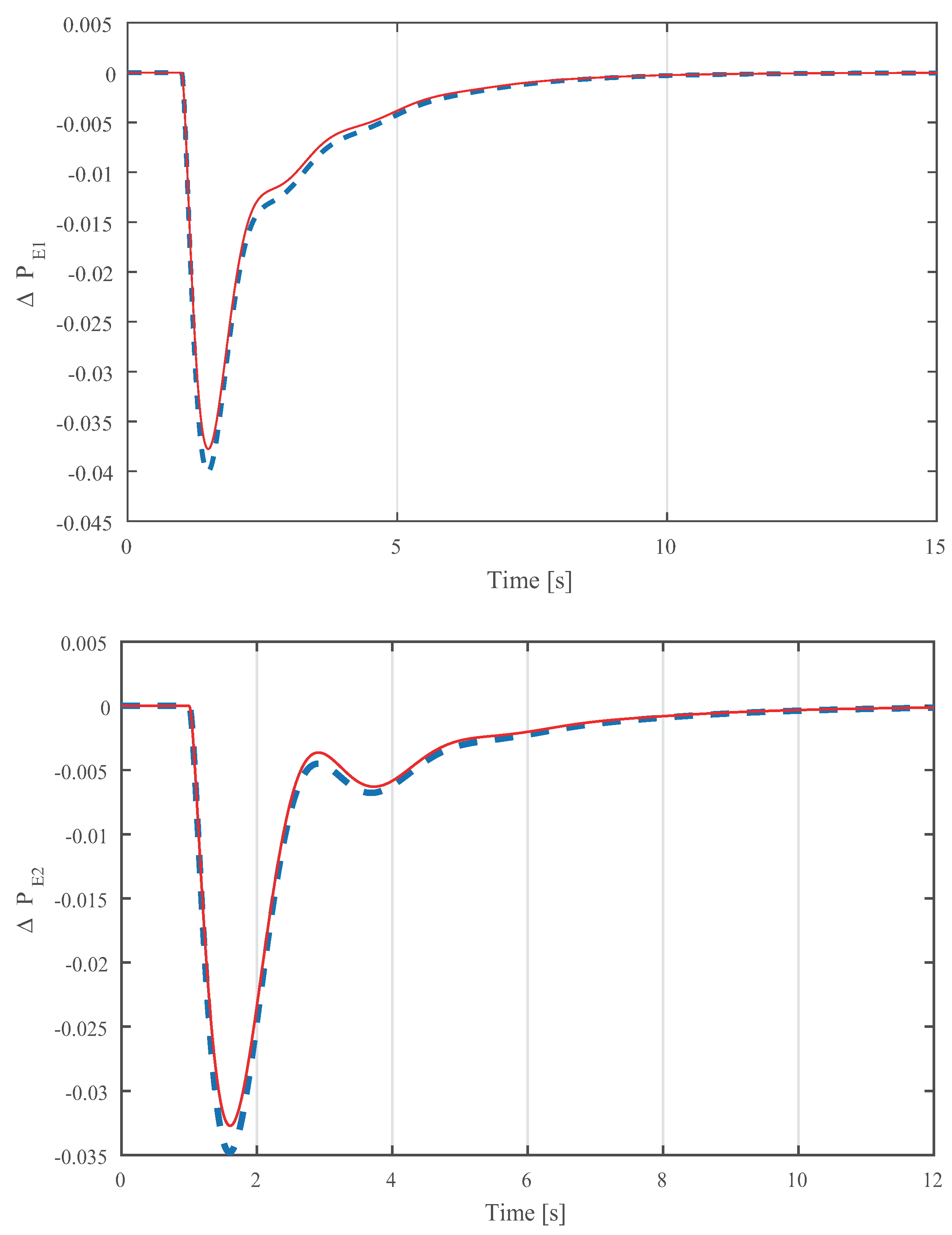
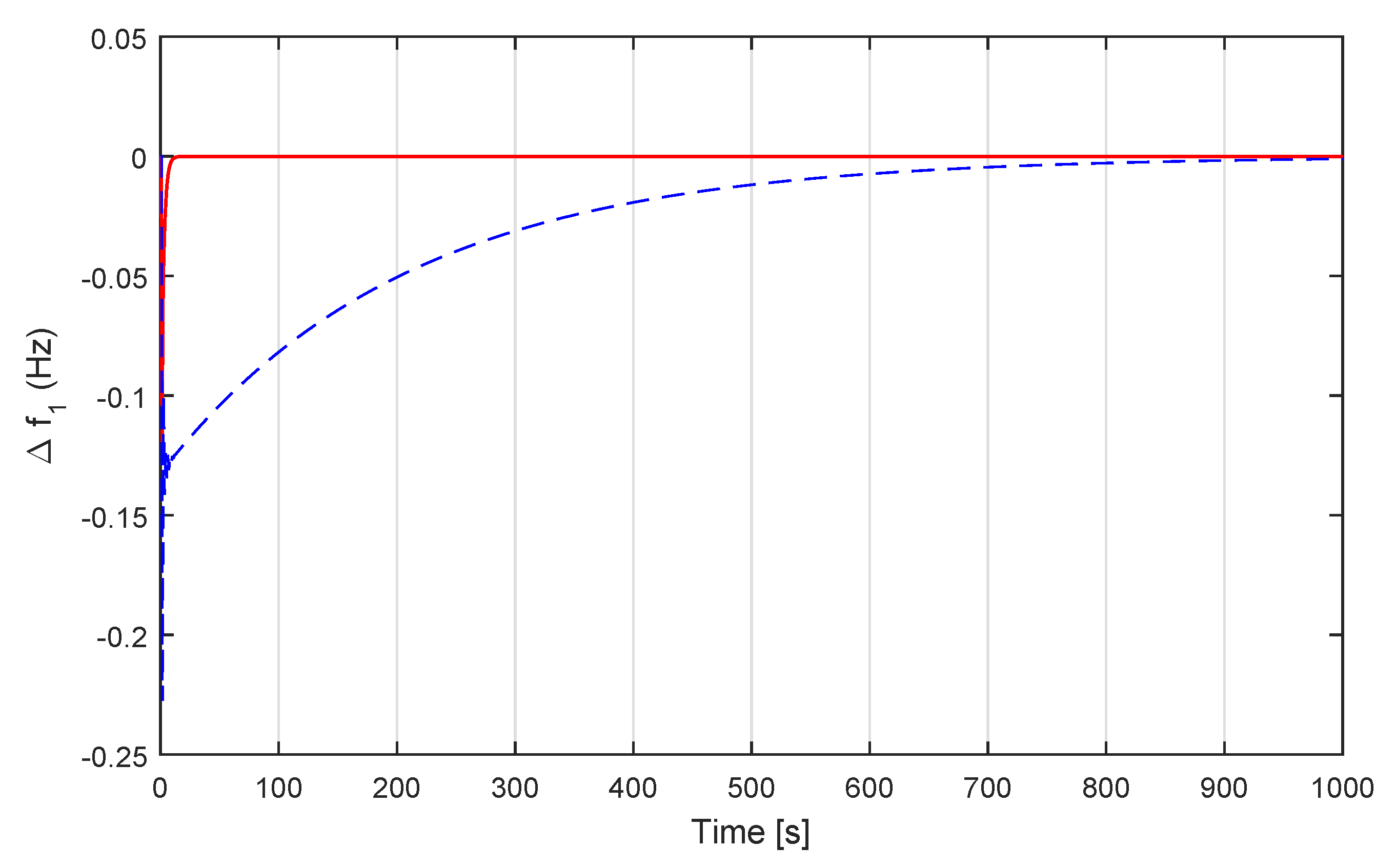
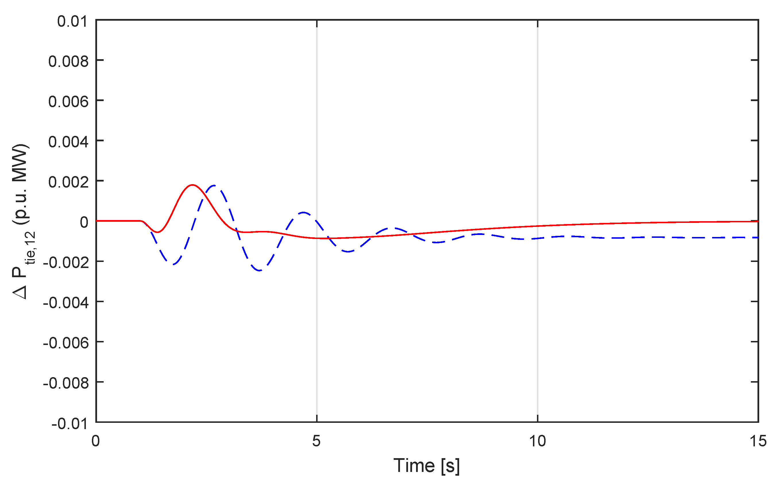
Moreover, due to the parameters of LFC system shown in Table 1 and $\Delta P_{L1}=\Delta P_{L2}=0.1$ p.u. MW for $t>1$, the proposed method is compared with the control law of the paper [10]. Then, the compared results are shown in the following Figure 12, Figure 13 and Figure 14, where the solid lines and dashed lines belong to the proposed method and the control law of paper [10], respectively. It is clear that the convergent speeds of solid lines are faster than the convergent speeds of dashed lines, which implies the advantage of the proposed method.

5. Conclusions

In this paper, two new control methods for the V2G system are proposed with two contributions, i.e., the decouple of the total tie-line power flow $\Delta P_{tie,i}$ and design of the converter plant gain $K_{Ei}$. It is necessary to point out that the converter plant gain are considered as a whole in this paper. In the application, every single converter plant has its value. How to deicide the value of every single converter plant and to research the relationships among the converter plants are still interesting problems.